Resource Allocation for Cost Minimization in Limited Feedback MU-MIMO Systems with Delay Guarantee

Abstract

In this paper, we design a resource allocation framework for the delay-sensitive Multi-User MIMO (MU-MIMO) broadcast system with limited feedback. Considering the scarcity and interrelation of the transmit power and feedback bandwidth, it is imperative to optimize the two resources in a joint and efficient manner while meeting the delay-QoS requirement. Based on the effective bandwidth theory, we first obtain a closed-form expression of average violation probability with respect to a given delay requirement as a function of transmit power and codebook size of feedback channel. By minimizing the total resource cost, we derive an optimal joint resource allocation scheme, which can flexibly adjust the transmit power and feedback bandwidth according to the characteristics of the system. Moreover, through asymptotic analysis, some simple resource allocation schemes are presented. Finally, the theoretical claims are validated by numerical results.

I Introduction

Despite great progress in wireless communications during the past several years, it is still a challenging task to support delay-sensitive wireless services over time-varying fading channels given the scarcity of resources, such as wireless spectrum and energy efficiency. Under these circumstances, efficient resource allocation with delay guarantee (due to its wide applications in video broadcasting or tele-conferencing) becomes a hot topic in wireless research community [1] -[3]. In addition, advanced multiple antennas techniques have became the basic assumption in many international communications standards, e.g. IEEE 802.11ac and LTE-A, in order to support next generation multimedia communications. In particular, Multi-User MIMO (MU-MIMO) is a key technology that has been adopted by IEEE 802.11ac and LTE-A due to its capability to exploit the extra antenna at the base-station to serve multiple users concurrently.

Resource allocation in MU-MIMO systems receives considerable attentions due to its potential of improving spectral efficiency remarkably by exploiting the unique spatial degree of freedom, as seen in [4] -[6] and references therein. As suggested by previous study [7], the performance of MU-MIMO downlink is closely related to the amount of channel state information (CSI) at the base station (BS). For example, if the BS has no CSI, it can only work with a fixed transmission scheme, which is equivalent to the traditional point-to-point MIMO system [8]. If full CSI is available at the BS, dirty paper coding can be used to approach the capacity of MU-MIMO downlink [9]. Between the two extreme cases, if the BS has partial CSI, some effective preprocess techniques, such as zero-forcing beamforming (ZFBF) [10] [11], can be used to partially cancel the inter-user interference. Thus, the amount of CSI greatly impacts the performance of the MU-MIMO system.

Furthermore, the performance of the MU-MIMO system is also affected by other resources, such as transmit power [12], since both the desired signal quality and the inter-user interference are the functions of the transmit power. Note that in the MU-MIMO system, power and feedback resources are interrelated for a given QoS constraint, e.g. delay requirement. For a MU-MIMO system with delay-QoS guarantee, the critical issue of the design of such joint power and feedback resource allocation is to reveal the relationship between the delay requirement and the involved resources. Based on the availability of CSI at the BS, a variety of models have been built to characterize the relationship between the delay requirement and the involved resources, and several adaptive resource allocation schemes have been derived [13], such as equivalent rate constraint [14] [15], Lyapunov drift [16] [17] and Markov decision process (MDP) [18] [19] schemes.

All the aforementioned delay driven resource allocation schemes consider average delay as the QoS requirement. In fact, for some delay sensitive services, e.g. video and audio services, maximum delay is of concern. Based on the large deviation principle, effective bandwidth theory can be used to establish the relationship between maximum delay and minimum serve rate for a given violation probability [20] [21]. Hence [22] studied the power allocation with maximum delay constraint in wireless systems according to the effective bandwidth theory. Nearly all previous works on resource allocation based on the effective bandwidth theory assume full CSI at the BS. However, as mentioned earlier, the BS only has partial CSI by consuming the feedback resource. To the best of our knowledge, feedback resource allocation in the delay-sensitive MU-MIMO downlink has not been well addressed.

In this paper, we focus on joint power and feedback resource allocation with maximum delay guarantee in the MU-MIMO downlink employing with ZFBF. Different from previous works, we consider limited CSI feedback with quantization codebooks. The main contribution of this paper lies in that we reveal the relation between the violation probability with respect to a maximum delay requirement, transmit power and feedback bandwidth based on the effective bandwidth theory, and then derive an optimal joint power and feedback resource allocation scheme by minimizing the resource cost function while satisfying delay constraint. The main contributions of this paper can be summarized as follows:

1. We reveal the relation between the violation probability with respect to a maximum delay requirement, transmit power and feedback bandwidth based on the effective bandwidth theory.

2. We design a framework of joint power and feedback resource allocation in the delay-sensitive downlink MU-MIMO with limited feedback, and propose an optimal joint resource allocation schemes.

3. We formulate a resource cost function as the sum of power cost and feedback cost. By adjusting the relative cost factor according to the characteristics of the considered system, we can obtain the corresponding resource allocation results.

4. Through asymptotic analysis, we obtain two simple resource allocation schemes in the interference-limited and noise-limited scenarios respectively.

The rest of this paper is organized as follows. In Section II, the considered system model is briefly introduced, and then the adopted transmission protocol and effective bandwidth theory are discussed. We propose a joint transmit power and feedback bandwidth allocation scheme with delay-QoS provisioning in Section III. In Section IV, we derive two simple resource allocation schemes via asymptotic analysis. Simulation results are presented in Section V, and we conclude the whole paper in Section VI.

Notation: We use bold upper (lower) letters to denote matrices (column vectors), $(\cdot)^{H}$ to denote conjugate transpose, $(\cdot)^{T}$ to denote matrix transpose, $\|\textbf{x}\|_{2}$ to denote the $l_{2}$ norm of vector x, $|y|$ to denote the absolute value of $y$ and $G^{{}^{\prime}}(x)$ to denote the differential of function $G(x)$ with respect to $x$. The acronym i.i.d. means “independent and identically distributed”, pdf means “probability density function” and cdf means “cumulative distribution function”.

II System Model

Consider a homogeneous MU-MIMO downlink, which includes a base station (BS) with $N_{t}$ antennas, and $N_{t}$ single antenna mobile users (MUs), as shown in Fig.1. For tractability, it is assumed that the downlink channels $\textbf{h}_{k},k=1,\cdots,N_{t}$ from the BS to MUs are i.i.d. complex Gaussian random vectors with zero mean and unit variance. All the channels are assumed to remain unchanged during one time slot and fade independently slot by slot. At the beginning of each time slot, MUs convey the corresponding CSI to the BS based on quantization codebooks. All the codebooks are designed in advance and stored at the BS and MUs. Assuming the codebook of size $2^{B}$ at the $k$th MU is $\mathcal{H}_{k}=\{\hat{\textbf{h}}_{k,1},\cdots,\hat{\textbf{h}}_{k,2^{B}}\},k=1,\cdots,N_{t}$, the optimal quantization codeword selection criterion can be expressed as

$$i=\arg\max\limits_{1\leq j\leq 2^{B}}|\hat{\textbf{h}}_{k,j}^{H}\tilde{\textbf{h}}_{k}|^{2},$$ (1)

where $\tilde{\textbf{h}}_{k}=\frac{\textbf{h}_{k}}{\|\textbf{h}_{k}\|}$ is the channel direction vector. Specifically, the optimal codeword index $i$ is conveyed by the $k$th MU and $\hat{\textbf{h}}_{k,i}$ is recovered at the BS as the instantaneous CSI of the $k$th MU.

Based on the feedback information from the MUs, the BS designs the optimal transmit beams $\textbf{w}_{k},k=1,\cdots,N_{t}$ by making use of the ZFBF design method [10]. For the $k$th MU, the BS first constructs its complementary channel matrix

$${\hat{\textbf{H}}}_{k}=[\hat{\textbf{h}}_{1},\cdots,\hat{\textbf{h}}_{k-1},\hat{\textbf{h}}_{k+1},\cdots,\hat{\textbf{h}}_{N_{t}}],$$

where $\hat{\textbf{h}}_{k-1}$ is the $(k-1)$th MU’s optimal channel quantization codeword. Taking singular value decomposition (SVD) to ${\hat{\textbf{H}}}_{k}$, if $\textbf{V}_{k}^{\perp}$ is the matrix composed of the right singular vectors with respect to zero singular values, then $\textbf{w}_{k}$ is a normalized vector spanned by the space of $\textbf{V}_{k}^{\perp}$, so we have

$$\hat{\textbf{h}}_{u}^{H}\textbf{w}_{k}=0,\quad 1\leq k,u\leq N_{t},u\neq k.$$

It is assumed that $x_{k}$ is the desired normalized signal of the $k$th MU, then its receive signal can be expressed as

$$y_{k}=\sqrt{\frac{P}{N_{t}}}\sum\limits_{u=1}^{N_{t}}\textbf{h}_{k}^{H}\textbf{w}_{u}x_{u}+n_{k},$$ (2)

where $P$ is the total transmit power of the BS, which is equally allocated to the $N_{t}$ MUs. $n_{k}$ is the additive Gaussian white noise with zero mean and variance $\sigma_{n}$ for all MUs. Hence, the ratio of the received signal to interference and noise (SINR) for the $k$th MU can be expressed as

$$\rho_{k} = \frac{P/N_{t}|\textbf{h}_{k}^{H}\textbf{w}_{k}|^{2}}{\sigma_{n}^{2}+P/N_{t}\sum\limits_{u=1,u\neq k}^{N_{t}}|\textbf{h}_{k}^{H}\textbf{w}_{u}|^{2}}$$ (3)

$$= \frac{|\textbf{h}_{k}^{H}\textbf{w}_{k}|^{2}}{1/\gamma+\sum\limits_{u=1,u\neq k}^{N_{t}}|\textbf{h}_{k}^{H}\textbf{w}_{u}|^{2}},$$

where $\gamma=\frac{P}{N_{t}\sigma_{n}^{2}}$ is the average transmit SNR at the BS and $P/N_{t}\sum\limits_{u=1,u\neq k}^{N_{t}}|\textbf{h}_{k}^{H}\textbf{w}_{u}|^{2}$ is the inter-user interference. Although ZFBF is adopted, there are some residual interference, since the BS only has the quantized CSI $\hat{\textbf{h}}_{k},k=1,\cdots,N_{t}$. The beam $\textbf{w}_{u}$ is designed according to the criterion $\hat{\textbf{h}}_{k}^{H}\textbf{w}_{u}=0$, so we have $\textbf{h}_{k}^{H}\textbf{w}_{u}\neq 0$, resulting in the residual interference. Clearly, the more the feedback amount, the less the residual interference. If the BS has full CSI, the interference can be canceled completely due to $\hat{\textbf{h}}_{k}=\tilde{\textbf{h}}_{k}$. It is worth pointing out that the SINRs for all MUs have the similar expression in virtue of the homogeneous characteristics.

II-A Transmission Protocol

The data from high layer is organized in packet at the data link layer. Each packet has a fixed number of bits $N_{b}$, including packet header, payload and cycle redundant check (CRC). The arrived data packets for each MU enter its unique buffer (with infinite capacity) and wait for transmission at the physical layer. Within each transmission duration $T_{b}$, the packets at the front of the buffers are adaptively modulated respectively according to the respective channel quality for the corresponding MU, namely SINR, and then form $N_{t}$ independent data frames. Specifically, the whole SINR range is partitioned into $N$ regions by $N+1$ SINR thresholds $\Omega_{n},n=0,\cdots,N$. For the $k$th MU, if the SINR of the current frame $\rho_{k}$ satisfies the condition that $\Omega_{n}\leq\rho_{k}<\Omega_{n+1}$, then the $n$th modulation format is selected. The determination of SINR threshold depends on the relationship between packet error rate (PER) and modulation mode. Through theoretic analysis and numerical simulation, the expression of PER in the form of modulation mode is given by [24]

$$P_{e,n}(\rho)\approx\left\{\begin{array}[]{ll}1,&\mbox{ if $0<\rho<\gamma_{pn}$}\\ a_{n}\exp(-g_{n}\rho),&\mbox{ if $\rho\geq\gamma_{pn}$}\end{array}\right.$$ (4)

where $\gamma_{pn}$ is the cutoff SINR, below which the PER is unacceptable. Notably, $a_{n}$, $g_{n}$ and $\gamma_{pn}$ are the parameters dependent on the modulation mode $n$. For packet length $N_{b}=1080$, these parameters for various modulation modes can be found in Table I. It is assumed that the objective PER is fixed as $P_{\textrm{obj}}$, a feasible method of determining the $N+1$ SNR thresholds is given by

$$\Omega_{0} = 0,$$

$$\Omega_{n} = \frac{1}{g_{n}}\ln\left(\frac{a_{n}}{P_{\textrm{obj}}}\right),\quad n=1,\cdots,N-1$$

$$\Omega_{N} = \infty.$$ (5)

Due to the delay constraint of real-time services, the packet will be discarded if its waiting time exceeds the upper bound on delay $D_{\textrm{max}}$.

II-B Effective Bandwidth

Since the pioneer work of Kelly [21], the concept of effective bandwidth is widely used in wireless communications together with queueing theory. Effective bandwidth is defined as the characteristics of the source in bounds, limits and approximations for various models of multiplexing under QoS constraints. Specifically, in this paper, effective bandwidth is defined as the minimum serve rate required by a stationary and ergodic arrival process while fulfilling the constraint of maximum waiting delay.

As mentioned earlier, the packet will be discarded if the waiting time is greater than $D_{\textrm{max}}$. Thus, according to the large deviation principle (LDP), the probability of dropping packet caused by delay, so called violation probability, can be written as [23]

$$P_{d}(C)\approx\hat{\rho}\exp\left(-\delta(C)CD_{\textrm{max}}\right),$$ (6)

where $C$ is the serve rate, $\delta(C)=\max(s\geq 0;\alpha(s)\leq C)$ is the QoS exponent, the increasing function $\alpha(s)$ is the so-called effective bandwidth of the traffic source and $s$ denotes the space variable. $\hat{\rho}$ is the probability that the buffer is nonempty. Let $S_{n}$ be the indicator of whether the $n$th packets is in service ($S_{n}\in{0,1}$) and $M$ is the total number of packet, then the approximate nonempty probability $\hat{\rho}$ can be reckoned as

$$\hat{\rho}\approx\frac{1}{M}\sum\limits_{m=1}^{M}S_{m}.$$ (7)

Given the maximum delay constraint $D_{\textrm{max}}$ and the tolerable upper bound on violation probability $\varepsilon=\hat{\rho}\exp\left(-\delta(C)CD_{\textrm{max}}\right)$, we could determine the required minimum serve rate $C_{\textrm{min}}$. For the Poisson arrival process, $\alpha(s)$ can be computed as [21]

$$\alpha(s)=\frac{\lambda}{s}\int_{0}^{\infty}\left(\exp(sx)-1\right)dF(x),$$ (8)

where $F(x)$ is the cumulative distribution function (cdf) of the packet size. Since all packets have the same size, $F(x)$ is a step function at $x=N_{b}$. Thereby, we have

$$\alpha(s)=\frac{\lambda}{s}\left(\exp(sN_{b})-1\right).$$ (9)

By combining (6) and (9), we can obtain the property of the required minimum served rate as follows.

Theorem 1: When the average arrival rate $\lambda$ is large enough, the required minimum served rate can be approximately expressed as $C_{\textrm{min}}(\lambda,D_{\textrm{max}})\simeq N_{b}\lambda-\frac{N_{b}(\ln\varepsilon-\ln\hat{\rho})}{2D_{\textrm{max}}}$. In other words, $C_{\textrm{min}}(\lambda,D_{\textrm{max}})$ increases approximately linearly with $\lambda$.

Proof: Please refer to Appendix I for the proof.

Corollary 1: For high arrival rate, the gap $\Delta_{C}$ between $C_{\lambda,\textrm{min}}(D_{\textrm{max},1})$ and $C_{\textrm{min}}(\lambda,D_{\textrm{max},2})$ is a constant regardless of $\lambda$, where $D_{\textrm{max},1}$ and $D_{\textrm{max},2}$ are two arbitrary maximum delay constraints.

Because $\alpha(s)$ is an increasing function of $s$, $\delta(C)=\max(s\geq 0;\alpha(s)\leq C)$ has a unique solution in the form of $C$. In this context, we could derive the required minimum serve rate $C_{\textrm{min}}(\lambda,D_{\textrm{max}})$ as a function of the QoS requirement $D_{\textrm{max}}$ and $\varepsilon$ for an arbitrary arrival rate $\lambda$ by solving the equations (6) and (9). Similarly, given $C$ and $D_{\textrm{max}}$, we can also obtain the corresponding $\varepsilon$ easily.

III Joint Resource Allocation with Delay Guarantee

In this section, we focus on joint transmit power and feedback bandwidth allocation while satisfying the delay constraint in a MU-MIMO downlink. Note that in this paper transmit power is the same for all MUs and only the total power is regulated, since equal power allocation is optimal in the statistical sense and can avoid a large amount of information feedback in a multiuser system. Considering the scarcity of the two resources in practical systems, we expect to minimize the total resource utilization. Hence, we set the optimization objective as minimizing the following resource cost function:

$$\eta=\varphi P+\psi N_{t}B,$$ (10)

where $\varphi$ (cost per watt) and $\psi$ (cost per bit) are the cost factors of transmit power $P$ and feedback amount $N_{t}B$, respectively. The cost factors depends on the characteristics of the considered system. For example, in a power-limited system, more feedback amount should be used to decrease the consumption of transmit power. Otherwise, if the system is feedback limited, it is better to use more transmit power. By changing the relative cost factor $\xi=\frac{\varphi}{\psi}$, we can character the different systems. As a simple example, $\xi>>1$ denotes the power-limited system, while $\xi<<1$ denotes the feedback-limited system. Since the two resources are independent of each other, we model the total cost as the linear sum of the two resource costs.

As analyzed earlier, given data arrival rate, the violate probability with respect to a maximum delay constraint is a function of the serve rate. Thus, based on adaptive modulation, the average violation probability for the $k$th MU with transmit power $P$ and codebook size $B$ can be computed as

$$\bar{\varepsilon}_{k}(P,B) = \sum\limits_{n=0}^{N}P_{d}(C_{n})P_{r}(C_{n})$$ (11)

$$= \sum\limits_{n=0}^{N}P_{d}(C_{n})\bigg{(}F_{\rho_{k}}(\Omega_{n+1})-F_{\rho_{k}}(\Omega_{n})\bigg{)},$$

where $F_{\rho_{k}}(x)$ is the cumulative distribution function (cdf) of SINR $\rho_{k}$, and $P_{r}(C_{n})=F_{\rho_{k}}(\Omega_{n+1})-F_{\rho_{k}}(\Omega_{n})$ is the probability that the $n$th serve rate or modulation mode is selected. Assuming the downlink bandwidth is $W$, then we have $C_{n}=nW/N_{b}$. For the $n$th modulation mode or given the serve rate $C_{n}$, the nonempty probability $\rho(C_{n})$ and the QoS exponent $\delta(C_{n})$ are fixed based on (6) and (9), so the violation probability $P_{d}(C_{n})$ is a constant. Following [10] [11], the cdf of $\rho_{k}$ based on limited feedback ZFBF can be expressed as

$$F_{\rho_{k}}(x)=1-\frac{\exp\left(-x/\gamma\right)}{\left(1+\theta x\right)^{N_{t}-1}},$$ (12)

where $\theta=2^{-\frac{B}{N_{t}-1}}$. Substituting (12) into (11), we have

$$\bar{\varepsilon}_{k}(P,B) = \sum\limits_{n=0}^{N}P_{d}(C_{n})\left(\frac{\exp\left(-\Omega_{n}/\gamma\right)}{\left(1+\theta\Omega_{n}\right)^{N_{t}-1}}-\frac{\exp\left(-\Omega_{n+1}/\gamma\right)}{\left(1+\theta\Omega_{n+1}\right)^{N_{t}-1}}\right)$$ (13)

$$= P_{d}(C_{0})-\sum\limits_{n=1}^{N}\bigg{(}P_{d}(C_{n-1})-P_{d}(C_{n})\bigg{)}\frac{\exp\left(-\Omega_{n}/\gamma\right)}{\left(1+\theta\Omega_{n}\right)^{N_{t}-1}}.$$

Therefore, cost-minimizing joint resource allocation with delay guarantee is equivalent to the following optimization problem

$$J_{1}:\min\limits_{P,B} \eta=\varphi P+\psi N_{t}B$$ (14)

$$s.t.\quad \bar{\varepsilon}_{k}(P,B)\leq\varepsilon_{0},k=1,\cdots,N_{t}$$

$$P\leq P_{0}$$

$$B\leq B_{0},$$

where $\varepsilon_{0}$, $P_{0}$ and $B_{0}$ are the constraints on violation probability, transmit power and feedback bandwidth, respectively. Since $B$ is an integer variable, $J_{1}$ is a mixed integer programming problem, it is difficult to obtain a closed-form expression for the optimal $P$ and $B$. Intuitively, the optimal algorithm is to compute the transmit power by letting $\bar{\varepsilon}_{k}(P,B)=\varepsilon_{0}$ for a given $B$. Then, search the optimal resource combination with the minimum resource cost by scaling $B$ from 1 to $B_{0}$, namely the exhaustive search algorithm. In fact, $J_{1}$ can be transformed as a general optimization problem if $B$ is relaxed to a nonnegative real variable, so that it can be solved by some optimization softwares, such as the Lingo. Assuming $P^{{\dagger}}$ and $B^{{\dagger}}$ are the optimal solutions of the relaxed optimization problem, where $B^{{\dagger}}$ may not be an integer. Under this condition, we take $B_{c}=\lceil B^{{\dagger}}\rceil$ and $B_{f}=\lfloor B^{{\dagger}}\rfloor$ as the two candidates, where $\lceil B^{{\dagger}}\rceil$ and $\lfloor B^{{\dagger}}\rfloor$ mean the smallest integer not less than $B^{{\dagger}}$ and the largest integer not greater than $B^{{\dagger}}$, respectively. Given $B_{c}$, we could get the optimal transmit power $P_{c}$ by letting $\bar{\varepsilon}_{k}(P_{c},B_{c})=\varepsilon_{0}$ and the corresponding resource cost function $\eta(P_{c},B_{c})$. Similarly, we also could obtain $P_{f}$ and $\eta(P_{f},B_{f})$ based on $B_{f}$. Then, if $\eta(P_{c},B_{c})<\eta(P_{f},B_{f})$, we take $(P_{c},B_{c})$ as the final resource combination. Otherwise, $(P_{f},B_{f})$ is selected. Thus, we proposed a joint resource allocation scheme based on the above idea. First, we derive the optimal feedback amount and transmit power based on the relaxed optimization problem by using the Lingo. Then, we round the feedback amount to two nearest integers, and compute the maximum transmit power while fulfilling delay constraint. Finally, by comparing the corresponding resource cost, the resource combination with the smallest cost is selected. The joint resource allocation scheme can be described as follows  

1. Initialization: given $N_{t}$, $N$, $P_{0}$, $B_{0}$, $\varphi$ and $\psi$.

2. Relax $B$ to a nonnegative real number and derive $P^{{\dagger}}$ and $B^{{\dagger}}$ by the Lingo.

3. Let $B_{c}=\lceil B^{{\dagger}}\rceil$ and $B_{f}=\lfloor B^{{\dagger}}\rfloor$. Compute $P_{c}$ satisfying $\bar{\varepsilon}_{k}(P_{c},B_{c})=\varepsilon_{0}$ and $P_{f}$ satisfying $\bar{\varepsilon}_{k}(P_{f},B_{f})=\varepsilon_{0}$.

4. Let $\eta(P_{c},B_{c})=\varphi P_{c}+\psi N_{t}B_{c}$ and $\eta(P_{f},B_{f})=\varphi P_{f}+\psi N_{t}B_{f}$. If $\eta(P_{c},B_{c})<\eta(P_{f},B_{f})$, $(P_{c},B_{c})$ is the final resource combination. Otherwise, $(P_{f},B_{f})$ is the required one.

 

Interestingly, it is found that although the proposed algorithm is derived based on the relaxed optimization problem, it is also optimal together with the exhaustive search algorithm. The complete proof is given by Appendix II.

IV Asymptotical Analysis

In this section, we analyze the asymptotical characteristics of violation probability in some special cases. Based on the insight from the analysis, we can then derive some simple resource allocation schemes that are optimal asymptotically.

IV-A Interference-Limited Case

If the variance of noise is quite small, e.g. in the noise-free scenario, the noise can be negligible with respect to the inter-user interference, namely the interference-limited case. Under such a condition, the received SINR of the $k$th MU can be approximated as

$$\rho_{k}\approx\frac{|\textbf{h}_{k}^{H}\textbf{w}_{k}|^{2}}{\sum\limits_{u=1,u\neq k}^{N_{t}}|\textbf{h}_{k}^{H}\textbf{w}_{u}|^{2}}.$$ (15)

According to the analysis in previous section, we have the cdf of $\rho_{k}$ in this case as

$$F_{\rho_{k}}(x)=1-(1+\delta x)^{-(N_{t}-1)}.$$ (16)

Thereby, the joint resource allocation can be described as the following optimization problem

$$J_{2}:\min\limits_{P,B} \eta=\varphi P+\psi N_{t}B$$ (17)

$$s.t.\quad P_{d}(C_{0})-\sum\limits_{n=1}^{N-1}\bigg{(}P_{d}(C_{n-1})-P_{d}(C_{n})\bigg{)}\left(1+\Omega_{n}2^{-\frac{B}{N_{t}-1}}\right)^{-(N_{t}-1)}\leq\varepsilon_{0}$$

$$P\leq P_{0}$$

$$B\leq B_{0}.$$

It is found that the first constraint is independent of $P$, this is because the effects of $P$ on the desired signal and interference are canceled out each other when the noise is ignored. From the perspective of the optimization, it seems that $P=0$ is the optimal solution to $J_{2}$. However, in practical systems, a minimum transmit power is required to maintain the communications. In other words, $P$ is set as the required minimum transmit power. For the optimal codebook size, we first compute the $B^{{\dagger}}$ satisfying $P_{d}(C_{0})-\sum\limits_{n=1}^{N-1}\bigg{(}P_{d}(C_{n-1})-P_{d}(C_{n})\bigg{)}\left(1+\Omega_{n}2^{-\frac{B}{N_{t}-1}}\right)^{-(N_{t}-1)}=\varepsilon_{0}$ and then let $B=\lceil B^{{\dagger}}\rceil$ because of its integer constraint.

IV-B Noise-Limited Case

If the noise is quite large, the inter-user interference can be negligible compared with the noise, namely the noise-limited case. In this scenario, the received SINR of the $k$th MU can be approximated as

$$\rho_{k}\approx\gamma|\textbf{h}_{k}^{H}\textbf{w}_{k}|^{2}.$$ (18)

Similarly, we have the cdf of $\rho_{k}$ in this case as

$$F_{\rho_{k}}(x)=1-\exp\bigg{(}\frac{x}{\gamma}\bigg{)}.$$ (19)

Hence, we could formulate the joint resource allocation as the following optimization problem

$$J_{3}:\min\limits_{P,B} \eta=\varphi P+\psi N_{t}B$$ (20)

$$s.t.\quad P_{d}(C_{0})-\sum\limits_{n=1}^{N-1}\bigg{(}P_{d}(C_{n-1})-P_{d}(C_{n})\bigg{)}\exp\left(-\Omega_{n}N_{t}\sigma_{n}^{2}/P\right)\leq\varepsilon_{0}$$

$$P\leq P_{0}$$

$$B\leq B_{0}.$$

In this case, $B=0$ is the optimal solution to $J_{3}$, which is consistent with our intuition. This is because when the noise is dominant, CSI feedback hardly affects the SINR. Furthermore, the optimal $P$ can be obtained by solving the function $P_{d}(C_{0})-\sum\limits_{n=1}^{N-1}\bigg{(}P_{d}(C_{n-1})-P_{d}(C_{n})\bigg{)}\exp\left(-\Omega_{n}N_{t}\sigma_{n}^{2}/P\right)=\varepsilon_{0}$.

V Performance Analysis and Simulation Results

To examine the effectiveness of the proposed cost minimizing joint transmit power and feedback bandwidth allocation scheme with delay guarantee, we present several numerical results in different scenarios. For all scenarios, we set $N_{t}=4$, $N=8$, $W=1$MHz, $\sigma_{n}^{2}=1$, $P_{\textrm{obj}}=10^{-4}$ and $N_{b}=1080$ for convenience. Noticeably, considering resource limitation, we set $P_{0}=40$dB and $B_{0}=10$. The codebooks are designed based on vector quantization (VQ) method [25] [26].

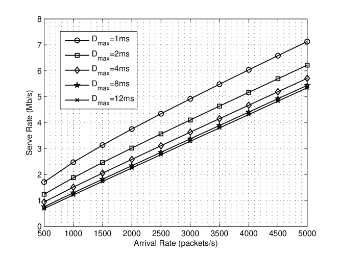
Figure 2: Minimum required served rate for high arrival rate.

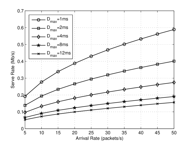
Figure 3: Minimum required served rate for low arrival rate.

Fig.2 and Fig.3 show the required minimum served rates $C_{\textrm{min}}(\lambda,D_{\textrm{max}})$ for the scenarios with high and low arrival rates respectively when $\varepsilon_{0}=0.01$. Depending on the arrival rates, we can see that there are different trends for the served rates in these two scenarios. For high arrival rate $\lambda$, minimum serve rate increases approximately linearly, which is well consistent with Theorem 1. However, for low arrival rate, the maximum delay constraint $D_{\textrm{max}}$ has a great impact on the slope of variation of the required serve rate, where the slope is inversely proportional to $D_{\textrm{max}}$. As seen in Fig.3, when $D_{\textrm{max}}$ is greater than $8$ms, the slope is approaching zero asymptotically. In addition, the gap of the required serve rates $\Delta_{C}=C_{\textrm{min}}(D_{\textrm{max},1})-C_{\textrm{min}}(D_{\textrm{max},2})$ is not a linear function of $\Delta_{D}=D_{\textrm{max},1}-D_{\textrm{max},2}$. For example, the gap of the required serve rates due to the delay relaxation from $D_{\textrm{max}}=8$ms to $4$ms is larger than the delay relaxation from $D_{\textrm{max}}=12$ms to $8$ms.

In Tab.II, we compare the joint resource allocation results based on the proposed algorithm and exhaustive search algorithm. For ease of comparison, we fix arrival rate as $\lambda=300$ packets/s and the upper bound on average violation probability $\varepsilon_{0}=0.01$. In addition, we use $\xi=\psi/\varphi$ to denote the relative cost factor. For a strict delay constraint, such as $D_{\textrm{max}}=2$ms, with the increase of the relative cost factor, the optimal feedback bandwidth decreases accordingly while the required transmit power increases, this is because as the cost factor of feedback bandwidth increases, higher transmit power has a lower total cost while satisfying the delay constraint. Therefore, we could flexibly adjust the resource combination by changing the relative cost factor according to the characteristics of the considered system. Moreover, it is found that the proposed algorithm gets the same results as exhaustive search algorith, which reconfirms our theoretical claim. For the case with loose constraint, e.g. $D_{\textrm{max}}=8$ms, the above observations also hold true. Comparing with the allocation results with the same $\xi$, the two cases use the same feedback bandwidth, but the case with $D_{\textrm{max}}=2$ms has a higher transmit power, since it is relatively cheaper to add more power than to reduce feedback bandwidth.

VI Conclusion

A major contribution of this paper is to provide a framework of joint transmit power and feedback bandwidth allocation with delay guarantee so that the two scarce resources can be utilized in a more efficient manner according to the characteristics of a multi-user MIMO broadcast system. First, according to the effective bandwidth theory, we established the intrinsic relationship between minimum required serve rate and maximum delay constraint. Then, based on adaptive modulation, we formulated the average violation probability with respect to maximum delay in terms of transmit power and codebook size. Eventually, by minimizing the total resource cost while satisfying the delay constraint, an optimal joint resource allocation scheme was derived accordingly.

Appendix A Proof of Theorem 1

Given $N_{b}$, $D_{\textrm{max}}$ and $\varepsilon$, if the arrival rate is large enough, in order to ensure that $\varepsilon$ is a positive constant between 0 and 1, $s=\delta(C)$ should be a positive constant close to zero. Thereby, $\exp(sN_{b})$ in (9) can be approximately expressed as $1+N_{b}s+N_{b}^{2}s^{2}$ by Taylor expansion at the point zero so that $C_{\textrm{min}}(D_{\textrm{max}})=\alpha(s)\simeq\lambda(N_{b}+N_{b}^{2}s/2)$ by substituting $\exp(sN_{b})\simeq 1+N_{b}s+N_{b}^{2}s^{2}/2$ into (9). Meanwhile, by replacing $C$ in (6) with $\lambda(N_{b}+N_{b}^{2}s/2)$, we have

$$\varepsilon\simeq\hat{\rho}\exp(-\lambda N_{b}D_{\textrm{max}}(1+sN_{b}/2)s).$$ (21)

Rearranging (21), it is obtained that

$$\frac{N_{b}}{2}s^{2}+s+\frac{a(\lambda,D_{\textrm{max}})}{N_{b}}=0,$$ (22)

where $a(\lambda,D_{\textrm{max}})=\frac{\ln\varepsilon-\ln\hat{\rho}}{\lambda D_{\textrm{max}}}$. By solving the function (22), we have

$$s=\frac{\sqrt{1-2a(\lambda,D_{\textrm{max}})}-1}{N_{b}}.$$ (23)

Therefore, the required minimum served rate can be approximately expressed as

$$C_{\textrm{min}}(D_{\textrm{max}}) \simeq \lambda(N_{b}+N_{b}^{2}s/2)$$ (24)

$$= \frac{N_{b}}{2}\lambda+\frac{N_{b}}{2}\lambda\sqrt{1-2a(\lambda,D_{\textrm{max}})}$$

$$\approx N_{b}\lambda-\frac{N_{b}(\ln\varepsilon-\ln\hat{\rho})}{2D_{\textrm{max}}},$$

where (24) follows from the fact that $\sqrt{1+x}\approx 1+\frac{x}{2}$, if $-1<x\leq 1$. Thereby, we validate the claim of Theorem 1.

Appendix B Proof of the optimality of joint resource allocation scheme

Assume $\cup(P_{i},B_{i})$, $i=0,1,\cdots,B_{0}$, where $B_{i}=i$, is the set of all the feasible solutions of $J_{1}$. If $B^{\dagger}$ is an integer, then $(P^{\dagger},B^{\dagger})$ is also the optimal solution of $J_{1}$ definitely. Otherwise, we take $B_{c}=\lceil B^{\dagger}\rceil$ and $B_{f}=\lfloor B^{\dagger}\rfloor$ as the two candidates, and derive the corresponding optimal transmit power $P_{c}$ and $P_{f}$. Since the violation probability is the monotonously decreasing function of $P$ and $B$, we have $P_{c}<P_{f}$. In what follows, we prove $(P_{c},B_{c})$ is the optimal solution of $J_{1}$ if $\eta(P_{c},B_{c})<\eta(P_{f},B_{f})$, otherwise $(P_{f},B_{f})$ is the optimal solution. Prior to the proof, we first present the following lemma:

Lemma 1: Given the requirement of the violation probability, the reduction of transmit power $\triangle P$ becomes smaller gradually by adding the same feedback bandwidth $\triangle B$ as feedback bandwidth $B$ increases.

Lemma 1 holds true since the violation probability is a power function of feedback bandwidth. If $\eta(P_{c},B_{c})<\eta(P_{f},B_{f})$, then the cost of the added 1bit feedback bandwidth is less than that of the reduced transmit power. Assuming $(P_{f-1},B_{f-1})$ is the feasible solution of $J_{1}$, due to $P_{f-1}-P_{f}>P_{f}-P_{c}$ according to Lemma 1, we have $\eta(P_{f-1},B_{f-1})>\eta(P_{f},B_{f})$. Thus, it is obtained that $\eta(P_{i},B_{i})>\eta(P_{f},B_{f})>\eta(P_{c},B_{c})$ for all $i<f$. We consider the case of $i>c$. Assuming $\eta(P_{i},B_{i})<\eta(P_{c},B_{c})$ and $(P^{{}^{\prime}},B^{{}^{\prime}})$ is a feasible solution of the relaxed problem, where $B^{{}^{\prime}}-B^{\dagger}=B_{i}-B_{c}$. According to Lemma 1, we have $P^{\dagger}-P^{{}^{\prime}}>P_{c}-P_{i}$ because of $B^{\dagger}<B_{c}$. If $\eta(P_{i},B_{i})<\eta(P_{c},B_{c})$, we have $\eta(P^{{}^{\prime}},B^{{}^{\prime}})<\eta(P^{\dagger},B^{\dagger})$. However, $(P^{\dagger},B^{\dagger})$ is the optimal solution of the relaxed problem, it is impossible to find the $(P^{{}^{\prime}},B^{{}^{\prime}})$ such that $\eta(P^{{}^{\prime}},B^{{}^{\prime}})<\eta(P^{\dagger},B^{\dagger})$. In other words, $\eta(P_{i},B_{i})<\eta(P_{c},B_{c})$ for any $i>c$ can not hold true. Hence, $(P_{c},B_{c})$ is the optimal solution of $J_{1}$. Similarly, if $\eta(P_{c},B_{c})>\eta(P_{f},B_{f})$, $(P_{f},B_{f})$ is optimal.

Figure 1: The considered system block diagram.

TABLE I: The Important Parameters for Different Modulation Modes

	Mode 1	Mode 2	Mode 3	Mode 4	Mode 5	Mode 6	Mode 7
Modulation	BPSK	QPSK	8QAM	16QAM	32QAM	64QAM	128QAM
Rate (bits/sym.)	1	2	3	4	5	6	7
$a_{n}$	67.7328	73.8279	58.7332	55.9137	50.0552	42.5594	40.2559
$g_{n}$	0.9819	0.4945	0.1641	0.0989	0.0381	0.0235	0.0094
$\gamma_{pn}(dB)$	6.3281	9.3945	13.9470	16.0938	20.1103	22.0340	25.9677

TABLE II: Resource Allocation Results for Different Relative Cost Factor

		$\xi$	80	120	160	200	240
		$B$	10	8	7	6	5
$D_{\textrm{max}}=2$ms	Exhaustive Search Algorithm	$P$(dB)	38.0	38.6	38.9	39.3	39.8
		$B$	10	8	7	6	5
	Proposed Algorithm	$P$(dB)	38.0	38.6	38.9	39.3	39.8
		$B$	10	8	7	6	5
$D_{\textrm{max}}=8$ms	Exhaustive Search Algorithm	$P$(dB)	37.7	38.2	38.6	39.0	39.4
		$B$	10	8	7	6	5
	Proposed Algorithm	$P$(dB)	37.7	38.2	38.6	39.0	39.4

References

- [1] J. Miao, Z. Hu, K. Yang, C. Wang, and H. Tian, “Joint power and bandwidth allocation algorithm with QoS support in heterogeneous wireless networks,” IEEE Commun. Lett., vol. 16, no. 4, pp. 479-481, Apr. 2012.
- [2] D. Zhang, M. Tao, J. Lu, and M. Wang, “Dynamic resource allocation for real-time service in cooperative OFDMA systems,” IEEE Commun. Lett., vol. 15, no. 5, pp. 479-499, May 2011.
- [3] N. U. Hassan, and M. Assaad, “Dynamic resource allocation in multi-service OFDMA systems with dynamic queue control,” IEEE Trans. Commun., vol. 59, no. 6, pp. 1664-1674, Jun. 2011.
- [4] Y. Cui, Q. Huang, and V. K. N. Lau, “Queue-aware dynamic clustering and power allocation for network MIMO systems via distributed stochastic learning,” IEEE Trans. Signal Process., vol. 59, no. 3, pp. 1229-1239, Mar. 2011.
- [5] O. Souihli, and T. Ohtsuki, “Joint feedback and scheduling scheme for service-differentiated multiuser MIMO systems,” IEEE Trans. Wireless Commun., vol. 9. no. 2, pp. 528-533, Feb. 2010.
- [6] X. Chen, Z. Zhang, S. Chen, and C. Wang, ”Adaptive mode selection for multiuser MIMO downlink employing rateless codes with QoS provisioning,” IEEE Trans. Wireless Commun., vol. 11, no. 2, pp. 790-799, Feb. 2012.
- [7] B. Hassibi, and M. Sharif, “Fundamental limits in MIMO broadcast channels,” IEEE Journal on Sel. Areas in Commun., vol. 25, no. 7, pp. 1333-1344, Sep. 2007.
- [8] M. Sharif, and B. Hassibi, “On the capacity of MIMO broadcast channels with partial side information,” IEEE Trans. Inf. Theory, vol. 51, no. 2, pp. 506-522, Feb. 2005.
- [9] G. Caire, and S. Shamai, “On the achievable throughput of a multiantenna gaussian broadcast channel,” IEEE Trans. Inf. Theory, vol. 49, no. 7, pp. 1691-1706, Jul. 2003.
- [10] X. Chen, and C. Yuen, “Efficient resource allocation in rateless coded MU-MIMO cognitive radio network with QoS provisioning and limited feedback,” IEEE Trans. Veh. Tech., vol. 62, no. 1, pp. 395-399, Jan. 2013.
- [11] J. Zhang, M. Kountouris, J. G. Andrews, and R. W. Heath, Jr., “Multi-mode transmission for the MIMO broadcast channel with imperfect channel state information,” IEEE Trans. Commun., vol. 59, no. 3, pp. 803-814, Mar. 2011.
- [12] X. Chen, Z. Zhang, L. Lei, and S. Chen, “Joint optimization of transmit power and codebook size for multiuser MISO systems,” in Proc. IEEE VTC 2012-Fall, pp. 1-5, Sep. 2012.
- [13] Y. Cui, and V. K. N. Lau, “A survey on delay-aware resource control for wireless systems-large deviation theory, stochastic lyapunov drift, and distributed stochastic learning,” IEEE Trans. Inf. Theory, vol. 58, no. 3, pp. 1677-1701, Mar. 2012.
- [14] D. S. W. Hui, V. K. N. Lau, and H. L. Wong, “Cross-layer design for OFDMA wireless systems with heterogeneous delay requirements,” IEEE Trans. Wireless Commun., vol. 6, no. 8, pp. 2872-2880, Aug. 2008
- [15] D. S. W. Hui, and V. K. N. Lau, “Design and analysis of delay-sensitive cross-layer OFDMA systems with outdated CSIT,” IEEE Trans. Wireless Commun., vol. 8, no. 7, pp. 3484-3491, Jul. 2009.
- [16] R. A. Berry, and R. Gallager, “Communication over fading channels with delay constraints,” IEEE Trans. Inf. Theory, vol. 48, no. 5, pp. 1135-1148, May 2002.
- [17] M. J. Neely, “Optimal energy and delay tradeoffs for multi-user wireless downlinks,” IEEE Trans. Inf. Theory, vol. 53, no. 9, pp. 3095-3113, Sep. 2007.
- [18] F. Fu, and M. V. D. Schaar, “Decomposition principles and online learning in cross-layer optimization for delay-sensitive applications,” IEEE Trans. Signal Process., vol. 58, no. 3, Mar. 2010.
- [19] V. K. N. Lau, and Y. Cui, “Delay-optimal power and subcarrier allocation for OFDMA systems via stochastic approximation,” IEEE Trans. Wireless Commun., vol. 9, no. 1, pp. 227-233, Jan. 2010.
- [20] J. S. Harsini, and F. Lahouti, “Queuing with adaptive modulation over MIMO wireless links for deadline constrained traffic: cross-layer analysis and design,” in Proc. IEEE ICC, pp. 235-240, Jun. 2007.
- [21] F. Kelly, “Notes on effetive bandwidths,” Stochasitc Networks: Theory and Applications, vol. 4, 1996.
- [22] J. Tang, and X. Zhang, “Qality-of-service driven power and rate adaptation over wireless links,” IEEE Trans. Wireless Commun., vol. 6, no. 8, pp. 3058-3068, Aug. 2007.
- [23] D. Wu, and R. Negi, “Effective capacity: a wireless link model for support of quality of service,” IEEE Trans. Wireless Commun., vol. 9, no. 5, pp. 76-83, Oct. 2002.
- [24] Q. Liu, S. Zhou, and G. B. Giannakis, “Cross-layer combining of adaptive modulation and coding with truncated ARQ over wireless links,” IEEE Trans. Wireless Commun., vol. 3, no. 5, pp. 1746-1755, Sep. 2004.
- [25] J. Zheng, E. R. Duni, and B. D. Rao, “Analysis of multiple-antenna systems with finite-rate feedback using high-resolution quantization theory,” IEEE Trans. Signal Process., vol. 55, no. 4, pp. 1461-1476, Apr. 2007.
- [26] N. Jindal, “MIMO broadcast channels with finite-rate feedback,” IEEE Trans. Inf. Theory, vol. 52, no. 11, pp. 5045-5060, Nov. 2006.