Adiabatic approximation for three qubits ultrastrongly coupled to a harmonic oscillator

Abstract

We study the system involving mutual interaction between three qubits and an oscillator within the ultrastrong coupling regime. We apply adiabatic approximation approach to explore two extreme regimes: (i) the oscillator’s frequency is far larger than each qubit’s frequency and (ii) the qubit’s frequency is far larger than the oscillator’s frequency, and analyze the energy-level spectrum and the ground-state property of the qubit-oscillator system under the conditions of various system parameters. For the energy-level spectrum, we concentrate on studying the degeneracy in low energy levels. For the ground state, we focus on its nonclassical properties that are necessary for preparing the nonclassical states. We show that the minimum qubit-oscillator coupling strength needed for generating the nonclassical states of the Schrödinger-cat type in the oscillator is just one half of that in the Rabi model. We find that the qubit-qubit entanglement in the ground state vanishes if the qubit-oscillator coupling strength is strong enough, for which the entropy of three qubits keeps larger than one. We also observe the phase-transition-like behavior in the regime where the qubit’s frequency is far larger than the oscillator’s frequency.

I Introduction

The most fundamental model (known as the quantum Rabi model PR-49-324-1936 ) describing light-matter interactions exists in the mutual coupling between a two-level system (or a qubit) and a harmonic oscillator. Such a model is of great use in fields ranging from quantum optics and quantum information BOOK-1 to condensed matter physics AnnPhys-8-325-1959 . Typically, experimental implementations of the kind of such a model have been successful in many physical systems, such as QED cavities RMP-73-565-2001 , ion traps RMP-75-281-2003 , nanomechanical resonators PRB-68-155311-2003 , solid systems Nature-445-896-2007 ; Nature-445-515-2007 , etc.

In traditional cavity quantum electrodynamics (QED) systems PRL-87-037902-2001 ; PRL-85-2392-2000 , the coupling between a two-level atom and the cavity field is relatively weak as compared to the atom’s or field’s frequency, thus the rotating-wave approximation functions well and the Jaynes-Cummings (JC) model is valid ProcIEEE-51-89-1963 . Recently, experimental demonstrations associated with the qubit-oscillator system within ultrastrong coupling regime have been reported PRB-78-180502-2008 ; PRB-79-201303-2009 ; PRL-105-237001-2010 ; PRL-105-196402-2010 ; PRL-106-196405-2011 ; Science-335-1323-2012 ; PRL-108-163601-2012 ; PRB-86-045408-2012 , for which the qubit-oscillator coupling rate reaches a significant fraction of the qubit’s or oscillator’s frequency and the JC model is no longer applicable, generating a plenty of fascinating quantum phenomena PRA-87-023835-2013 ; NJP-13-073002-2011 ; PRL-109-193602-2012 ; PRA-74-033811-2006 ; PRA-77-053808-2008 ; PRA-82-022119-2010 ; PRL-108-180401-2012 .

A natural generalization of the Rabi model is to involve $N$ qubits simultaneously interacting with a common harmonic oscillator, i.e., the Dicke model PR-93-99-1954 ; PRE-67-066203-2003 ; PRL-90-044101-2003 , in which enormous interest has been devoted to investigating the dynamical behavior in the thermodynamic limit $N\rightarrow\infty$, such as superradiance phase transitions and entanglement properties PRL-92-073602-2004 ; AP-76-360-1973 ; PRA-8-2517-1973 ; PRA-7-831-1973 ; PRA-84-033817-2011 . Although many mathematics approaches, such as adiabatic approximation PRL-99-173601-2007 ; PRB-72-195410-2005 and transformation method EPJB-38-559-2004-2 , are presented to analytically treat the Rabi model and two-qubit Dicke model within the ultrastrong coupling regime PRL-99-173601-2007 ; PRB-72-195410-2005 ; EPJB-38-559-2004-2 ; RPB-40-11326-1989 ; RPB-42-6704-1990 ; EPL-86-54003-2009 ; PRA-80-033846-2009 ; PRL-105-263603-2010 ; PRA-82-025802-2010 ; EPJD-66-1-2012 ; PRA-86-015803-2012 ; PRA-85-043815-2012 ; PRA-86-023822-2012 ; PRL-107-100401-2011 ; PRB-75-054302-2007 ; EPJD-59-473-2010 ; PRA-88-015802-2013 ; PRA-87-022124-2013 ; PRA-86-014303-2012 ; JPA-46-415302-2013 ; JPA-46-335301-2013 ; PRA-81-042311-2010 , few existing theoretical approaches can be directly applied to treat the Dicke model involving a small number of qubits due to its non-integrability in the Hilbert space EPL-90-54001-2010 ; JPB-46-224016-2013 , which is believed to possess richer dynamics properties and more potential applications in quantum information processing than that in the Rabi model PRL-107-190402-2011 . To our knowledge, the Dicke model with three or a little bit more qubits has not been extensively investigated. Recently, Tsomokos et al. analyzed a similar model and derived a low-energy Hamiltonian for the three qubits by adiabatically eliminating the resonator NJP-10-113020-2008 . However, their approach does not apply in the ultrastrong-coupling regime, where the state of the resonator is strongly dependent on the state of the qubits. Braak arXiv-1304-2529-2013 has analytically obtained the spectrum of the Dicke model with three qubits based on the formal but complicated solutions in the Bargmann space. We also achieved the approximately analytical ground state in the Dicke model with three qubits by using the transformation method arXiv-1305-1226-2013 . Both of the studies arXiv-1304-2529-2013 ; arXiv-1305-1226-2013 mainly discuss the near-resonant mechanism where the oscillator’s frequency is close to the qubit’s frequency.

Differing in such previous studies arXiv-1304-2529-2013 ; arXiv-1305-1226-2013 , we explore here two further regimes for the system of three qubits ultrastrongly coupled to an oscillator, i.e., the oscillator’s frequency is far larger than each qubit’s frequency (say, a high-frequency oscillator) and each qubit’s frequency is far larger than the oscillator’s frequency (say, three high-frequency qubits). We use the approach of adiabatic approximation in which the bias of each qubit is distinctly involved, and focus on analyzing their energy-level spectra and ground-state properties with the choice of various system parameters. For the energy-level spectrum, we concentrate on studying the degeneracy in low energy levels. For the ground state, we obtain its nonclassical properties that are necessary for preparing the nonclassical states, including the squeezed state of the oscillator, the Schrödinger-cat state of the oscillator, the qubit-oscillator entangled state, and the qubit-qubit entangled state. Different from the Rabi model PRA-81-042311-2010 , the qubit-oscillator coupling strength needed here for generating nonclassical states of the Schrödinger-cat type in the oscillator is much smaller. Particularly, we find that the qubit-qubit entanglement in the ground state vanishes if the qubit-oscillator coupling strength is strong enough, in which the entropy of three qubits keeps larger than one. Interestingly, we observe the phase-transition-like behaviors in the regime where each qubit’s frequency is far larger than the oscillator’s frequency PRA-81-042311-2010-2 , which is very different from the phase transition found in the resonant regime PRL-92-073602-2004 ; AP-76-360-1973 ; PRA-8-2517-1973 ; PRA-7-831-1973 ; PRA-84-033817-2011 . Possible experiment realization of our generalized Dicke model with three high-frequency qubits or a high-frequency oscillator can be expected in the superconducting experiment Nature-6-772-2010 , where the flexibility of controlling kinds of system parameters allows one to unearth rich dynamics properties of the system within the ultrastrong coupling regime.

II System Hamiltonian

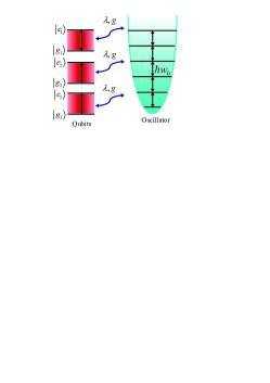
Figure 1: (Color online) Schematic of the system with three identical qubits coupled to a harmonic oscillator. The $j$th ($j=1,2,3$) qubit with one ground ($|g_{j}\rangle$) and one excited states ($|e_{j}\rangle$) is coupled to the oscillator with frequency $w_{0}$, where the qubit-oscillator coupling strength is denoted by $g$ or $\lambda$.

The quantum system we consider here is that three identical qubits couple to a common harmonic oscillator, as shown in Fig. 1. The Hamiltonian of this qubit-oscillator system is written as :

$$\hat{H} = \sum_{j=1}^{3}\hat{H}_{q_{j}}+\hat{H}_{ho}+\hat{H}_{int},$$ (1)

where

$$\hat{H}_{q_{j}} = -\frac{\Delta}{2}\hat{\sigma}_{x_{j}}-\frac{\epsilon}{2}\hat{\sigma}_{z_{j}},$$ (2)

$$\hat{H}_{ho} = \frac{\hat{p}^{2}}{2m}+\frac{1}{2}mw_{0}^{2}\hat{x}^{2},$$ (4)

$$\hat{H}_{int} = g\hat{x}(\hat{\sigma}_{z_{1}}+\hat{\sigma}_{z_{2}}+\hat{\sigma}_{z_{3}}),$$ (6)

$\hat{\sigma}_{x_{j}}$ and $\hat{\sigma}_{z_{j}}$ are the Pauli matrices (with $\hat{\sigma}_{z_{j}}|e_{j}\rangle$ = $|e_{j}\rangle$, $\hat{\sigma}_{z_{j}}|g_{j}\rangle$ = $-|g_{j}\rangle$, $\hat{\sigma}_{x_{j}}|e_{j}\rangle$ = $|g_{j}\rangle$, and $\hat{\sigma}_{x_{j}}|g_{j}\rangle$ = $|e_{j}\rangle$) of the $j$th qubit, where $|e_{j}\rangle$ and $|g_{j}\rangle$ are respectively the excited and ground states of the $j$th qubit, and $\hat{x}$ and $\hat{p}$ are respectively the position and momentum operators of the harmonic oscillator. $\Delta$ and $\epsilon$ are the gap and bias characterizing each qubit. $m$ is the effective mass of the oscillator with frequency $w_{0}$, and $g$ is the coupling strength between each qubit and the oscillator. The parameters $\Delta$, $\epsilon$, and $g$ are assumed to be positive and real for convenience in the paper.

We can also use the creation ($\hat{a}^{\dagger}$) and annihilation ($\hat{a}$) operators to express the oscillator’s Hamiltonian for convenience :

$$\hat{H}_{ho} = \hbar w_{0}\hat{a}^{\dagger}\hat{a},$$ (7)

$$\hat{H}_{int} = \lambda(\hat{a}^{\dagger}+\hat{a})(\hat{\sigma}_{z_{1}}+\hat{\sigma}_{z_{2}}+\hat{\sigma}_{z_{3}}),$$ (9)

where the zero-point energy $\frac{1}{2}\hbar w_{0}$ in $\hat{H}_{ho}$ is omitted, and

$$\hat{a}^{\dagger} = \hat{X}-i\hat{P}=\sqrt{\frac{mw_{0}}{2\hbar}}\hat{x}-i\frac{\hat{p}}{\sqrt{2\hbar mw_{0}}},$$ (10)

$$\hat{a} = \hat{X}+i\hat{P}=\sqrt{\frac{mw_{0}}{2\hbar}}\hat{x}+i\frac{\hat{p}}{\sqrt{2\hbar mw_{0}}},$$ (12)

$$\lambda = \sqrt{\frac{\hbar}{2mw_{0}}}g.$$ (13)

In the basis $\{|e_{j}\rangle,|g_{j}\rangle\}$ of the $j$th qubit, the eigenenergies of $\hat{H}_{q_{j}}$ are $\pm E_{q}/2$, where $E_{q}=\sqrt{\Delta^{2}+\epsilon^{2}}$ is the eigenenergy splitting of the bare qubit, and the energetic excited and ground states are respectively represented by $|\uparrow_{j}\rangle$ and $|\downarrow_{j}\rangle$. The angle $\theta$ is introduced here and defined as $\tan\theta=\epsilon/\Delta$, which denotes the relative size between $\hat{\sigma}_{x_{j}}$ and $\hat{\sigma}_{z_{j}}$ and will be used later. The eigenstates of $\hat{H}_{ho}$ are supposed to be the $n$-photon Fock state $|n\rangle$ ($n=0,1,2,...$) with the corresponding eigenenergy $n\hbar w_{0}$ in the bare oscillator.

Since three qubits are equivalent, the system Hamiltonian $\hat{H}$ is rotationally invariant which leads to a splitting of the eight-dimensional Hilbert space of the qubits into three irreducible components and ensuing degeneracies, on the basis of the formula $\frac{1}{2}\otimes\frac{1}{2}\otimes\frac{1}{2}=\frac{1}{2}\oplus\frac{1}{2}\oplus\frac{3}{2}$ arXiv-1304-2529-2013 . The three-qubit Dicke model is mathematically equivalent to two single-qubit Rabi models and a spin-$3/2$ system. However, this symmetry characteristic does not result in integrability because a spin-$3/2$ system has a four-dimensional state space and the nontrivial eigenstates cannot be labelled by a quantum number arXiv-1304-2529-2013 . We remark that since the merit of our adiabatic-approximation method is to give the intuitive insight into the physics, the collective operators and nontrivial vectors for the qubit states are not used and the symmetry characteristic is included in the degeneracy analysis of eigenstates and eigenenergies after using adiabatic approximation in two following situations.

III Adiabatic approximation for two extreme regimes

In the following section, we focus on exploring the qubit-oscillator system in two extreme regimes that can be analytically treated through the approach of adiabatic approximation.

III.1 High-frequency oscillator

The first extreme situation we study is that the oscillator’s frequency is far larger than the qubit’s eigenenergy splitting (i.e., $\hbar w_{0}>>E_{q}$) as well as the coupling strength (i.e., $\hbar w_{0}>>g,\lambda$), in which the oscillator approximately keeps in its energy eigenstate and adiabatically follows the changes induced by three qubits’ states.

Based on the idea of adiabatic approximation PRL-99-173601-2007 ; PRA-81-042311-2010 , we assume that the $j$th qubit has a well defined value of $\hat{\sigma}_{z_{j}}$, i.e., $\hat{\sigma}_{z_{1}}=\pm 1$, $\hat{\sigma}_{z_{2}}=\pm 1$, and $\hat{\sigma}_{z_{3}}=\pm 1$. For simplicity, we define four collective-state symbols for three qubits: $|A_{+3}\rangle$ ($|A_{-3}\rangle$) represents that three qubits are all in their excited states $|e_{1}e_{2}e_{3}\rangle$ (ground states $|g_{1}g_{2}g_{3}\rangle$); $|A_{+1}\rangle$ represents that one of three qubits is in its ground state and the other two qubits are both in the excited states, i.e., $|e_{1}e_{2}g_{3}\rangle$ or $|e_{1}g_{2}e_{3}\rangle$ or $|g_{1}e_{2}e_{3}\rangle$; $|A_{-1}\rangle$ represents that one of three qubits is in its excited state and the other two qubits are both in the ground states, i.e., $|e_{1}g_{2}g_{3}\rangle$ or $|g_{1}e_{2}g_{3}\rangle$ or $|g_{1}g_{2}e_{3}\rangle$. Therefore, when the qubits are in the state $|A_{\pm 1}\rangle$, the effective Hamiltonian for the oscillator is :

$$\hat{H}_{ho,|A_{\pm 1}\rangle} = \hbar w_{0}\hat{a}^{\dagger}\hat{a}\pm\lambda(\hat{a}^{\dagger}+\hat{a}),$$ (14)

which is the same as that in the system with one qubit and one oscillator PRA-81-042311-2010 .

When the qubits are in the state $|A_{\pm 3}\rangle$, the effective Hamiltonian for the oscillator is :

$$\hat{H}_{ho,|A_{\pm 3}\rangle} = \hbar w_{0}\hat{a}^{\dagger}\hat{a}\pm 3\lambda(\hat{a}^{\dagger}+\hat{a}),$$ (15)

which is interpreted as the original oscillator Hamiltonian with the term of a larger force applied, as compared to that applied in the system of one or two qubits interacting with an oscillator PRA-81-042311-2010 ; PLA-376-2977-2012 . The Hamiltonian in Eqs. (14) and (15) can be respectively transformed into Eqs. (7) and (8) :

$$\hat{H}_{ho,|A_{\pm 1}\rangle} = \hbar w_{0}\hat{a}^{\dagger}_{\pm 1}\hat{a}_{\pm 1}-\frac{\lambda^{2}}{\hbar w_{0}},$$ (16)

$$\hat{H}_{ho,|A_{\pm 3}\rangle} = \hbar w_{0}\hat{a}^{\dagger}_{\pm 3}\hat{a}_{\pm 3}-\frac{9\lambda^{2}}{\hbar w_{0}},$$ (17)

with

$$\hat{a}_{\pm 1} = \hat{a}\pm\frac{\lambda}{\hbar w_{0}},$$ (18)

$$\hat{a}_{\pm 3} = \hat{a}\pm\frac{3\lambda}{\hbar w_{0}}.$$ (19)

The eigenstates of $\hat{H}_{ho,|A_{\pm 1}\rangle}$ and $\hat{H}_{ho,|A_{\pm 3}\rangle}$ are the displaced Fock states PRA-46-4138-1992 :

$$|n_{\pm 1}\rangle = e^{\mp\frac{\lambda}{\hbar w_{0}}(\hat{a}^{\dagger}-\hat{a})}|n\rangle,$$ (20)

$$|n_{\pm 3}\rangle = e^{\mp\frac{3\lambda}{\hbar w_{0}}(\hat{a}^{\dagger}-\hat{a})}|n\rangle,$$ (21)

with the corresponding eigenenergies :

$$E_{o,\pm 1} = n\hbar w_{0}-\frac{\lambda^{2}}{\hbar w_{0}},$$ (22)

$$E_{o,\pm 3} = n\hbar w_{0}-\frac{9\lambda^{2}}{\hbar w_{0}}.$$ (23)

The above results can also be intuitively interpreted as the corresponding harmonic oscillator potentials in the position-momentum picture, as plotted in Fig. 2.

Figure 2: (Color online) Schematic of four displaced oscillators. The horizontal and vertical axises represent the position and displaced oscillator’s eigenenergy $E_{do}$, respectively. Four displaced oscillators are shifted to the left or right from the equilibrium position with a specific constant, where the shift direction is determined by the state of three qubits. The eigenstates (plotted with $n$ no more than $2$) that have the same value of $n$ are degenerate for the states $|A_{\pm 1}\rangle$ (or $|A_{\pm 3}\rangle$), and have the symmetry divided by the origin point in horizontal axis.

The eigenstates of the oscillator slightly rely on the states of three qubits, among which there exists special orthogonality, i.e., $\langle m_{-3}|n_{-3}\rangle$ $=\delta_{mn}$, $\langle m_{-1}|n_{-1}\rangle$ $=\delta_{mn}$, $\langle m_{+1}|n_{+1}\rangle$ $=\delta_{mn}$, $\langle m_{+3}|n_{+3}\rangle$ $=\delta_{mn}$, and

$$\langle m_{+3}|n_{+1}\rangle=\langle m_{+1}|n_{-1}\rangle=\langle m_{-1}|n_{-3}\rangle$$ (24)

(25)

$$=\left\{\begin{array}[]{l}\sqrt{\frac{m!}{n!}}e^{-\frac{2\lambda^{2}}{(\hbar w_{0})^{2}}}(-\frac{2\lambda}{\hbar w_{0}})^{n-m}L_{m}^{n-m}\big{[}(\frac{2\lambda}{\hbar w_{0}})^{2}\big{]},n\geq m,\cr\cr\sqrt{\frac{n!}{m!}}e^{-\frac{2\lambda^{2}}{(\hbar w_{0})^{2}}}(\frac{2\lambda}{\hbar w_{0}})^{m-n}L_{n}^{m-n}\big{[}(\frac{2\lambda}{\hbar w_{0}})^{2}\big{]},m>n,\end{array}\right.$$ (29)

(30)

$$\langle m_{+3}|n_{-1}\rangle=\langle m_{+1}|n_{-3}\rangle$$ (31)

(32)

$$=\left\{\begin{array}[]{l}\sqrt{\frac{m!}{n!}}e^{-\frac{8\lambda^{2}}{(\hbar w_{0})^{2}}}(-\frac{4\lambda}{\hbar w_{0}})^{n-m}L_{m}^{n-m}\big{[}(\frac{4\lambda}{\hbar w_{0}})^{2}\big{]},n\geq m,\cr\cr\sqrt{\frac{n!}{m!}}e^{-\frac{8\lambda^{2}}{(\hbar w_{0})^{2}}}(\frac{4\lambda}{\hbar w_{0}})^{m-n}L_{n}^{m-n}\big{[}(\frac{4\lambda}{\hbar w_{0}})^{2}\big{]},m>n,\end{array}\right.$$ (36)

(37)

$$\langle m_{+3}|n_{-3}\rangle$$ (38)

(39)

$$=\left\{\begin{array}[]{l}\sqrt{\frac{m!}{n!}}e^{-\frac{18\lambda^{2}}{(\hbar w_{0})^{2}}}(-\frac{6\lambda}{\hbar w_{0}})^{n-m}L_{m}^{n-m}\big{[}(\frac{6\lambda}{\hbar w_{0}})^{2}\big{]},n\geq m,\cr\cr\sqrt{\frac{n!}{m!}}e^{-\frac{18\lambda^{2}}{(\hbar w_{0})^{2}}}(\frac{6\lambda}{\hbar w_{0}})^{m-n}L_{n}^{m-n}\big{[}(\frac{6\lambda}{\hbar w_{0}})^{2}\big{]},m>n,\end{array}\right.$$ (43)

where $\delta_{mn}$ is the delta function, and $L_{m}^{n-m}$ and $L_{n}^{m-n}$ are the associated Laguerre polynomials.

Based on the eigenstates of displaced oscillator, we now turn to the qubits of the system. For a special value $n$ in the displaced oscillator’s state, we obtain an effective Hamiltonian for three qubits. There are eight qubit states for each value of $n$, then the effective Hamiltonian $\hat{H}_{q,eff}$ is a $8\times 8$ matrix expanded in the space $\Gamma\equiv\{$ $|\phi_{1}\rangle$, $|\phi_{2}\rangle$, $|\phi_{3}\rangle$, $|\phi_{4}\rangle$, $|\phi_{5}\rangle$, $|\phi_{6}\rangle$, $|\phi_{7}\rangle$, $|\phi_{8}\rangle$ $\}$ $\equiv$ $\{$ $|eee\rangle|n_{+3}\rangle$, $|eeg\rangle|n_{+1}\rangle$, $|ege\rangle|n_{+1}\rangle$, $|gee\rangle|n_{+1}\rangle$, $|egg\rangle|n_{-1}\rangle$, $|geg\rangle|n_{-1}\rangle$, $|gge\rangle|n_{-1}\rangle$, $|ggg\rangle|n_{-3}\rangle$ $\}$. By diagonalizing $\hat{H}_{q,eff}$ in $\Gamma$, we obtain its eigenstates $|\phi_{qj}\rangle$ and eigenenergies $E_{qj}$ ($j=1,2,...,8$):

$$E_{q1} = E_{q2}=E_{q3}=E_{q,+1},$$ (45)

$$|\varphi_{q1}\rangle = |\Phi_{1}(+)\rangle,|\varphi_{q2}\rangle=|\Phi_{2}(+)\rangle,|\varphi_{q3}\rangle=|\Phi_{3}(+)\rangle,$$ (46)

$$E_{q4} = E_{q5}=E_{q6}=E_{q,-1},$$ (48)

$$|\varphi_{q4}\rangle = |\Phi_{1}(-)\rangle,|\varphi_{q5}\rangle=|\Phi_{2}(-)\rangle,|\varphi_{q6}\rangle=|\Phi_{3}(-)\rangle,$$ (49)

$$E_{q7} = E_{q,+3},$$ (51)

$$|\varphi_{q7}\rangle = |\Phi_{4}(+)\rangle,$$ (52)

$$E_{q8} = E_{q,-3},$$ (54)

$$|\varphi_{q8}\rangle = |\Phi_{4}(-)\rangle,$$ (55)

where

$$E_{q,\pm 1} = \pm\frac{\Delta}{2}\sqrt{l^{2}+\tan^{2}\theta},$$ (56)

$$E_{q,\pm 3} = \pm\frac{3\Delta}{2}\sqrt{l^{2}+\tan^{2}\theta},$$ (58)

$$|\Phi_{1}(\pm)\rangle = B(\mp)\big{(}\pm|\phi_{3}\rangle\mp|\phi_{4}\rangle-|\phi_{5}\rangle+|\phi_{6}\rangle\big{)},$$ (60)

$$|\Phi_{2}(\pm)\rangle = B(\mp)\big{(}\pm|\phi_{3}\rangle\mp|\phi_{4}\rangle-|\phi_{5}\rangle+|\phi_{7}\rangle\big{)},$$ (61)

$$|\Phi_{3}(\pm)\rangle = B(\mp)\big{[}|\phi_{1}\rangle-\frac{2\tan\theta}{l}(|\phi_{2}\rangle+|\phi_{3}\rangle)\big{]}$$ (64)

$$+(\frac{\pm 2B(\mp)\tan\theta}{l}-1)|\phi_{4}\rangle$$

$$\mp(B(\mp)\mp\frac{2\tan\theta}{l})|\phi_{5}\rangle+|\phi_{8}\rangle,$$

$$|\Phi_{4}(\pm)\rangle = \frac{\mp(l^{2}+4\tan^{2}\theta)B(\mp)+2l\tan\theta}{l^{2}}|\phi_{1}\rangle$$ (69)

$$+(\frac{\mp 2B(\mp)\tan\theta}{l}+1)(|\phi_{2}\rangle+|\phi_{3}\rangle+|\phi_{4}\rangle)$$

$$\mp B(\mp)(|\phi_{5}\rangle+|\phi_{6}\rangle+|\phi_{7}\rangle)+|\phi_{8}\rangle,$$

$$B(\pm) = \frac{\sqrt{l^{2}+\tan^{2}\theta}\pm\tan\theta}{l},$$ (71)

$$l = e^{-2\lambda^{2}/(\hbar w_{0})^{2}}L_{n}\big{[}(\frac{2\lambda}{\hbar w_{0}})^{2}\big{]}.$$ (73)

Note that if three qubits are in the state $|A_{+1}\rangle$ or $|A_{-1}\rangle$, there are three degenerate eigenstates for $\hat{H}_{q,eff}$ in any given value $n$ of the oscillator. We emphasize that the results discussed here still hold even when $\lambda\geq\hbar w_{0}$ PRA-81-042311-2010 , under which the oscillator can be adjusted adiabatically to the slow processes governed by the gaps of non-degenerate eigenenergies. Especially, both the eigenstates and eigenenergies of $\hat{H}_{q,eff}$ depend on the number of photons $n$ in the oscillator, and the gap between any two non-degenerate eigenenergies decreases as a Gaussian function with increasing $\lambda/(\hbar w_{0})$ which becomes a constant when $\lambda/(\hbar w_{0})$ is large enough, indicating that eight eigenstates in $\Gamma$ decouple with each other.

III.2 High-frequency qubits

The second extreme situation we study is that the eigenenergy splitting $E_{q}$ of each qubit is far larger than $\hbar w_{0}$ and $\lambda$, in which three qubits approximately remain in their energy eigenstates and adiabatically follow the changes induced by the slow oscillator. Similar to the adiabatic approximation discussed in Sec. IIIA, we assume that the oscillator has a well-defined value $x$ of the position operator and deal with the effective Hamiltonian of three qubits PRA-81-042311-2010 :

$$\hat{H}_{hq,eff} = \sum_{j=1}^{3}(-\frac{\Delta}{2}\hat{\sigma}_{x_{j}}-\frac{\epsilon}{2}\hat{\sigma}_{z_{j}})+gx(\hat{\sigma}_{z_{1}}+\hat{\sigma}_{z_{2}}+\hat{\sigma}_{z_{3}}),$$ (74)

for which we obtain the eigenenergies as follows :

$$E_{hq,-3} = -3\sqrt{\frac{\Delta^{2}}{4}+(gx-\frac{\epsilon}{2})^{2}},$$ (76)

$$E_{hq,-1} = -\sqrt{\frac{\Delta^{2}}{4}+(gx-\frac{\epsilon}{2})^{2}}\ \ (\mathrm{triple\ degenerate}),$$ (77)

$$E_{hq,+1} = \sqrt{\frac{\Delta^{2}}{4}+(gx-\frac{\epsilon}{2})^{2}}\ \ (\mathrm{triple\ degenerate}),$$ (78)

$$E_{hq,+3} = 3\sqrt{\frac{\Delta^{2}}{4}+(gx-\frac{\epsilon}{2})^{2}}.$$ (79)

Since the eigenenergies of three high-frequency qubits depend on the position $x$ of the oscillator, we now turn to the oscillator’s effective potentials to gain more transparent physics. Acquiring new contributions from three qubits, the oscillator’s effective potentials are obtained :

$$V_{eff,\pm 1} = \frac{1}{2}mw_{0}^{2}x^{2}\pm\sqrt{\frac{\Delta^{2}}{4}+(gx-\frac{\epsilon}{2})^{2}},$$ (80)

$$V_{eff,\pm 3} = \frac{1}{2}mw_{0}^{2}x^{2}\pm 3\sqrt{\frac{\Delta^{2}}{4}+(gx-\frac{\epsilon}{2})^{2}},$$ (81)

where $V_{eff,\pm 1}$ and $V_{eff,\pm 3}$ correspond to three qubits being in the states $|A_{\pm 1}\rangle$ and $|A_{\pm 3}\rangle$, respectively. We remark that the effective potentials in Eqs. (20) and (21) are no longer the harmonic potentials, and the second terms in Eqs. (20) and (21) represent branches of two kinds of hyperbolas associated with different states of three qubits, but its analytical results are mathematically tough to derive generally. Therefore, we analyze some special cases in the following.

Under the condition $E_{q}>>g|x|$, the effective potentials in Eqs. (20) and (21) can be approximated by:

$$V_{eff,\pm 1} \approx \frac{1}{2}mw_{0}^{2}x^{2}\pm\bigg{(}\frac{\sqrt{\Delta^{2}+\epsilon^{2}}}{2}-\frac{\epsilon gx-g^{2}x^{2}}{\sqrt{\Delta^{2}+\epsilon^{2}}}\bigg{)}$$ (82)

$$= \frac{1}{2}m\tilde{w}^{2}_{0,\pm 1}\bigg{(}x\mp\frac{\epsilon g}{m\tilde{w}^{2}_{0,\pm 1}E_{q}}\bigg{)}^{2}\pm\frac{E_{q}}{2},$$ (84)

$$V_{eff,\pm 3} \approx \frac{1}{2}mw_{0}^{2}x^{2}\pm 3\bigg{(}\frac{\sqrt{\Delta^{2}+\epsilon^{2}}}{2}-\frac{\epsilon gx-g^{2}x^{2}}{\sqrt{\Delta^{2}+\epsilon^{2}}}\bigg{)}$$ (86)

$$= \frac{1}{2}m\tilde{w}^{2}_{0,\pm 3}\bigg{(}x\mp\frac{3\epsilon g}{m\tilde{w}^{2}_{0,\pm 3}E_{q}}\bigg{)}^{2}\pm\frac{3E_{q}}{2},$$ (88)

where

$$\tilde{w}^{2}_{0,\pm 1} = w_{0}^{2}\pm 2\frac{g^{2}}{mE_{q}},$$ (89)

$$\tilde{w}^{2}_{0,\pm 3} = w_{0}^{2}\pm 6\frac{g^{2}}{mE_{q}}.$$ (91)

The oscillator’s effective potentials have two ways of being dependent on the states of three qubits. One way is that the location of the minimum potential deviates from the origin point with a quantity proportional to $\epsilon/E_{q}$. The other way is that the oscillator’s frequency is renormalized depending on different states of three qubits: the oscillator’s effective frequency increases when the number of qubits in the excited state is more than that in the ground state, while the oscillator’s effective frequency is reduced when the number of qubits in the excited state is less than that in the ground state. Note that the variation in the renormalized oscillator’s frequency caused by the state of three qubits is proportional to the difference between the number of qubits in the excited state and that in the ground state, which is impossible in the system of one oscillator with only one qubit PRA-81-042311-2010 .

Especially, when three qubits are in their ground states and

$$\frac{6g^{2}}{mw_{0}^{2}E_{q}}>1,$$ (92)

or one of three qubits is in its excited state and the other two qubits are in the ground states and

$$\frac{2g^{2}}{mw_{0}^{2}E_{q}}>1,$$ (93)

the renormalized frequency in Eq. (24) or (25) is mathematically imaginary, indicating that critical points emerge above which the qubit-oscillator system becomes instable. When $|x|>>\Delta/g,\epsilon/g$, the effective potentials behave well with the following ways:

$$V_{eff,\pm 1} \simeq \frac{1}{2}mw_{0}^{2}x^{2}\pm\big{|}gx-\frac{\epsilon}{2}\big{|},$$ (94)

$$V_{eff,\pm 3} \simeq \frac{1}{2}mw_{0}^{2}x^{2}\pm 3\big{|}gx-\frac{\epsilon}{2}\big{|}.$$ (95)

Therefore, the assumption of three adiabatically adjusting qubits above the critical points is still valid.

To see more abundant contents in the ultrastrong-coupling regime, i.e., above the critical points, we separate the discussions into two parts: $\epsilon=0$ and $\epsilon\neq 0$.

For $\epsilon=0$, the effective potentials in Eqs. (22) and (23) turn into :

$$V_{eff,\pm 1}=\left\{\begin{array}[]{l}\big{(}\frac{1}{2}mw_{0}^{2}\pm\frac{g^{2}}{\Delta}\big{)}x^{2}\pm\frac{\Delta}{2},|x|<<\Delta/g,\\ \cr\frac{1}{2}mw_{0}^{2}x^{2}\pm\big{|}gx\big{|},|x|>>\Delta/g,\end{array}\right.$$ (99)

and

$$V_{eff,\pm 3}=\left\{\begin{array}[]{l}\big{(}\frac{1}{2}mw_{0}^{2}\pm\frac{3g^{2}}{\Delta}\big{)}x^{2}\pm\frac{\Delta}{2},|x|<<\Delta/g,\\ \cr\frac{1}{2}mw_{0}^{2}x^{2}\pm 3\big{|}gx\big{|},|x|>>\Delta/g,\end{array}\right.$$ (103)

respectively. When three qubits are in the state $|A_{-3}\rangle$ and with $6g^{2}>mw_{0}^{2}\Delta$, or in the state $|A_{-1}\rangle$ and with $2g^{2}>mw_{0}^{2}\Delta$, say, above the critical point, $V_{eff,-1}$ or $V_{eff,-3}$ becomes a double-well potential. The locations of the minimum potential can be found through the mathematical derivations $\mathrm{d}V_{eff,-1}/\mathrm{d}x=0$ and $\mathrm{d}V_{eff,-3}/\mathrm{d}x=0$ :

$$x_{0,-1} = \pm\sqrt{\frac{g^{2}}{m^{2}w_{0}^{4}}-\frac{\Delta^{2}}{4g^{2}}},$$ (104)

$$x_{0,-3} = \pm\sqrt{\frac{9g^{2}}{m^{2}w_{0}^{4}}-\frac{\Delta^{2}}{4g^{2}}}.$$ (105)

Above the corresponding critical point, the locations of the minimum potential become :

$$x_{0,-1} \simeq \pm\frac{g}{mw_{0}^{2}},$$ (106)

$$x_{0,-3} \simeq \pm\frac{3g}{mw_{0}^{2}},$$ (107)

with the minimum potential energies :

$$V_{min,-1}=V_{eff,-1}(x_{0,-1})-V_{eff,-1}(0)\approx-\frac{g^{2}}{2mw_{0}^{2}},$$ (108)

(109)

$$V_{min,-3}=V_{eff,-3}(x_{0,-3})-V_{eff,-3}(0)\approx-\frac{9g^{2}}{2mw_{0}^{2}},$$ (110)

and the curvatures for both $V_{eff,-1}$ and $V_{eff,-3}$ are approximately equal to each other :

$$\frac{d^{2}V_{eff,-1}}{dx^{2}}\bigg{|}_{x=\pm x_{0,-1}} \simeq \frac{d^{2}V_{eff,-3}}{dx^{2}}\bigg{|}_{x=\pm x_{0,-3}}\simeq mw_{0}^{2},$$ (112)

which is also equal to that of the free oscillator with $g=0$ and that of the system with one qubit and one oscillator PRA-81-042311-2010 . Based on Eqs. (36) and (37), we can estimate the energy space between the ground state and the first excited state above the corresponding critical point.

For $\epsilon\neq 0$, if the qubit-oscillator system is far below the critical points, from Eqs. (22) and (23), we suggest that $\epsilon$ slightly shifts the locations of the minimum in the single-well potenticals to the left or right; if the qubit-oscillator system is far above the critical points, $\epsilon$ breaks the symmetry in the double-well potentials of the slow oscillator, inducing an energetic tendency to one of the four wells.

IV Numerical Verification

In this section, we perform the exactly numerical simulation for the system with three qubits and an oscillator under special regimes (i.e., $\hbar w_{0}>>E_{q}$ and $\hbar w_{0}<<E_{q}$) to testify their properties of the energy-level spectrum and the ground state. The regime with the resonant situation (i.e., $\hbar w_{0}=E_{q}$) will also be considered.

IV.1 Energy-level spectrum

Figure 3: (Color online) Energy spectrums for lowest thirteen levels under the resonant situation: $\hbar w_{0}$/$E_{q}=1$. The rescaled energy $E_{k}/(\hbar w_{0})$ with $k=1,2,3,...,13$ versus the rescaled coupling strength $\lambda/(\hbar w_{0})$ is plotted: (a) $\theta=0$; (b) $\theta=\pi/6$; (c) $\theta=\pi/3$.

The energies of the lowest thirteen levels versus the qubit-oscillator coupling strength under the resonant situation (i.e., $\hbar w_{0}=E_{q}$) are plotted in Fig. 3. In Fig. 3(a), we find when $\epsilon=\lambda=0$, the ground state is nondegenerate, and degeneracy degrees of the excited state from being low to high correspond to 4, 7, 8, 8, … (the symbol “…” represents 8 all the time as the number of energy level increases which is not plotted here), respectively, and the space between neighboring energy levels is $\hbar w_{0}$. If $\lambda$ increases, the energy levels move up or down, and all energy levels form doubly degenerate including the ground state when $\lambda$ becomes large enough, in which the space between neighboring energy levels is $\hbar w_{0}$ again. This result coincides with the symmetric structure of effective double-well potentials in Sec. IIIB. In Fig. 3 (b) and (c), we see when there is a bias $\epsilon$ (i.e., $\theta\neq 0$) and $\lambda$ is small, the energy levels still keep highly degenerate which is similar to the case of $\epsilon=0$ in Fig. 3(a). However, when $\lambda$ is large enough, the degeneracy of the energy levels vanishes and the space between neighboring energy levels varies with $\epsilon$. This variation in energy level caused by $\epsilon$ indicates the asymmetry structure in effective double-well potentials.

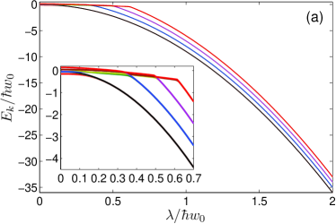
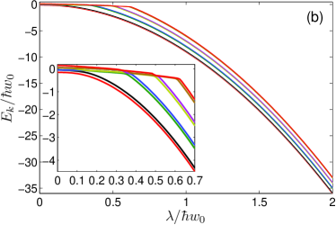
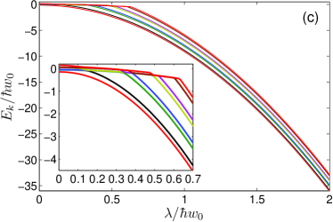
Figure 4: (Color online) Energy spectrums for lowest eight levels under the situation with a high-frequency oscillator: $\hbar w_{0}$/$E_{q}=10$. The rescaled energy $E_{k}/(\hbar w_{0})$ with $k=1,2,3,...,8$ versus the rescaled coupling strength $\lambda/(\hbar w_{0})$ is plotted: (a) $\theta=0$; (b) $\theta=\pi/6$; (c) $\theta=\pi/3$.

In Fig. 4, we plot the spectrums of the lowest eight energy levels versus the qubit-oscillator coupling strength under the situation with a high-frequency oscillator (i.e., $\hbar w_{0}>>E_{q}$). We find that, when $\epsilon=0$, all energy levels form pairs and become doubly degenerate as $\lambda$ becomes large enough, of which the energy gap is $\hbar w_{0}$; when $\epsilon\neq 0$ and $\lambda$ is large enough, the degeneracy in energy-level pairs vanishes and neighboring energy levels are separated by a quantity approximate to $3\epsilon$. This coincides with the result derived in Sec. IIIA. For each value of $n$ and the large-$\lambda$ limit, the oscillator’s effective eigenenergy in Eq. (14) becomes a dominant component in the low energy levels, i.e., three qubits are in the states $|A_{\pm 3}\rangle$ for the large-$\lambda$ limit, producing the effective energy gap $\Delta_{eff}$ $=$ $3\Delta\sqrt{l^{2}+\tan^{2}\theta}\simeq 3\epsilon$ ($l\rightarrow 0$ for large-$\lambda$ limit) in energy-level pairs. This is very different from that in the system of one oscillator with only one qubit PRA-81-042311-2010 , in which the spaces between low energy levels are independent of the bias $\epsilon$.

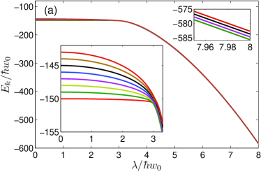
Figure 5: (Color online) Energy spectrums for lowest eight levels under the situation with three high-frequency qubits: $\hbar w_{0}$/$E_{q}=0.01$. The rescaled energy $E_{k}/(\hbar w_{0})$ with $k=1,2,3,...,8$ versus the rescaled coupling strength $\lambda/(\hbar w_{0})$ is plotted: (a) $\theta=0$; (b) $\theta=\pi/6$; (c) $\theta=\pi/3$.

In Fig. 5, we plot the spectrums of the lowest eight energy levels versus the qubit-oscillator coupling strength under the situation with three high-frequency qubits (i.e., $E_{q}>>\hbar w_{0}$). The most interesting effect emerges in the case with $\theta=0$. The ground-state energy maintains constant for $0\leq\lambda\leq\lambda_{c}$, where $\lambda_{c}=\sqrt{\hbar w_{0}\Delta}/(2\sqrt{N_{j}})$ ($N_{j}=3$) is the critical point predicted for a vanishing $\tilde{w}_{0,\pm 3}$. When $\lambda$ $>$ $\lambda_{c}$, the ground-state energy decreases indefinitely with increasing $\lambda$. Especially, the lowest eight energy levels come close to each other with increasing $\lambda$ below the critical point $\lambda_{c}$, and become doubly degenerate when $\lambda$ is beyond $\lambda_{c}$. For the case with $\theta\neq 0$, there is no critical point in the ground-state energy any longer, and the lowest eight energy levels do not form doubly degenerate with increasing $\lambda$, between which the spaces are independent of $\theta$.

IV.2 Properties of ground state

In this section, we analyze the nonclassical properties of the ground state in our qubit-oscillator system under various combinations of system parameters, which are necessary for preparing the oscillator squeezed state, the oscillator Schrödinger-cat state, the qubit-qubit entangled state, and the qubit-oscillator entangled state in the ultrastrong coupling regime.

Figure 6: (Color online) The $Q$ function (upside) and the Wigner function (underside) of the oscillator’s state with three high-frequency qubits (i.e., $\hbar w_{0}/\Delta=0.1$ and $\epsilon=0$): (a,d) $\lambda/(\hbar w_{0})=0.5$, (b,e) $\lambda/(\hbar w_{0})=1$, (c,f) $\lambda/(\hbar w_{0})=1.25$.

We first consider the $Q$ function and Wigner function of the oscillator in the ground state of the qubit-oscillator system. The $Q$ function is defined as :

$$Q(X,P)=\frac{1}{\pi}\langle X-iP|\rho_{osc}|X+iP\rangle,$$ (114)

where $\rho_{osc}=Tr_{q}\{|\Psi_{GS}\rangle\langle\Psi_{GS}|\}$ is the oscillator’s reduced density matrix through tracing out three qubits from the ground state $|\Psi_{GS}\rangle$, and $|X\pm iP\rangle$ represent the coherent states $|\alpha\rangle$ with complex amplitudes $\alpha=X\pm iP$. The Wigner function is defined as :

$$W(X,P) = \frac{1}{2\pi}\int_{-\infty}^{\infty}\langle X+\frac{1}{2}X^{\prime}|\rho_{osc}|X-\frac{1}{2}X^{\prime}\rangle e^{iPX^{\prime}}dX^{\prime},$$ (115)

where $|X\pm\frac{1}{2}X^{\prime}\rangle$ represents the eigenstates of the position operator. We plot the $Q$ and Wigner functions versus parameters $X$ and $P$ under different system parameters in Fig. 6. The results illustrate that the oscillator’s state is initially in a coherent state with no photons (the vacuum state), and becomes a qubit-oscillator entangled state with increasing $\lambda$. The negative value in the Wigner function implies that the nonclassical state of the oscillator, and the nonclassical property of the oscillator becomes more obvious when $\lambda$ increases further, as the obvious interference-fringe-like pattern plotted in Fig. 6(f).

The Schrödinger-cat-like state only appears when two peaks of the Wigner function in Fig. 6 separate completely between which there exist oscillations with alternating positive and negative values, showing the feature of quantum interference. From Fig. 6(e), the nonclassical state of the oscillator first appears when $\lambda\simeq\hbar w_{0}$ in the three-qubit case, which is about one half of that in the single-qubit case PRA-81-042311-2010 . From Fig. 6(f), the minimum qubit-oscillator coupling strength needed to produce the Schrödinger-cat state for our three-qubit Dicke model is $\lambda\simeq 1.25\hbar w_{0}$. However, in the single-qubit case, the minimum qubit-oscillator coupling strength $\lambda$ needed to produce the Schrödinger-cat stat is about $2.5\hbar w_{0}$ PRA-81-042311-2010 , which is about twice as big as that in our three-qubit case. Different from the system of one oscillator with only one qubit PRA-81-042311-2010 , the qubit-oscillator coupling strength needed here for generating the nonclassical states of the Schrödinger-cat type in the oscillator is much smaller, indicating that the qubit-oscillator coupling interaction is collectively enhanced as the number of qubits increases.

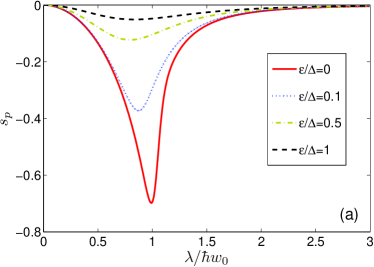
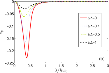
Figure 7: (Color online) The momentum-squeezing parameter $s_{p}$ versus $\lambda/(\hbar w_{0})$: (a) $\hbar w_{0}/\Delta=0.1$, (b) $\hbar w_{0}/\Delta=1$, (c) $\hbar w_{0}/\Delta=10$.

The intuitive quantifier for the squeezing in the oscillator’s state is the set of two squeezing parameters in the $\hat{x}$ and $\hat{p}$ quadratures, given by PRA-81-042311-2010 :

$$s_{p} = 4\langle(\hat{P}-\langle\hat{P}\rangle)^{2}\rangle-1,$$ (117)

$$s_{x} = 4\langle(\hat{X}-\langle\hat{X}\rangle)^{2}\rangle-1,$$ (119)

$$K = \frac{\hbar^{2}}{4}(1+s_{p})(1+s_{x}),$$ (121)

where $K$ equals to $\hbar^{2}/4$ for a minimum-uncertainty state including the coherent and quadrature-squeezed states, while $K$ is larger than $\hbar^{2}/4$ for any other states including the Schrödinger-cat and qubit-oscillator entangled states. The momentum-squeezing parameter versus the qubit-oscillator coupling strength under different system parameters is plotted in Fig. 7. The squeezing in oscillator’s state increases with increasing $\lambda$ for small $\lambda$ and reaches a maximum, but returns to zero as $\lambda$ increases further. This is because the ground state gets entangled in the ultrastrong coupling regime vanishing the squeezing. The maximum attainable squeezing is the biggest under the extreme mechanism $\Delta>>\hbar w_{0}$ and decreases with increasing ratios $\hbar w_{0}/\Delta$ and $\epsilon/\Delta$. We also obtain the numerical results for the parameter $K$, the behaviors of which versus the qubit-oscillator coupling strength are similar to that described in the system of one oscillator with only one qubit PRA-81-042311-2010 .

Based on the above results, we know that the squeezed state can be achieved for moderate qubit-oscillator coupling, and the nonclassical state of the Schrödinger-cat type appears when the Wigner function is negative for relatively strong qubit-oscillator coupling. To make a clear distinction between the Schrödinger-cat state of the oscillator and the qubit-oscillator entangled state, we then take further measures to analyze the properties of the ground-state entanglement.

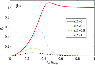
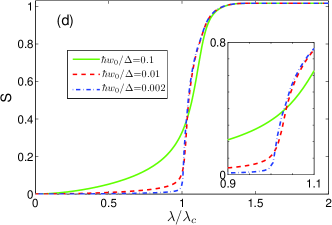
Figure 8: (Color online) The qubits’ entropy $S$ versus $\lambda/(\hbar w_{0})$ with: (a) $\hbar w_{0}/\Delta=0.1$, (b) $\hbar w_{0}/\Delta=1$, (c) $\hbar w_{0}/\Delta=10$. (d) $S$ versus $\lambda/\lambda_{c}$, where $\lambda_{c}$ $=$ $\sqrt{\hbar w_{0}\Delta}/(2\sqrt{3})$ and $\epsilon=0$.

The ground-state entanglement can be quantified by using the von Neumann entropy $S$ of three qubits, which is calculated via the formula $S=-Tr\{\rho_{q}log_{2}\rho_{q}\}$, where $\rho_{q}=Tr_{osc}\{|\Psi_{GS}\rangle\langle\Psi_{GS}|\}$ represents three qubits’ reduced density matrix through tracing out the oscillator degrees of freedom. The entropy of three qubits versus the qubit-oscillator coupling strength is plotted in Fig. 8, which shows when $\epsilon=0$, the entropy increases from zero to a value larger than $1$, and the maximum attainable entropy reaches $1.1$ in Fig. 8(b).

The von Neumann entropy $S$ has a maximum value of $log_{2}D$ in a $D$-dimensional Hilbert space. In the case of three qubits, i.e., an eight-dimensional Hilbert space, the maximum value of qubit-entropy is $S_{max}=3$, which explains the behavior of qubit-entropy being not bounded by $1$ in Fig. 8 meaning three qubits in the ground state can become a nonmaximally entangled state in the limit for large qubit-oscillator coupling. The interaction among these three qubits intermediated by the photons of the oscillator becomes much stronger as the qubit-oscillator coupling strength increases, explaining the increasing behavior of the three-qubit entropy in the ground state without $\epsilon$. This is different from the system of one oscillator with only one qubit PRA-81-042311-2010 , in which the maximum attainable entropy is $1$.

For $\epsilon\neq 0$, the maximum attainable entropy quickly drops to zero as $\lambda$ becomes large enough, and never increases again even when $\lambda$ increases further, indicating the fragility of the ground-state entanglement at such a condition. For the extreme situation with three high-frequency qubits plotted in Fig. 8(d), we assume $\lambda_{c}$ as a reference point for measuring the coupling strength. Interestingly we find that, the onset of the qubits’ entropy becomes suddenly increasing when $\lambda$ is varied across the critical point $\lambda/\lambda_{c}=1$, and the phase-transition-like PRA-81-042311-2010-2 curve in the entropy appears and becomes more sharp as the ratio $\hbar w_{0}/\Delta$ is more close to zero, indicating the system is experiencing a sudden transition from an uncorrelated state to an intensively correlated one as the qubit-oscillator coupling strength increases across the critical point. This phase-transition-like behavior probed by the entropy with only three high-frequency qubits loosens the requirement of employing an atomic ensemble for studying the quantum phase transition PR-93-99-1954 ; PRE-67-066203-2003 ; PRL-90-044101-2003 ; PRL-92-073602-2004 . Note that for non-zero $\epsilon$, one of the wells is “deeper” in Fig. 2, it indeed breaks the parity symmetry of our model and it is this parity that is spontaneously broken in the superradiant phase of the Dicke model.

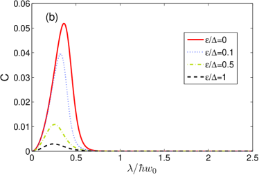
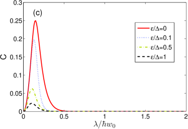
Figure 9: (Color online) The concurrence $C$ for the qubits 2 and 3 versus $\lambda/(\hbar w_{0})$: (a) $\hbar w_{0}/\Delta=0.1$, (b) $\hbar w_{0}/\Delta=1$, (c) $\hbar w_{0}/\Delta=10$.

To investigate the entanglement between any two qubits in the ground state clearly, we use the Wootters’s concurrence $C$ PRL-80-2245-1998 to quantify the entanglement between any two qubits. The concurrence is defined as $C$ $=$ $\max\{$ $0$, $\sqrt{e_{1}}-\sqrt{e_{2}}-\sqrt{e_{3}}-\sqrt{e_{4}}$ $\}$, where $e_{1}$, $e_{2}$, $e_{3}$, and $e_{4}$ are four eigenvalues arranged in decreasing order of the auxiliary matrix $\xi$ $=$ $\rho_{q_{23}}$ $(\sigma_{y}\otimes\sigma_{y})$ $\rho_{q_{23}}^{*}$ $(\sigma_{y}\otimes\sigma_{y})$ (We assume $\rho_{q_{23}}$ $=$ $Tr_{1}\{\rho_{q}\}$ is the reduced density matrix for the qubits 2 and 3) and $\sigma_{y}$ is the corresponding Pauli matrix. The concurrence for the qubits 2 and 3 versus the qubit-oscillator coupling strength is plotted in Fig. 9, which shows: (i) for the small $\lambda$, the concurrence increases with increasing $\lambda$ and reaches to a maximum but then drops rapidly to zero and never increases again as $\lambda$ increases further, meaning the entanglement between any two qubits vanishes if the qubit-oscillator coupling is strong enough; (ii) for $\epsilon=0$, the maximum attainable concurrence is the biggest in the regime $\hbar w_{0}>>\Delta$; and (iii) for $\epsilon\neq 0$, the maximum attainable concurrence decreases with increasing $\epsilon$, demonstrating the fragility of the qubit-qubit entanglement in the ground state.

The numerical results mentioned above demonstrate that the regime $\hbar w_{0}<<E_{q}$ is most suitable for preparing the squeezed states in the oscillator, and the opposite regime $E_{q}>>\hbar w_{0}$ is most proper for generating the entangled states between three qubits and the oscillator. The nonclassical properties of the ground state are analyzed through different intuitive quantifiers, which are demonstrated to be highly susceptible to the variations in the bias parameter.

V Conclusion

We have analytically explored two extreme situations in the system with three qubits interacting with an oscillator by using the approach of adiabatic approximation: one situation considers a high-frequency oscillator and the other one considers three high-frequency qubits. We also numerically calculate the energy spectra and ground-state properties for various combinations of the system parameters which strengthens the outcomes of our analytical derivations based on the adiabatic approximation. The nonclassical properties of the ground state are analyzed through different intuitive quantifiers, which are demonstrated to be highly susceptible to the variations in the bias parameter. Interestingly, we observe the phase-transition-like behaviors in the regime where each qubit’s frequency is far larger than the oscillator’s frequency, and find that the qubit-qubit entanglement in the ground state vanishes if the qubit-oscillator coupling strength is strong enough, in which the entropy of three qubits could keep larger than one. Different from the system of one oscillator with only one qubit, the minimum qubit-oscillator coupling strength needed to produce the Schrödinger-cat state is $1.25\hbar w_{0}$, which is just one half of that in the single-qubit case. The phase-transition-like behavior is also found in the regime where each qubit’s frequency is far larger than the oscillator’s frequency.

VI Acknowledgement

We would like to thank Dr. S. Ashhab and Prof. J. Larson for useful discussions. This work is supported by the Major State Basic Research Development Program of China under Grant No. 2012CB921601, the National Natural Science Foundation of China under Grant No. 11374054, No. 11305037, No. 11347114, and No. 11247283, the Natural Science Foundation of Fujian Province under Grant No. 2013J01012, and the funds from Fuzhou University under Grant No. 022513, Grant No. 022408, and Grant No. 600891.

References

- (1) I. I. Rabi, Phys. Rev. 49, 324 (1936); 51, 652 (1937).
- (2) M. O. Scully and M. S. Zubairy, Quantum Optics (Cambridege University Press, Cambridge, UK, 1997).
- (3) T. Holstein, Ann. Phys. 8, 325 (1959).
- (4) J. M. Raimond, M. Brune, and S. Haroche, Rev. Mod. Phys. 73, 565 (2001).
- (5) D. Leibfried, R. Blatt, C. Monroe, and D. Wineland, Rev. Mod. Phys. 75, 281 (2003).
- (6) E. K. Irish and K. Schwab, Phys. Rev. B 68, 155311 (2003).
- (7) K. Hennessy, A. Badolato, M. Winger, D. Gerace, M. Atatüre, S. Gulde, S. Fält, E. L. Hu, and A. Imamoğlu, Nature 445, 896 (2007).
- (8) D. I. Schuster, A. A. Houck, J. A. Schreier, et al., Nature (London) 445, 515 (2007).
- (9) S. Osnaghi, P. Bertet, A. Auffeves, P. Maioli, M. Brune, J. M. Raimond, and S. Haroche, Phys. Rev. Lett. 87, 037902 (2001).
- (10) S. B. Zheng and G. C. Guo, Phys. Rev. Lett. 85, 2392 (2000).
- (11) E. T. Jaynes and F. W. Cummings, Proc. IEEE 51, 89 (1963).
- (12) A. A. Abdumalikov Jr, O. Astafiev, Y. Nakamura, et al., Phys. Rev. B 78, 180502(R) (2008).
- (13) A. A. Anappara, S. DeLiberato, A. Tredicucci, et al., Phys. Rev. B 79, 201303(R) (2009).
- (14) G. Günter, A. A. Anappara, J. Hees, et al., Nature 458, 178 (2009); P. Forn-Díaz, J. Lisenfeld, D. Marcos, et al., Phys. Rev. Lett. 105, 237001 (2010).
- (15) Y. Todorov, A. M. Andrews, R. Colombelli, et al., Phys. Rev. Lett. 105, 196402 (2010).
- (16) T. Schwartz, J. A. Hutchison, C. Genet, and T. W. Ebbesen, Phys. Rev. Lett. 106, 196405 (2011).
- (17) G. Scalari, C. Maissen, D. Turčinková, et al., Science 335, 1323 (2012).
- (18) A. Crespi, S. Longhi, and R. Osellame, Phys. Rev. Lett. 108, 163601 (2012).
- (19) S. Hayashi, Y. Ishigaki, and M. Fujii, Phys. Rev. B 86, 045408 (2012).
- (20) F. A. Wolf, F. Vallone, G. Romero, M. Kollar, E. Solano, and D. Braak, Phys. Rev. A 87, 023835 (2013).
- (21) X. Cao, J. Q. You, H. Zheng, and F. Nori, New J. Phys. 13, 073002 (2011).
- (22) A. Ridolfo, M. Leib, S. Savasta, and M. J. Hartmann, Phys. Rev. Lett. 109, 193602 (2012).
- (23) C. Ciuti and I. Carusotto, Phys. Rev. A 74, 033811 (2006).
- (24) D. Wang, T. Hansson, Å. Larson, H. O. Karlsson, and J. Larson, Phys. Rev. A 77, 053808 (2008).
- (25) X. F. Cao, J. Q. You, H. Zheng, et al., Phys. Rev. A 82, 022119 (2010).
- (26) V. V. Albert, Phys. Rev. Lett. 108, 180401 (2012).
- (27) R. H. Dicke, Phys. Rev. 93, 99 (1954).
- (28) C. Emary and T. Brandes, Phys. Rev. E 67, 066203 (2003).
- (29) C. Emary and T. Brandes, Phys. Rev. Lett. 90, 044101 (2003).
- (30) N. Lambert, C. Emary, and T. Brandes, Phys. Rev. Lett. 92, 073602 (2004).
- (31) K. Hepp and E. H. Lieb, Ann. Phys. (NY) 76, 360 (1973).
- (32) K. Hepp and E. H. Lieb, Phys. Rev. A 8, 2517 (1973).
- (33) Y. K. Wang and F. T. Hioe, Phys. Rev. A 7, 831 (1973).
- (34) S. B. Zheng, Phys. Rev. A 84, 033817 (2011).
- (35) E. K. Irish, Phys. Rev. Lett. 99, 173601 (2007).
- (36) E. K. Irish, J. Gea-Banacloche, I. Martin, and K. C. Schwab, Phys. Rev. B 72, 195410 (2005).
- (37) H. Zheng, Eur. Phys. J. B 38, 559 (2004).
- (38) H. Chen, Y. M. Zhang, and X. Wu, Phys. Rev. B 40, 11326 (1989).
- (39) J. Stolze and L. Müller, Phys. Rev. B 42, 6704 (1990).
- (40) T. Liu, K. L. Wang, and M. Feng, Eur. Phys. Lett. 86, 54003 (2009).
- (41) D. Zueco, G. M. Reuther, S. Kohler, and P. Hänggi, Phys. Rev. A 80, 033846 (2009).
- (42) J. Casanova, G. Romero, I. Lizuain, J. J. García-Ripoll, and E. Solano, Phys. Rev. Lett. 105, 263603 (2010).
- (43) M. J. Hwang and M. S. Choi, Phys. Rev. A 82, 025802 (2010).
- (44) J. Song, Y. Xia, X. D. Sun, Y. Zhang, B. Liu, and H. S. Song, Eur. Phys. J. D 66, 1 (2012).
- (45) L. X. Yu, et al., Phys. Rev. A 86, 015803 (2012).
- (46) S. Agarwal, S. M. H. Rafsanjani, and J. H. Eberly, Phys. Rev. A 85, 043815 (2012).
- (47) Q. H. Chen, et al., Phys. Rev. A 86, 023822 (2012).
- (48) D. Braak, Phys. Rev. Lett. 107, 100401 (2011).
- (49) Z. G. Lü and H. Zheng, Phys. Rev. B 75, 054302 (2007).
- (50) C. J. Gan and H. Zheng, Eur. Phys. J. D 59, 473 (2010).
- (51) K. M. C. Lee and C. K. Law, Phys. Rev. A 88, 015802 (2013).
- (52) F. Altintas and R. Eryigit, Phys. Rev. A 87, 022124 (2013).
- (53) L. H. Du, X. F. Zhou, Z. W. Zhou, X. Zhou, and G. C. Guo, Phys. Rev. A 86, 014303 (2012).
- (54) H. H. Zhong, Q. T. Xie, and C. H. Lee, J. Phys. A: Math. Theor., 46, 415302 (2013).
- (55) S. A. Chilingaryan and B. M. Rodríguez-Lara, J. Phys. A: Math. Theor. 46, 335301 (2013).
- (56) S. Ashhab and F. Nori, Phys. Rev. A 81, 042311 (2010).
- (57) J. Larson, Euro. Phys. Lett. 90, 54001 (2010).
- (58) J. Larson, J. Phys. B: At. Mol. Opt. Phys. 46, 224016 (2013).
- (59) P. Nataf and C. Ciuti, Phys. Rev. Lett. 107, 190402 (2011). J. Larson, Phys. Scr. 76, 146 (2007).
- (60) D. I. Tsomokos, S. Ashhab, and F. Nori, New J. Phys. 10, 113020 (2010).
- (61) D. Braak, J. Phys. B: At. Mol. Opt. Phys. 46, 224007 (2013).
- (62) L. T. Shen, Z. B. Yang, and R. X. Chen, Phys. Rev. A 88, 045803 (2013).
- (63) S. Ashhab, Phys. Rev. A 87, 013826 (2013).
- (64) T. Niemczyk, F. Deppe, H. Huebl, et al., Nature 6, 772 (2010);
- (65) P. Yang, P. Zhou, and Z. M. Zhang, Phys. Lett. A 376, 2977 (2012).
- (66) M. D. Crisp, Phys. Rev. A 46, 4138 (1992).
- (67) W. K. Wootters, Phys. Rev. Lett. 80, 2245 (1998).