Same universality class for the critical behavior in and out of equilibrium in a quenched random field

Abstract

The random-field Ising model (RFIM) is one of the simplest statistical-mechanical models that captures the anomalous irreversible collective response seen in a wide range of physical, biological, or socio-economic situations in the presence of interactions and intrinsic heterogeneity or disorder. When slowly driven at zero temperature it can display an out-of-equilibrium phase transition associated with critical scaling (“crackling noise”), while it undergoes at equilibrium, under either temperature or disorder-strength changes, a thermodynamic phase transition. We show that the out-of-equilibrium and equilibrium critical behaviors are in the same universality class: they are controlled, in the renormalization-group (RG) sense, by the same zero-temperature fixed point. We do so by combining a field-theoretical formalism that accounts for the multiple metastable states and the exact (functional) RG. As a spin-off, we also demonstrate that critical fluids in disordered porous media are in the same universality class as the RFIM, thereby unifying a broad spectrum of equilibrium and out-of-equilibrium phenomena.

In the presence of both interactions and intrinsic heterogeneity or quenched disorder, a wide spectrum of systems display, when slowly driven by an external solicitation, discrete collective events, bursts, shocks, jerks, or avalanches, that span a broad range of sizes. The signature appears as a “crackling noise”sethna01 and it can be found in quite different situations, sethna01 ; fisher98 ; dahmen-zion from Barkhausen noise in disordered magnetsbertotti to a variety of social and economic phenomenabouchaud13 in passing by capillary condensation in mesoporous materialshallock96 ; detcheverry04 or hysteresis and noise in disordered electron nematics in high-$T_{c}$ superconductors.nematic1 ; nematic2

It has been shown that a simple system such as the random-field Ising model (RFIM) has already all the required ingredients to display crackling noise.sethna93 ; dahmen96 ; sethna05 In this case, the latter results from the presence of an out-of-equilibrium critical point in the hysteretic response of the system to an infinitely slowly changed external field at zero temperature. The critical point separates a phase characterized by finite-size avalanches and a continuous hysteresis curve from a phase with a macroscopic avalanche and a discontinuous hysteresis curve. It requires tuning two control parameters, the disorder strength and the external magnetic field.

On the other hand, the RFIM has been for decades a model for equilibrium phase behavior in the presence of quenched disorder.imry-ma75 ; nattermann98 For dimensions greater than $2$, the RFIM shows a phase transition and a critical point at fixed disorder strength when changing temperature or at fixed temperature when changing disorder strength.nattermann98

The puzzle we address and solve in the present work is the following: despite the fact that one is at equilibrium and the other is not, one is at zero external field and the other is not, and that they take place at different values of the disorder strength, the two types of critical points are characterized by critical exponents and scaling functions that have been found very close in numerical simulations, within numerical accuracy.maritan94 ; perez04 ; liu09 (A similar observation concerning the critical exponents can be made from experiments but the uncertainties are much bigger.)

The theoretical tool for a proper resolution of this puzzle is the renormalization group (RG). The critical behaviors in and out of equilibrium are the same, and are therefore in the same universality class, iff they are controlled by the same RG “fixed point”. (A first piece of information is that the fixed points associated with both types of criticality occur at zero temperature where sample-to-sample fluctuations dominates over thermal ones;villain84 ; fisher86 however, this is a necessary but not sufficient condition.ledoussal-wiese ) A first attempt through an RG formalism was proposed on the basis of perturbation theory.dahmen96 However, the latter is known to seriously fail in the RFIMnattermann98 ; bricmont and cannot provide a useful method. The route we follow here is based on the exact RG and builds on our recent work on the equilibrium behavior of the RFIM.tarjus04 ; tissier11 ; tissier12b

Our demonstration proceeds in several steps. The first one is to replace the a priori complex problem of following a history-dependent evolution among configurations, which results from the dynamics of the slowly driven RFIM, by one that is more readily tackled by statistical mechanical methods. The limit of interest is the adiabatic, or quasi-static, one in which the driving rate is vanishingly slow so that the system reaches a stationary state before being evolved again.sethna93 The trick is that, due to the ferromagnetic nature of the interactions in the RFIM and the properties of the zero-temperature relaxational dynamics (and the associated “no-passing rule”middleton92 ; sethna93 ), the configurations visited along the hysteresis loop correspond to extremal states:guagnelli93 ; mlr10 for a given value of the applied magnetic field (in the language of magnetic systems), they correspond to the stationary states that have the largest local magnetization at each point (for the “descending” branch obtained by decreasing the magnetic field from a fully positively magnetized configuration, see Fig. 1) or the smallest one (for the “ascending branch” obtained by increasing the field from a fully negatively magnetized configuration). When the distribution of the random fields is continuous, which we shall consider, these extremal states are unique for a given realization of the disorder (with exceptional degeneracies).guagnelli93 One can then formulate a statistical mechanical treatment of the extremal states with no reference to dynamics and history.

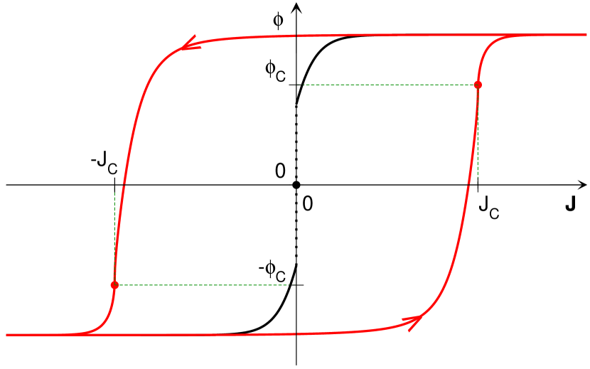
Figure 1: RFIM at zero temperature: Schematic illustration of the hysteresis loop (red) and of the equilibrium curve (blue) in the magnetization ($\phi$) versus applied magnetic field ($J$) representation. For the chosen value of the disorder strength, the system has two (symmetric) out-of-equilibrium critical points (red dots), but a first-order transition in equilibrium.

The model that we consider is the field-theoretical version of the RFIM with short-ranged interactions. The associated “bare action” (microscopic Hamiltonian) is

$$S[\varphi;h+J]=S_{B}[\varphi]-\int_{x}[h(x)+J(x)]\varphi(x)\,,$$ (1)

$$S_{B}[\varphi]=\int_{x}\bigg{\{}\frac{1}{2}[\partial\varphi(x)]^{2}+\frac{r}{2}\varphi(x)^{2}+\frac{u}{4!}\varphi(x)^{4}\bigg{\}},$$

where $\int_{x}\equiv\int d^{d}x$, $h(x)$ is a random “source” (a random magnetic field) and $J(x)$ is an external source (a magnetic field); the quenched random field is taken with a Gaussian distribution characterized by a zero mean and a variance $\overline{h(x)h(y)}=\Delta_{B}\delta^{(d)}(x-y)$.

At zero temperature, the stationary states under consideration are solutions of the stochastic field equation $\frac{\delta S[\varphi;h+J]}{\delta\varphi(x)}=0$. As discussed above, the states that are relevant for the quasi-static hysteresis curve are the two extremal solutions (Fig. 1).

The general recipe to build a generating functional from which one can derive all the needed correlation functions describing the extremal states is (i) to introduce a weighting factor with an auxiliary source linearly coupled to the $\varphi$ field to select the magnetization, and (ii) to consider copies or replicas of the original disordered system, each being independently coupled to distinct external sources.tissier11 ; tissier12b The associated generating functional is then

$$\overline{\mathcal{Z}_{h}[\{\hat{J}_{a},J_{a}\}]}= \int\prod_{a}\mathcal{D}\varphi_{a}\;\overline{\delta\left[\dfrac{\delta S_{B}[\varphi_{a}]}{\delta\varphi_{a}}-h-J_{a}\right]}\;\times$$ (2)

$$\det\left[\dfrac{\delta^{2}S_{B}[\varphi_{a}]}{\delta\varphi_{a}\delta\varphi_{a}}\right]\exp\int_{x}\hat{J}_{a}(x)\varphi_{a}(x)\,,$$

where the overline denotes an average over the Gaussian random field $h(x)$ and square brackets generically indicate functionals.

Note that the above generating functional includes contributions from all solutions of the stochastic field equation (for each copy $a$). However, in the limit where all auxiliary sources $\hat{J}_{a}$ go to infinity, the dominant contribution is that of the extremal states, with maximum magnetization when $\hat{J}_{a}\rightarrow+\infty$ and minimum one when $\hat{J}_{a}\rightarrow-\infty$. The correlation functions are then obtained by first differentiating $\log(\overline{\mathcal{Z}_{h}[\{\hat{J}_{a},J_{a}\}]})$ with respect to the $\hat{J}_{a}$’s and then taking the latter to infinity while considering all $J_{a}$’s equal to $J$. It is worth pointing out the difference with the equilibrium situation at $T=0$. There, the properties of the system are obtained from the ground state, i.e. the solution with minimal action (energy). The ground state can be selected through the introduction of a Boltzmann-like weighting factor with an auxiliary temperature in the limit where the latter is taken to zero.tissier11 ; tissier12b The selection of the extremal states is thus quite different.

To proceed further, as explained in detail in Ref. [tissier11, ], the above functional can be reexpressed with the help of auxiliary fields through standard field-theoretical techniques.Zinn-Justin (1989); Parisi and Sourlas (1979) This leads to a “superfield theory” with a large group of symmetries and supersymmetries.tissier11

The next step consists in applying an exact RG formalism to this superfield theory. This can be done by progressively including the contribution of the fluctuations of the superfield on longer length scales, or alternatively with shorter momenta.wilson74 Technically, this can be implemented through the addition to the bare action of an “infrared (IR) regulator” depending on a running IR scale $k$; its role is to suppress, in the generating functional derived from Eq. (2), the integration over modes with momentum $|q|\lesssim k$.wetterich93 ; Berges et al. (2002); tarjus04

The central quantity of our RG approach is the $k$-dependent “effective average action”,wetterich93 ; Berges et al. (2002) $\Gamma_{k}$. This functional exactly interpolates between the bare action at the microscopic (or UV) scale $k=\Lambda$, which then corresponds to the mean-field approximation where no fluctuations are accounted for, and the exact effective action (Gibbs free energy) when $k=0$. The latter is the generating functional of the so-called “1-particle irreducible” (1PI) correlation functionsZinn-Justin (1989) and its knowledge entails a full description of the statistical properties of the extremal states, hence of the out-of-equilibrium hysteresis behavior of the RFIM. Expanding $\Gamma_{k}$ in increasing number of unrestricted sums over copies (or replicas) generates a cumulant expansion for the renormalized disorder at the scale $k$.tissier11

The RG flow of $\Gamma_{k}$ is generated by continuously decreasing the IR scale $k$. This leads to an exact functional RG equation,wetterich93 ; Berges et al. (2002) from which one derives an exact hierarchy of coupled functional RG equations for the cumulants of the renormalized disorder.

An important simplification occurs in the situation of interest here. As already mentioned, the hysteresis loop corresponds to the limit of infinite auxiliary source, $\hat{J}\rightarrow\pm\infty$, or in the Legendre transformed setting, the limit of infinite auxiliary field, $\hat{\phi}\rightarrow\pm\infty$ ($\hat{\phi}_{a}$ is the average of the auxiliary field introduced as conjugate of the source $J_{a}$ to reexpress Eq. (2)tissier11 ). The main point is that the uniqueness of the extremal states (for each branch separately) translates in the present superfield framework into the formal property of the random generating functional which we called “Grassmannian ultralocality”tissier11 and which greatly simplifies the formalism. A discussion of this property and technical details are provided in the Supplemental Material.A

After some algebra, we end up with exact RG functional equations for the cumulants of the renormalized disorder, $\Gamma_{k1}[\phi_{a}]$, $\Gamma_{k2}[\phi_{a},\phi_{b}]$, etc, or more precisely for the cumulants of the renormalized random field, $\Gamma_{k1;x_{1}}^{(1)}[\phi_{a}]$, $\Gamma_{k2;x_{1},x_{2}}^{(1,1)}[\phi_{a},\phi_{b}]$, etc, with the physical fields $\phi_{a}$ only as arguments (superscripts denote functional differentiation with respect to the arguments). As an illustration, the equation for the first cumulant reads

$$\begin{split}\partial_{t}\Gamma_{k1;x}^{(1)}\left[\phi_{1}\right]=&-\dfrac{1}{2}\tilde{\partial}_{t}\frac{\delta}{\delta\phi_{1}(x)}\int_{x_{2}}\int_{x_{3}}\left(\Gamma_{k1}^{(2)}[\phi_{1}]+\widehat{R}_{k}\right)^{-1}_{x_{2}x_{3}}\\ &\times\bigg{(}\Gamma_{k2;x_{2},x_{3}}^{(11)}\left[\phi_{1},\phi_{1}\right]-\widetilde{R}_{k;x_{2},x_{3}}\bigg{)}\,.\end{split}$$ (3)

where $t=\log(k/\Lambda)$, $\widehat{R}_{k}(q^{2})$ and $\widetilde{R}_{k}(q^{2})$ are IR regulators: $\widehat{R}_{k}(q^{2})$ gives a mass $\sim k^{2}$ for modes with $|q|\lesssim k$ and is essentially zero for modes with $|q|\gtrsim k$, while $\widetilde{R}_{k}(q^{2})$ suppresses fluctuations of the random field and is related to $\widehat{R}_{k}(q^{2})$ in a way that is compatible with the underlying supersymmetry of the theory.tissier11 ; tissier12b Finally, $\widetilde{\partial}_{t}$ is a short-hand notation indicating a derivative with respect to $t$ that acts on the cutoff functions only (i.e., $\widetilde{\partial}_{t}\equiv\partial_{t}\widehat{R}_{k}\,\delta/\delta\widehat{R}_{k}+\partial_{t}\widetilde{R}_{k}\,\delta/\delta\widetilde{R}_{k}$). The auxiliary fields have thus completely dropped out of the equations.

One finds that Eq. (3) coincides with the derivative with respect to $\phi_{1}(x)$ of the exact RG flow equation followed by $\Gamma_{k1}\left[\phi_{1}\right]$ for the RFIM at equilibrium (see Eq. (7) of Ref. [tissier12b, ]). It is easily derived that this generalizes to all higher-order cumulants, so that the exact hierarchies of RG flow equations for the cumulants of the renormalized random field $\Gamma_{kp;x_{1},\cdots,x_{p}}^{(1\cdots 1)}\left[\phi_{1},\cdots,\phi_{p}\right]$ for the RFIM in and out of equilibrium are identical. This is a central result of the present work, and the main ingredient is the uniqueness of the selected stationary states at zero temperature.footnote

We have therefore shown that the out-of-equilibrium hysteresis behavior and the ground-state physics are described by the same exact RG equations. For the equilibrium case, one knows that there exists a fixed point associated with critical behavior. This fixed point has a $Z_{2}$ symmetry, i.e. all functions are symmetric under the inversion of the fields (local magnetizations). It has two relevant directions, one corresponding to a $Z_{2}$ symmetric perturbation and associated with the disorder strength that must be fine-tuned to be exactly at criticality and the other being non $Z_{2}$ symmetric and associated with the external source (which in some sense is also tuned to be zero, which amounts to staying in the $Z_{2}$ symmetric subspace).

The out-of-equilibrium critical point on the other hand has no $Z_{2}$ symmetry: it takes place at nontrivial values of the external source (magnetic field) and of the field (magnetization): $J_{c}>0$, $\phi_{c}\neq 0$ for the ascending branch of the hysteresis loop and, due to the statistical $Z_{2}$ symmetry, $-J_{c}$, $-\phi_{c}$ for the descending branch (see Fig. 1). This implies that the initial condition to the exact RG flow equations, i.e. the mean-field description at the microscopic scale, has no $Z_{2}$ symmetry. (This is akin to the situation encountered when relating the liquid-gas critical point of a genuine fluid that has no particle-hole symmetry to that of the simple Ising model with $Z_{2}$ symmetry.)

To show that non $Z_{2}$ symmetric initial conditions appropriate for describing out-of-equilibrium criticality can flow under RG transformation to the already characterized $Z_{2}$ symmetric equilibrium fixed point, we consider the nonperturbative approximation scheme for the effective average action that we have already introduced in our previous work on the RFIM at equilibrium.tissier11 ; tissier12b It combines a truncation in the “derivative expansion”, i.e. an expansion in the number of spatial derivatives of the fundamental fields for approximating the long-distance behavior of the 1PI correlation functions, and a truncation in the expansion in cumulants of the renormalized disorder. The scheme also ensures that the symmetries and supersymmetries of the theory are not explicitly violated, which turns out to be an important issue for a proper description of “dimensional reduction” and its breakdown.tissier11 ; tissier12b The approximation scheme then leads to a closed set of coupled nonperturbative functional RG equations that can be solved numerically.

When formulated at the level of the cumulants of the renormalized random field, the ansatz takes the form

$$\Gamma_{k1;x_{1}}^{(1)}[\phi]=U^{\prime}_{k}(\phi(x_{1}))+\frac{\delta}{\delta\phi(x_{1})}\big{\{}\frac{1}{2}Z_{k}(\phi(x_{1}))[\partial\phi(x_{1})]^{2}\big{\}}$$ (4)

$$\Gamma_{k2;x_{1},x_{2}}^{(11)}[\phi_{1},\phi_{2}]=\Delta_{k}(\phi_{1}(x_{1}),\phi_{2}(x_{2})),$$

with the higher-order cumulants set to zero. For concreteness, we focus on the critical point along the ascending branch of the hysteresis loop, with $J_{c}>0$. After insertion in the hierarchy of exact RG equations [Eq. (3) and its higher-order counterparts], the above ansatz provides three coupled flow equations for $U^{\prime}_{k}(\phi)$, which describes the renormalized source as a function of magnetization, the so-called “field-renormalization” function $Z_{k}(\phi)$, and the second cumulant of the renormalized random field $\Delta_{k}(\phi_{1},\phi_{2})$.

These flow equations are supplemented by an initial condition at the microscopic (UV) scale $k=\Lambda$. It corresponds to a mean-field approximation where only some coarse-graining over short-ranged fluctuations has been carried out (see e.g. [mlr10, ]). The crucial point is that the bare action has no $Z_{2}$ symmetry around the out-of-equilibrium critical point. The initial condition can then be taken with the same form as in Eq. (LABEL:eq_ansatz) with $Z_{\Lambda}=1$, $\Delta_{\Lambda}=\Delta_{B}$, and $U^{\prime}_{\Lambda}(\phi)$ generically given by $U^{\prime}_{\Lambda}(\phi)=J_{\Lambda}+r_{\Lambda}\phi+\frac{\lambda_{\Lambda}}{2}\phi^{2}+\frac{u_{\Lambda}}{3!}\phi^{3}+\frac{v_{\Lambda}}{4!}\phi^{4}$, where higher-order terms can be dropped as they do not change the universal properties.

To cast the RG flow equations in a dimensionless form that allows one to investigate the critical physics at long length scales, one must introduce scaling dimensions. This is the second operation of any RG transformation. Near a zero-temperature fixed point, the renormalized temperature is irrelevant and is characterized by an exponent $\theta>0$.villain84 ; fisher86 One then has the following scaling dimensions: $Z_{k}\sim k^{-\eta}$, $\phi-\phi_{c}\sim k^{(d-4+\bar{\eta})/2}$, $U^{\prime}_{k}-J_{c}\sim k^{(d-2\eta+\bar{\eta})/2}$, $\Delta_{k}\sim k^{-(2\eta-\bar{\eta})}$, where $\phi_{c}$ and $J_{c}$ respectively denote the values of the magnetization and the magnetic field at the out-of-equilibrium critical point (see above), and the exponents $\theta$, $\eta$ and $\bar{\eta}$ are related through $\theta=2+\eta-\bar{\eta}$.

Due to the lack of $Z_{2}$ inversion symmetry, two relevant parameters must be fine-tuned to reach the critical point. In practice, we account for the additional condition by defining a displaced field variable $\tilde{\phi}=\phi-\phi_{r,k}$ where $\phi_{r,k}$ is fixed such that the third derivative of the renormalized potential is zero all along the flow: $U^{\prime\prime\prime}_{k}(\phi_{r,k})=0$. If indeed the critical system flows to a fixed point where $Z_{2}$ symmetry is restored, then $\phi_{r,k}$ flows to the critical value $\phi_{c}$ and $U^{\prime}_{k}(\phi_{r,k})$ flows to $J_{c}$ in the limit $k\rightarrow 0$.

Using lower-case letters, $u^{\prime\prime}_{k},z_{k},\delta_{k},\tilde{\varphi}$, to denote the dimensionless counterparts of $U^{\prime\prime}_{k},Z_{k},\Delta_{k},\tilde{\phi}$, the dimensionless form of the flow equations can be symbolically written as

$$\begin{split}&\partial_{t}u^{\prime\prime}_{k}(\tilde{\varphi})=\beta_{u^{\prime\prime},k}(\tilde{\varphi}),\;\partial_{t}z_{k}(\tilde{\varphi})=\beta_{z,k}(\tilde{\varphi}),\\ &\partial_{t}\delta_{k}(\tilde{\varphi}_{1},\tilde{\varphi}_{2})=\beta_{\delta,k}(\tilde{\varphi}_{1},\tilde{\varphi}_{2})\,,\end{split}$$ (5)

where the beta functions in the right-hand sides themselves depend on $u^{\prime\prime}_{k}$, $z_{k}$, $\delta_{k}$ and their derivatives. As already stressed above, these flow equations are the same as for the RFIM at equilibrium; they are given in Ref. [tissier12b, ] and not reproduced here.

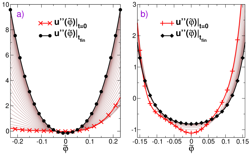
Figure 2: Nonperturbative RG evolution of the dimensionless “mass” function $u^{\prime\prime}_{k}(\tilde{\varphi})$ for $d=5.5>d_{DR}\simeq 5.1$ (a) and $d=4<d_{DR}$ (b). The initial condition (in red) is asymmetric, but the asymmetry gradually decreases along the flow and vanishes at the fixed point (black curve). Furthermore, the fixed-point function for $u^{\prime\prime}_{k}(\tilde{\varphi})$ is identical to that for the equilibrium critical point.

The nonperturbative RG equations can be solved for any spatial dimension $d$ and a variety of initial conditions (yet two parameters must be fine-tuned to reach the critical fixed point). In all cases, we find that the flow leads to the $Z_{2}$ symmetric fixed point already derived for the equilibrium critical point. We illustrate the outcome for two cases (see Fig. 2): one is above the critical dimension for dimensional-reduction breakdown, $d_{DR}\simeq 5.1$,tissier11 ; tissier12b and is therefore exactly described by the $d\rightarrow d-2$ dimensional-reduction property ; the other is below $d_{DR}$ and does not follow dimensional reduction. In both situations, one can clearly see that the asymmetry of $u^{\prime\prime}_{k}(\tilde{\varphi})$ eventually decreases and vanishes when reaching the fixed point. (The same is observed for the other functions $z_{k}(\tilde{\varphi})$ and $\delta_{k}(\tilde{\varphi},\tilde{\varphi})$ but is not displayed here.) The $Z_{2}$ symmetry is thus asymptotically restored and the fixed point exactly coincides with that found for the equilibrium criticality.

The conclusion is that the critical behaviors of the RFIM in and out of equilibrium are in the same universality class, with the same critical exponents, the same scaling functions and the same avalanche-size distribution. This gives a solid theoretical foundation to the empirical numerical findings. Along the way, the above developments also prove that the in- and out-of-equilibrium critical behaviors of fluids in a disordered porous material, which are both described by non $Z_{2}$ symmetric theories,tarjusHRT are in this same universality class. Our present work therefore unifies a very large class of collective phenomena in and out of equilibrium that involve interactions and disorder.

Appendix A Supplemental Material

A.1 Grassmannian ultralocality and exact functional RG equations

As explained in detail in Ref. [tissier11, ], the functional in Eq. (3) of the main text can be reexpressed through standard field-theoretical techniquesZinn-Justin (1989); Parisi and Sourlas (1979) as that of a “superfield theory” with a large group of symmetries and supersymmetries. In a nutshell, one introduces auxiliary (bosonic) fields $\hat{\varphi}_{a}$ to “exponentiate” the delta functional, pairs of auxiliary (fermionic) fields $\psi_{a},\bar{\psi}_{a}$ to “exponentiate” the determinant and one averages over the Gaussian random field.Parisi and Sourlas (1979) By a Legendre transform, one then obtains the “effective action” (Gibbs free energy), $\Gamma[\{\Phi_{a}\}]$ where the $\Phi_{a}$’s are now “superfields” leaving in a “superspace” spanned by the $d$-dimensional Euclidean coordinate $x$ and two anti-commuting Grassmann coordinates $\theta,\bar{\theta}$:Parisi and Sourlas (1979); Zinn-Justin (1989); tissier11

$$\Phi_{a}(x,\theta,\bar{\theta})=\phi_{a}(x)+\bar{\theta}\Psi_{a}(x)+\bar{\Psi}_{a}(x)\theta+\bar{\theta}\theta\hat{\phi}_{a}(x)\,,$$ (6)

where $\phi_{a}(x),\Psi_{a}(x),\bar{\Psi}_{a}(x),\hat{\phi}_{a}(x)$ denote the averages of the physical field and of the associated auxiliary fields in copy $a$.

After having introduced infrared (IR) regulators, one may define an effective averaged action $\Gamma_{k}[\{\Phi_{a}\}]$ which is the effective action of the system at the scale $k$.wetterich93 ; Berges et al. (2002) Its expansion in increasing number of unrestricted sums over copies generates (modulo some inessential subtletiestissier11 ) the cumulant expansion for the renormalized disorder:

$$\Gamma_{k}\left[\{\Phi_{a}\}\right]=\sum_{a}\mathsf{\Gamma}_{k1}[\Phi_{a}]-\frac{1}{2}\sum_{a,b}\mathsf{\Gamma}_{k2}[\Phi_{a},\Phi_{b}]+\cdots$$ (7)

where $\mathsf{\Gamma}_{p}$ is essentially the $p$th cumulant of the renormalized disorder.tissier11 Such an expansion in increasing number of free sums over copies lead to systematic algebraic manipulations that we have repeatedly used.

As recalled in the main text, the evolution of $\Gamma_{k}[\{\Phi_{a}\}]$ with $k$ is described by an exact functional renormalization-group (RG) equation, from which one can derive a hierarchy of exact functional RG equations for the cumulants. For the sake of illustration, we give below the exact RG equation for the first cumulant:

$$\begin{split}\partial_{t}\mathsf{\Gamma}_{k1}[\Phi_{1}]=&\frac{1}{2}\tilde{\partial}_{t}\text{Tr}\Big{\{}\log\Big{(}\mathsf{\Gamma}_{k1}[\Phi_{1}]+\widehat{R}_{k}I\Big{)}+\Big{(}\mathsf{\Gamma}_{k1}^{(2)}[\Phi_{1}]\\ &+\widehat{R}_{k}I\Big{)}^{-1}\Big{(}\mathsf{\Gamma}_{k2}^{(11)}[\Phi_{1},\Phi_{1}]-\widetilde{R}_{k}I\Big{)}\Big{\}},\end{split}$$ (8)

where $t=\log(k/\Lambda)$, the trace involves summing over copy indices and integrating over superspace, and superscripts denote functional differentiation with respect to the superfield arguments; $I$ is the identity, $I_{(a,\theta_{1},\bar{\theta}_{1})(b,\theta_{2},\bar{\theta}_{2})}=\delta_{ab}\delta_{\bar{\theta}_{1},\bar{\theta}_{2}}\delta_{\theta_{1},\theta_{2}}$, where $\delta_{ab}$ is the Kronecker symbol and due to the anticommuting properties of the Grassmann variables,Zinn-Justin (1989) $\delta_{\bar{\theta}_{1},\bar{\theta}_{2}}\delta_{\theta_{1},\theta_{2}}=(\bar{\theta}_{1}-\bar{\theta}_{2})(\theta_{1}-\theta_{2})$; $\widehat{R}_{k}(q^{2})$ and $\widetilde{R}_{k}(q^{2})$ are IR cutoff functions and $\widetilde{\partial}_{t}$ is a short-hand notation indicating a derivative with respect to $t$ that acts on the cutoff functions only (see the main text).

The above RG equation, and the whole hierarchy for higher-order cumulants, is exact but too formal to be useful as such. A major simplification however occurs when the generating functional is built from a unique stationary state (in each replica), which is expected here in the limit of infinite auxiliary source , $\hat{J}\rightarrow\pm\infty$, or in the Legendre transformed setting, the limit of infinite auxiliary field, $\hat{\phi}\rightarrow\pm\infty$. The uniqueness of the extremal states indeed translates in the present superfield framework in the formal property of the random generating functional that we called “Grassmannian ultralocality”.tissier11 The cumulants are then “ultralocal”, i.e.

$$\mathsf{\Gamma}_{k1}[\Phi_{1}]=\int_{\underline{\theta_{1}}}\Gamma_{k1}[\Phi_{1}(\underline{\theta_{1}})]$$ (9)

$$\mathsf{\Gamma}_{k2}[\Phi_{1},\Phi_{2}]=\int_{\underline{\theta_{1}}}\int_{\underline{\theta_{2}}}\Gamma_{k2}[\Phi_{1}(\underline{\theta_{1}}),\Phi_{2}(\underline{\theta_{2}})]\,,$$

etc, where we have grouped the two Grassmann coordinates $\theta,\bar{\theta}$ in the notation $\underline{\theta}$ and $\int_{\underline{\theta}}\equiv\int\int d\theta d\bar{\theta}$. $\Gamma_{k1}$ $\Gamma_{k2}$, etc, in the right-hand sides only depends on the superfields at the explicitly displayed “local” Grassmann coordinates, hence the name “Grassmannian ultralocality”. (On the other hand, the dependence on the Euclidean coordinates, which is left implicit, is not purely local).

The property of Grassmannian ultralocality is also true for the equilibrium case, where the generating functional is dominated by the ground state which is also unique for a given sample (except, again, for a set of conditions of measure zero); it then greatly simplifies the exact functional RG equations.tissier11 ; tissier12b In the present case, one must however proceed differently. We first differentiate the exact RG equations, such as Eq. (8), in order to obtain RG equations for the cumulants of the renormalized random field, $\mathsf{\Gamma}_{k1;x_{1}\underline{\theta_{1}}}^{(1)}[\Phi_{1}]$, $\mathsf{\Gamma}_{k2;x_{1}\underline{\theta_{1}};x_{2}\underline{\theta_{2}}}^{(11)}[\Phi_{1},\Phi_{2}]$, etc. We next evaluate the latter equations at the (external) Grassmann coordinates $\theta_{a}=\bar{\theta}_{a}=0$, for $a=1,2,\cdots$. After some straightforward algebra, we end up with exact RG functional equations for the cumulants $\Gamma_{kp;x_{1},\cdots,x_{p}}^{(1\cdots 1)}$ with the physical fields $\phi_{a}$ only as arguments. For instance, the equation for the first cumulant is given in Eq. (4) of the main text. These equations exactly coincide with those obtained for the same quantities, after using there the very same property of Grassmannian ultralocality, in the equilibrium case.tissier11

A.2 Non-ultralocal corrections

In the above derivation, we have actually used a short-cut that needs justification. Indeed, we have taken the limit $\hat{\phi}\rightarrow\infty$ before a full account of the fluctuations and the limit $k\rightarrow 0$. The correct procedure is instead to solve the exact RG flow down to $k=0$ for $\hat{\phi}$ very large but finite and then take $\hat{\phi}$ to infinity. For large but finite $\hat{\phi}$, there are corrections to the Grassmannian ultralocality. It can however be checked that these corrections become irrelevant as one approaches the fixed point when $k\rightarrow 0$ and therefore give rise to only subdominant contributions. This is what we discuss now.

We now illustrate the structure of the functional RG flow in the presence of “non-ultralocal” components by looking at the corrections in the first cumulant and assuming that all other cumulants are purely “ultralocal” in both Grassmann and Euclidean coordinates. More specifically, we consider

$$\mathsf{\Gamma}_{k1}[\Phi_{1}]=\int_{\underline{\theta}_{1}}\Big{(}\Gamma_{k1}^{UL}[\Phi_{1}(\underline{\theta}_{1})]+$$ (10)

$$\Gamma_{k1}^{NUL}[\Phi_{1}(\underline{\theta}_{1}),\partial_{\theta_{1}}\Phi_{1}(\underline{\theta}_{1}),\partial_{\bar{\theta}_{1}}\Phi_{1}(\underline{\theta}_{1}),\partial_{\theta_{1}}\partial_{\bar{\theta}_{1}}\Phi_{1}(\underline{\theta}_{1})]\Big{)}$$

where $\Gamma_{k1}^{NUL}$ is non-ultralocal in the Grassmann coordinates (i.e. depends on the derivatives) but ultralocal in the Euclidean coordinates, and for $p\geq 2$,

$$\mathsf{\Gamma}_{kp}[\Phi_{1},...,\Phi_{p}]=$$ (11)

$$\int_{\underline{\theta}_{1}}...\int_{\underline{\theta}_{p}}\int_{x_{1}}...\int_{x_{p}}\Gamma_{kp}^{UL}[\Phi_{1}(x_{1},\underline{\theta}_{1}),...,\Phi_{p}(x_{p},\underline{\theta}_{p})]\,.$$

By virtue of the supersymmetries of the theory, the non-ultralocal part of the first cumulant can be rewritten in terms of components in the following form:

$$\mathsf{\Gamma}_{k1}^{NUL}[\Phi_{1}]= \int_{x}\Big{[}\hat{\phi}_{1}(x)\,\gamma_{k1}(\phi_{1}(x),\hat{\phi}_{1}(x))$$ (12)

$$+\Psi_{1}(x)\bar{\Psi}_{1}(x)\,\gamma_{k1}^{(10)}(\phi_{1}(x),\hat{\phi}_{1}(x))\Big{]}\,.$$

In principle, all manipulations should involve the fermionic fields $\Psi_{1},\bar{\Psi}_{1}$, but it turns out that supersymmetries again lead to simplifications and that the same results are obtained by setting these fields to zero, which we do here to simplify the presentation.

The second functional derivative of the effective average action $\Gamma_{k;(a\underline{\theta}_{1})(a\underline{\theta}_{2})}^{(2)}$ that enters in the functional RG equations can be decomposed astissier11

$$\mathsf{\Gamma}_{k;(a\underline{\theta}_{1})(b\underline{\theta}_{2})}^{(2)}=\widehat{\mathsf{\Gamma}}_{k;a\underline{\theta}_{1}\underline{\theta}_{2}}^{(2)}\delta_{ab}+\widetilde{\mathsf{\Gamma}}_{k;(a\underline{\theta}_{1})(b\underline{\theta}_{2})}^{(2)}$$ (13)

After adding the IR regulators, the “hat” and “tilde” components have the following general structure:

$$\begin{split}\widehat{\mathsf{\Gamma}}_{k;a\underline{\theta}_{1}\underline{\theta}_{2}}^{(2)}&[\{\phi_{a},\hat{\phi}_{a}\}]+\widehat{R}_{k}\delta_{\underline{\theta}_{1}\underline{\theta}_{2}}=\widehat{A}_{k;a}+\bar{\theta}_{1}\theta_{1}\bar{\theta}_{2}\theta_{2}\widehat{B}_{k;a}\\ &+(\bar{\theta}_{1}\theta_{1}+\bar{\theta}_{2}\theta_{2})\widehat{C}_{k;a}-(\bar{\theta}_{1}\theta_{2}+\bar{\theta}_{2}\theta_{1})\widehat{E}_{k;a}\end{split}$$ (14)

$$\widetilde{\mathsf{\Gamma}}_{k;(a\underline{\theta}_{1})(b\underline{\theta}_{2})}^{(2)}[\{\phi_{a},\hat{\phi}_{a}\}]+\widetilde{R}_{k}\delta_{\underline{\theta}_{1}\underline{\theta}_{2}} =\widetilde{A}_{k;ab}+\bar{\theta}_{1}\theta_{1}\bar{\theta}_{2}\theta_{2}\widetilde{B}_{k;ab}$$ (15)

$$+\bar{\theta}_{1}\theta_{1}\widetilde{C}_{k;ab}+\bar{\theta}_{2}\theta_{2}\widetilde{D}_{k;ab}\,,$$

and to the lowest order of the expansions in increasing number of free sums over copiestissier11 (leaving implicit the dependence on the Euclidean coordinates):

$$\widehat{A}_{k;a}[\phi_{a},\hat{\phi}_{a}]=2\gamma_{k1}^{(01)}[\phi_{a},\hat{\phi}_{a}]+\hat{\phi}_{a}\gamma_{k1}^{(02)}[\phi_{a},\hat{\phi}_{a}]$$ (16)

$$\widehat{B}_{k;a}[\phi_{a},\hat{\phi}_{a}]=\hat{\phi}_{a}\widehat{\Gamma}_{k1}^{UL(3)}[\phi_{a}]$$

$$\widehat{C}_{k;a}[\phi_{a},\hat{\phi}_{a}]=$$

$$\widehat{\Gamma}_{k1}^{UL(2)}[\phi_{a}]+\widehat{R}_{k}+\gamma_{k1}^{(01)}[\phi_{a},\hat{\phi}_{a}]+\hat{\phi}_{a}\gamma_{k1}^{(11)}[\phi_{a},\hat{\phi}_{a}]$$

$$\widehat{E}_{k;a}\phi_{a},\hat{\phi}_{a}]=\widehat{\Gamma}_{k1}^{UL(2)}[\phi_{a}]+\widehat{R}_{k}+\gamma_{k1}^{(10)}[\phi_{a},\hat{\phi}_{a}]$$

and

$$\widetilde{A}_{k;ab}[\phi_{a},\hat{\phi}_{a},\phi_{b},\hat{\phi}_{b}]=-\Gamma_{k2}^{UL(11)}[\phi_{a},\phi_{b}]+\widetilde{R}_{k}$$ (17)

$$\widetilde{B}_{k;ab}[\phi_{a},\hat{\phi}_{a},\phi_{b},\hat{\phi}_{b}]=-\Gamma_{k2}^{UL(22)}[\phi_{a},\phi_{b}]$$

$$\widetilde{C}_{k;ab}[\phi_{a},\hat{\phi}_{a},\phi_{b},\hat{\phi}_{b}]=-\hat{\phi}_{a}\Gamma_{k2}^{UL(21)}[\phi_{a},\phi_{b}]$$

$$\widetilde{D}_{k;ab}[\phi_{a},\hat{\phi}_{a},\phi_{b},\hat{\phi}_{b}]=-\hat{\phi}_{b}\Gamma_{k2}^{UL(12)}[\phi_{a},\phi_{b}]\;.$$

The full propagator $\mathcal{P}_{k;(a_{1}\underline{\theta}_{1})(a_{2}\underline{\theta}_{2})}$, which is the inverse of $\mathsf{\Gamma}_{k}^{(2)}+\mathcal{R}_{k}$ (where $\mathcal{R}_{k}$ collects the two IR regulators), has the same structure as in Eqs. (13,14,15) with

$$\begin{split}&\widehat{\mathcal{P}}_{k;a\underline{\theta}_{1}\underline{\theta}_{2}}[\{\phi_{a},\hat{\phi}_{a}\}]=\\ &\widehat{Q}_{k;a}+\bar{\theta}_{1}\theta_{1}\bar{\theta}_{2}\theta_{2}\widehat{S}_{k;a}+(\bar{\theta}_{1}\theta_{1}+\bar{\theta}_{2}\theta_{2})\widehat{P}_{k;a}-(\bar{\theta}_{1}\theta_{2}+\bar{\theta}_{2}\theta_{1})\widehat{T}_{k;a}\end{split}$$ (18)

and an expression similar to Eq. (15) for $\widetilde{\mathcal{P}}_{k;(a\underline{\theta}_{1})(b\underline{\theta}_{2})}[\{\phi_{a},\hat{\phi}_{a}\}]$.

At the lowest order of the expansion in increasing free sums over copies, the components of $\widehat{\mathcal{P}}_{k}$ and $\widehat{\mathsf{\Gamma}}_{k}^{(2)}$ are related by

$$\widehat{Q}_{k}[\phi_{a},\hat{\phi}_{a}]=-\big{(}\widehat{C}_{k}\widehat{C}_{k}-\widehat{A}_{k}\widehat{B}_{k}\big{)}^{-1}\widehat{A}_{k}$$ (19)

$$\widehat{S}_{k}[\phi_{a},\hat{\phi}_{a}]=-\big{(}\widehat{C}_{k}\widehat{C}_{k}-\widehat{A}_{k}\widehat{B}_{k}\big{)}^{-1}\widehat{B}_{k}$$

$$\widehat{P}_{k}[\phi_{a},\hat{\phi}_{a}]=\big{(}\widehat{C}_{k}\widehat{C}_{k}-\widehat{A}_{k}\widehat{B}_{k}\big{)}^{-1}\widehat{C}_{k}$$

$$\widehat{T}_{k}[\phi_{a},\hat{\phi}_{a}]=\widehat{E}_{k}^{-1}\,,$$

where one should keep in mind that the components are operators in Euclidean space.

On the other hand, the “tilde” components of the propagator are obtained at the lowest order of the expansion in free sums over copies from

$$\begin{split}&\widetilde{\mathcal{P}}_{k;(a\underline{\theta}_{1})(b\underline{\theta}_{2})}[\phi_{a},\hat{\phi}_{a},\phi_{b},\hat{\phi}_{b}]=-\int_{\underline{\theta}_{3}}\int_{\underline{\theta}_{4}}\widehat{\mathcal{P}}_{k;\underline{\theta}_{1}\underline{\theta}_{3}}[\phi_{a},\hat{\phi}_{a}]\\ &\times\Big{(}\widetilde{\mathsf{\Gamma}}_{k;\underline{\theta}_{3}\underline{\theta}_{4}}^{(2)}[\phi_{a},\hat{\phi}_{a},\phi_{b},\hat{\phi}_{b}]+\widetilde{R}_{k}\Big{)}\widehat{\mathcal{P}}_{k;\underline{\theta}_{4}\underline{\theta}_{2}}[\phi_{b},\hat{\phi}_{b}]\,.\end{split}$$ (20)

The algebraic manipulations are straightforward but the resulting expressions are too lengthy to be reproduced here. We stress that no approximations are involved in deriving results at the lowest order of the expansion in free sums over copies. The higher orders are not needed.

A.3 Functional RG equations with non-ultralocal corrections

We can now collect the above results and insert them in the exact RG equation for the first cumulant, Eq. (8). This leads to

$$\partial_{t}\mathsf{\Gamma}_{k1}[\Phi_{1}]=$$ (21)

$$\frac{1}{2}\int_{x_{1}x_{2}}\int_{\underline{\theta}_{1},\underline{\theta}_{2}}\Big{\{}\partial_{t}\widetilde{R}_{k}(x_{1}-x_{2})\widehat{\mathcal{P}}_{k;(x_{1},\underline{\theta}_{1})(x_{2},\underline{\theta}_{2})}[\phi_{1},\hat{\phi}_{1}]$$

$$+\partial_{t}\widehat{R}_{k}(x_{1}-x_{2})\,\delta_{\underline{\theta}_{1},\underline{\theta}_{2}}\Big{(}\widehat{\mathcal{P}}_{k;(x_{1},\underline{\theta}_{1})(x_{2},\underline{\theta}_{2})}[\phi_{1},\hat{\phi}_{1}]+$$

$$\widetilde{\mathcal{P}}_{k;(x_{1},\underline{\theta}_{1})(x_{2},\underline{\theta}_{2})}[\phi_{1},\hat{\phi}_{1},\phi_{2},\hat{\phi}_{2}]\Big{)}\Big{\}}\,.$$

After taking a functional derivative with respect to $\Phi_{1}(x,\underline{\theta})$, evaluating the outcome for $\theta=\bar{\theta}=0$ and using Eqs. (LABEL:eq_cumulant_1_nonultralocal_correction,LABEL:eq_cumulant_p_ultralocal, 12), one obtains an explicit RG flow equation for $\Gamma_{k1;x}^{(1)UL}[\phi_{1}]+\gamma_{k1}(\phi_{1}(x),\hat{\phi}_{1}(x))+\hat{\phi}_{1}(x)\gamma_{k1}^{(01)}(\phi_{1}(x),\hat{\phi}_{1}(x))$. To keep the presentation in a reasonable format, we further evaluate the equation for spatially uniform fields $\phi_{1}(x)\equiv\phi_{1},\hat{\phi}_{1}(x)\equiv\hat{\phi}_{1}$, so that it simplifies to

$$\partial_{t}U_{k}^{(1)}(\phi_{1})+\partial_{t}\big{[}\gamma_{k1}(\phi_{1},\hat{\phi}_{1})+\hat{\phi}_{1}\gamma_{k1}^{(01)}(\phi_{1},\hat{\phi}_{1})\big{]}=$$ (22)

$$\frac{1}{2}\frac{\delta}{\delta\hat{\phi}_{1}}\int_{q}\Big{\{}\partial_{t}\widetilde{R}_{k}(q^{2})\widehat{S}_{k}(q^{2})+\partial_{t}\widehat{R}_{k}(q^{2})\Big{(}2\big{[}\widehat{P}_{k}(q^{2})$$

$$-\widehat{T}_{k}(q^{2})\big{]}+2\widehat{S}_{k}(q^{2})\big{[}\Gamma_{k2}^{(11)}(q^{2};\phi_{1},\phi_{1})-\tilde{R}_{k}(q^{2})\big{]}\widehat{P}_{k}(q^{2})$$

$$+2\widehat{Q}_{k}(q^{2})\hat{\phi}_{1}^{2}\Gamma_{k2}^{(22)}(q^{2};\phi_{1},\phi_{1})\widehat{P}_{k}(q^{2})+\big{[}\widehat{Q}_{k}(q^{2})\widehat{S}_{k}(q^{2})$$

$$+\widehat{P}_{k}(q^{2})^{2}\big{]}\hat{\phi}_{1}\big{[}\Gamma_{k2}^{(21)}(q^{2};\phi_{1},\phi_{1})+\Gamma_{k2}^{(12)}(q^{2};\phi_{1},\phi_{1})\big{]}\Big{)}\Big{\}}.$$

where $U_{k}(\phi_{1})$ is the effective average potential, i.e. the component of the first cumulant that is ultralocal in both Euclidean and Grassmann coordinates; $\widehat{P}_{k}(q^{2}),\widehat{Q}_{k}(q^{2}),\widehat{S}_{k}(q^{2}),\widehat{T}_{k}(q^{2})$ are functions of $\phi_{1}$ and $\hat{\phi}_{1}$.

Since we are interested in showing that the non-ultralocal corrections give subdominant corrections near the fixed point the limit $|\hat{\phi}|\rightarrow+\infty$, it is sufficient to consider an expansion in $1/|\hat{\phi}|$. For convenience we choose to study the descending branch of the hysteresis loop with $\hat{J}>0$ and $\hat{\phi}>0$. The non-ultralocal component $\gamma_{k1}(\phi,\hat{\phi})$ has an expansion of the form

$$\gamma_{k1}(\phi,\hat{\phi})=\frac{1}{\hat{\phi}^{p}}\Big{(}X_{k0}(\phi)+\frac{X_{k1}(\phi)}{\hat{\phi}}+\cdots\Big{)}.$$ (23)

with $p>1$.

It is easily realized that when the above expansion is inserted in the functional RG equation, Eq. (LABEL:eq_flow_cum1_2), the right-hand side can also be expanded in powers of $1/\hat{\phi}$ and the flow of the ultralocal function $U_{k}^{UL}(\phi_{1})$ is not affected by the non-ultralocal contributions. This property generalizes to the higher cumulants and to the case where the fields are not uniform in the Euclidean space. This is different from what is encountered in the equilibrium case when, studying the asymptotic dominance of the ground state.tissier11 ; tissier12b Along the same lines, the flow for any $X_{kn}(\phi)$ is independent of the higher order terms of the expansion. For instance, the flow of $X_{k0}(\phi)$ reads

$$\partial_{t}X_{k0}(\phi)|_{\phi}\equiv\beta_{X_{0},k}(\phi)=\frac{1}{2(p-1)}\tilde{\partial}_{t}\int_{q}\Big{\{}X^{\prime\prime}_{k0}(\phi)\times$$ (24)

$$\big{[}\Gamma_{k2}^{(11)}(q^{2};\phi,\phi)-\tilde{R}_{k}(q^{2})\big{]}\widehat{P}_{k}(q^{2})^{2}+2X^{\prime}_{k0}(\phi)\widehat{P}_{k}(q^{2})^{2}\times$$

$$\Big{(}2\widehat{P}_{k}(q^{2})\Gamma_{k1}^{(3)UL}(q^{2};\phi)\big{[}\Gamma_{k2}^{(11)}(q^{2};\phi,\phi)-\tilde{R}_{k}(q^{2})\big{]}-$$

$$\big{[}\Gamma_{k2}^{(21)}(q^{2};\phi,\phi)+\Gamma_{k2}^{(12)}(q^{2};\phi,\phi)\big{]}\Big{)}+3X_{k0}(\phi)\widehat{P}_{k}(q^{2})^{2}\times$$

$$\Big{(}2\widehat{P}_{k}(q^{2})^{2}\Gamma_{k1}^{(3UL)}(q^{2};\phi)^{2}\big{[}\Gamma_{k2}^{(11)}(q^{2};\phi,\phi)-\tilde{R}_{k}(q^{2})\big{]}-\widehat{P}_{k}(q^{2})$$

$$\times\big{[}\Gamma_{k2}^{(21)}(q^{2};\phi,\phi)+\Gamma_{k2}^{(12)}(q^{2};\phi,\phi)\big{]}+2\Gamma_{k2}^{(22)}(q^{2};\phi,\phi)\Big{)}\Big{\}}\,.$$

If $X_{k0}$ is equal to zero at the microscopic scale $\Lambda$, which is the initial condition for the RG flow ($X_{\Lambda 0}=0$), then it is obvious from the above equation that it stays zero all along the flow. The power $p$ of the leading behavior in $1/\hat{\phi}$ in Eq. (23) is thus fixed by the initial condition. The latter is a mean-field-like description, which amounts to an effective zero-dimensional model. In the following we therefore make a detour to study a toy model: the $d=0$ version of the out-of-equilibrium RFIM considered here. This will also prove instructive to elucidate the physics behind the non-ultralocal corrections.

A.4 Zero-dimensional RFIM model

We consider the $d=0$ version of the $\phi^{4}$ theory in a quenched random field defined by Eqs. (1-3) of the main text, i.e.

$$S(\phi;h+J)=\frac{r}{2}\phi^{2}+\frac{u}{4!}\phi^{4}-(J+h)\phi\,,$$ (25)

where $r<0$, so that the extremization equation $\partial S(\phi;h+J)/\partial\phi=-|r|\phi+(u/3!)\phi^{3}-(J+h)=0$ has three solutions for a range of $h+J$ around zero. The partition function in the presence of an auxiliary field $\hat{J}$ has contributions from the three solutions (when present):

$$\mathcal{Z}_{h}(\hat{J},J)=\sum^{3}_{\alpha=1}(-1)^{n_{\alpha}}\mathcal{C}_{\alpha}(h+J)e^{\hat{J}\phi_{\alpha}(h+J)}$$ (26)

where $\mathcal{C}_{\alpha}(h+J)$ is the characteritic function of the interval of $h+J$ over which $\phi_{\alpha}$ exists and $n_{\alpha}$ is the index of the $\alpha$th solution (here, $+1$ for a maximum and $-1$ for a minimum).

Consider again for illustration the descending branch of the hysteresis characterized by the extremal state with maximum magnetization $\phi_{M}(h+J)$ which is obtained when $\hat{J}\rightarrow+\infty$. When $\hat{J}$ is large but not infinite, the generating functional in Eq. (26) is dominated by $\exp[\hat{J}\phi_{M}(h+J)]$ (the maximal state is a minimum). Corrections that do not vanish exponentially with $\hat{J}$ can only occur for the range of $h+J$ where a second solution has a magnetization, say $\phi_{S}$, that is within $1/\hat{\phi}$ of $\phi_{M}$. This takes place in the vicinity of the point $h+J=J^{*}$ and $\phi=\phi^{*}$ where the extremal state (minimum) collapses with the nearby saddle-point (maximum). Then, the disorder average of the logarithm of the generating functional, $\mathcal{\mathcal{missing}}W_{1}(\hat{J},J)=\overline{\ln\mathcal{Z}_{h}(\hat{J},J)}$ is given at leading orders in $\hat{J}$ by

$$\mathcal{W}_{1}(\hat{J},J)-\hat{J}\;\overline{\phi_{M}(h+J)}\sim$$ (27)

$$\int d(\delta h)\frac{e^{-\frac{(\delta h-J+J^{*})^{2}}{2\Delta_{B}}}}{\sqrt{2\pi\Delta_{B}}}\ln(1-e^{-2\hat{J}\sqrt{\frac{2|\delta h|}{u\phi^{*}}}})$$

where the integral over $\delta h=h+J-J^{*}$ is restricted to a finite range around $0$. When $\hat{J}\rightarrow\infty$, this leads to

$$\mathcal{W}_{1}(\hat{J},J)-\hat{J}\;\overline{\phi_{M}(h+J)}\sim\frac{e^{-\frac{(J-J^{*})^{2}}{2\Delta_{B}}}}{\sqrt{2\pi\Delta_{B}}}\frac{1}{\hat{J}^{2}}$$ (28)

From the above behavior one immediately obtains that $\hat{\phi}=\mathcal{W}_{1}^{(01)}(\hat{J},J)\sim\hat{J}+\mathcal{O}(1/\hat{J}^{2})$, $\phi=\mathcal{W}_{1}^{(10)}(\hat{J},J)\simeq\overline{\phi_{M}(h+J)}+\mathcal{O}(1/\hat{J}^{3})$ and that $\mathsf{\Gamma}_{1}(\phi,\hat{\phi})=-\mathcal{W}_{1}(\hat{J},J)+\hat{J}\phi+J\hat{\phi}$ is given by

$$\mathsf{\Gamma}_{1}(\phi,\hat{\phi})=\hat{\phi}\,J_{M}(\phi)+\frac{Y(\phi)}{\hat{\phi}^{2}}+\mathcal{O}(1/\hat{\phi}^{3})$$ (29)

when $\hat{\phi},\hat{J}\rightarrow\infty$, where $J_{M}(\phi)$ is the inverse function of $\overline{\phi_{M}(h+J)}$.

The first term of the right-hand side of Eq. (29) is the contribution that is ultralocal in the Grassmann coordinates and the second one is the dominant non-ultralocal correction (the fermionic fields have been set to zero for simplicity). The latter therefore behaves as $1/\hat{\phi}^{2}$ when $\hat{\phi}\rightarrow\infty$. The same result is valid for the mean-field approximation in general dimension $d$ as it essentially amounts to considering a self-consistent zero-dimensional effective system. This shows that the non-ultralocal contribution at the UV scale $\gamma_{k=\Lambda 1}(\phi,\hat{\phi})$ (see Eqs. (12, 23) above) behaves as $1/\hat{\phi}^{3}$ at large $\hat{\phi}$, i.e. $p=3$.

A.5 Results: irrelevance of non-ultralocal corrections at large distance

To investigate the long-distance physics in the vicinity of the out-of-equilibrium critical point, we must cast the functional RG flow equations in a dimensionless form by using scaling dimensions appropriate for a zero-temperature fixed point. This is described in the main text (and in more detail in Ref. [tissier12b, ]). Accordingly, we define a dimensionless non-ultralocal contribution from $X_{k0}(\phi)=k^{\kappa}\chi_{k0}(\tilde{\varphi})$; the associated beta function in Eq. (LABEL:eq_betax0) similarly scales as $\beta_{X_{0},k}(\phi)=k^{\kappa}\beta_{\chi_{0},k}(\tilde{\varphi})$, so that in dimensionless form,

$$\partial_{t}\chi_{k0}(\tilde{\varphi})|_{\tilde{\varphi}}=-\kappa\chi_{k0}(\tilde{\varphi})+\frac{1}{2}(d-4+\bar{\eta})\tilde{\varphi}\chi_{k0}^{\prime}(\tilde{\varphi})+\beta_{\chi_{0},k}(\tilde{\varphi})\,.$$ (30)

The naive expectation for the scaling of $\hat{\phi}$ is that it behaves as $k^{(d+2\eta-\bar{\eta})/2}$. However, $\hat{\phi}$ should rather be adjusted so that $\hat{J}$ can go to infinity even at the fixed point since this is the way to select the extremal state. As

$$\hat{J}=\frac{\partial\mathsf{\Gamma}_{k1}[\phi,\hat{\phi}]}{\partial\hat{\phi}}\simeq U_{k}^{(2)}(\phi)\,\hat{\phi}$$ (31)

with $U_{k}^{(2)}(\phi)\sim k^{2-\eta}$ near the fixed point, $\hat{\phi}$ should scale as $k^{-(2-\eta)}$. More precisely, we define a constant $\hat{\phi}_{0}$ which asymptotically behaves as $\hat{J}$ and such that $\hat{\phi}$ evolves under the RG flow close to the fixed point as $k^{-(2-\eta)}\hat{\phi}_{0}$. The relevant non-ultralocal quantity to be compared with the ultralocal one, $U_{k}^{(1)}(\phi)=k^{(d-2\eta+\bar{\eta})/2}u_{k}^{\prime}(\tilde{\varphi})$, can thus be expressed as

$$\frac{X_{k0}(\phi)}{\hat{\phi}^{3}}=k^{\omega}\,\frac{\chi_{k0}(\tilde{\varphi})}{\hat{\phi}_{0}^{3}}$$ (32)

with $\omega=\kappa+3(2-\eta)$.

We solve Eq. (30) as an eigenvalue equation by setting $\partial_{t}\chi_{*0}(\tilde{\varphi})=0$ and by using the ultralocal functions already found for the fixed point. The 1-replica functions $u_{*}^{\prime\prime}(\tilde{\varphi})$, $z_{*}(\tilde{\varphi})$, and $\chi_{*0}(\tilde{\varphi})$ are discretized on a grid of $2\times 110+1$ points with a mesh of $\delta\tilde{\varphi}=0.005$, thus giving the range of the field $\tilde{\varphi}$ from $-0.55$ to $0.55$. The 2-replica function, i.e. the second cumulant of the renormalized random field, $\delta_{*}(x,y)$ with $x=(\tilde{\varphi}_{1}+\tilde{\varphi}_{2})/2$ and $x=(\tilde{\varphi}_{1}-\tilde{\varphi}_{2})/2$, is discretized on a trapezoidal grid with a base identical to the domain of the 1-replica functions and a height of $36$ points. The mesh in the second field $y$ is identical to that of the field $x$, $\delta y=\delta x$. (We checked that by doubling the resolution of the mesh, our results change on the $4$th digit and by changing the range of fields, the change is on the $6$th digit.)

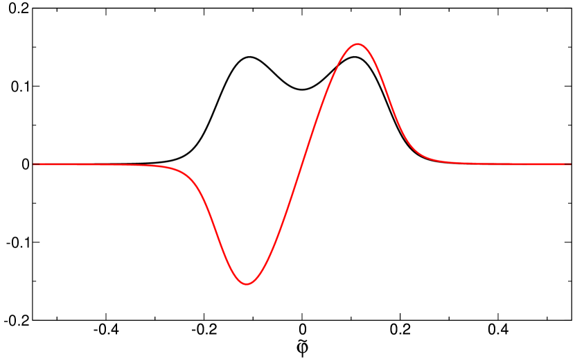
Figure 3: The two nontrivial solutions $\chi_{*0}(\tilde{\varphi})=0$ in $d=4$. One is $Z_{2}$ symmetric and the other one is antisymmetric. In this particular spatial dimension, the corresponding eigenvalues $\kappa_{1}$ and $\kappa_{2}$ are almost identical.

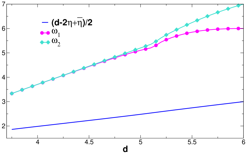
Figure 4: Exponents $\omega_{1}$ (for the $Z_{2}$ symmetric eigenfunction) and $\omega_{2}$ (for the $Z_{2}$ antisymmetric eigenfunction) of the nonultralocal correction as a function of dimension $d$. We also plot the scaling exponent $(d-2\eta+\overline{\eta})/2$ of the corresponding ultralocal term (blue line). It is clear that the non-ultralocal terms are subdominant and do not affect then the universal behavior.

There are two nontrivial solutions of the eigenvalue equation, which are illustrated in Fig. 3 for the dimension $d=4$. The eigenvalues $\kappa_{1,2}$ are monotonically increasing functions of the dimension and they reach at the upper critical dimension $d=6$ values that can be analytically derived: $\kappa_{1}(d=6)=0$ and $\kappa_{2}(d=6)=1$. The eigenvalue $\omega$ defined in Eq. (32) is then simply obtained by adding $3(2-\eta)$. The result is plotted as a function of dimension in Fig. 2. One can clearly see that the exponent of the nonultralocal contribution (whether obtained from the symmetric or the antisymmetric solution) is much larger than that of the ultralocal term. This proves that the corrections to Grassmann ultralocality are irrelevant at large distance, i.e. that the selection of the extremal states is properly ensured.

A.6 Physical interpretation of the non-ultralocal terms

We conclude this material by briefly discussing the physics behind the non-ultralocal corrections. A first hint is given by the zero-dimensional model. As seen in section A.4, the most significant contribution associated with the corrections come from rare situations where the extremal state almost coincides (within $1/\hat{J}$ when $\hat{J}\rightarrow+\infty$) with a nearby saddle-point.

The reasoning can be carried over to the general case. The non-ultralocal corrections are due to rare events where there is an almost degeneracy (within $1/|\hat{J}|$) between the relevant extremal state and a nearby stationary state, solution of the stochastic field equation $\delta S[\varphi;h+J]/\delta\varphi(x)=0$, with a very different configuration yet a very close total magnetization. These rare instances make the non-ultralocal contributions vanish at large distance as a power law rather than the naively anticipated exponential decay. This is somewhat reminiscent of the role of power-law rare “droplet” excitations near the ground state at low but nonzero temperature in the equilibrium case.villain84 ; fisher86 ; tissier08

References

- (1) J. P. Sethna, K. A. Dahmen and C. R. Myers, Nature 410, 242 (2001).
- (2) D. S. Fisher, Phys. Rep. 301, 113 (1998).
- (3) K. A. Dahmen and Y. Ben-Zion, in Extreme Environmental Events R. A. Meyers Ed.(Springer, 2011), p. 5021.
- (4) G. Bertotti, Hysteresis in Magnetism (Academic Press, New york, 1998).
- (5) J.-P. Bouchaud, J. Stat. Phys. 151, 567-606 (2013).
- (6) M. P. Lilly, A. H. Wootters, and R. B. Hallock, Phys. Rev. Lett. 96, 4222 (1996).
- (7) F. Detcheverry et al, Langmuir 20, 8006 (2004).
- (8) J. A. Bonetti et al., Phys. Rev. Lett. 93, 087002 (2004).
- (9) E. W. Carlson et al., Phys. Rev. Lett. 96, 097003 (2006). E. W. Carlson and K. A. Dahmen, Nature Communications 3, 915 (2012).
- (10) J. P. Sethna et al., Phys. Rev. Lett. 70, 3347 (1993).
- (11) J. P. Sethna, K. A. Dahmen and O. Perkovic, in The Science of Hysteresis, edited by G. Bertotti and I. Mayergoyz (Elsevier, Amsterdam, 2005), p. 107.
- (12) K. Dahmen and J.P. Sethna, Phys. Rev. B 53, 14872 (1996).
- (13) Y. Imry and S. K. Ma, Phys. Rev. Lett. 35, 1399 (1975).
- (14) For a review, see T. Nattermann, Spin glasses and random fields (World scientific, Singapore, 1998), p. 277.
- (15) A. Maritan et al., Phys. Rev. Lett. 72, 946 (1994).
- (16) F. J. Perez-Reche and E. Vives, Phys. Rev. B 70, 214422 (2004).
- (17) Y. Liu and K. A. Dahmen, Phys. Rev. E 79, 061124 (2009); Europhys. Lett. 86, 56003 (2009).
- (18) J. Villain, Phys. Rev. Lett. 52, 1543 (1984); J. Physique 46, 1843 (1985).
- (19) D. S. Fisher, Phys. Rev. Lett. 56, 416 (1986).
- (20) P. Le Doussal, K. J. Wiese and P. Chauve, Phys. Rev. B 66, 174201 (2002).
- (21) J. Bricmont and A. Kupiainen, Phys. Rev. Lett 59, 1829 (1987).
- (22) G. Tarjus and M. Tissier, Phys. Rev. Lett 93, 267008 (2004); Phys. Rev. B 78, 024203 (2008).
- (23) M. Tissier and G. Tarjus, Phys. Rev. Lett. 107, 041601 (2011); Phys. B 107, 041601 (2012).
- (24) M. Tissier and G. Tarjus, Phys. B 107, 041601 (2012).
- (25) A. A Middleton, Phys. Rev. Lett. 68, 670 (1992).
- (26) M. Guagnelli, E. Marinari and G. Parisi, J. Phys. A 26, 5675 (1993).
- (27) M.L. Rosinberg and G. Tarjus, J. Stat. Mech., P12011 (2010).
- Zinn-Justin (1989) J. Zinn-Justin, Quantum Field Theory and Critical Phenomena (Oxford University Press, New York, 1989), 3rd ed.
- Parisi and Sourlas (1979) G. Parisi and N. Sourlas, Phys. Rev. Lett. 43, 744 (1979).
- (30) K. G. Wilson and J. Kogut, Phys. Rep. C 12, 77 (1974).
- (31) C. Wetterich, Physics Letters B 301, 90 (1993).
- Berges et al. (2002) J. Berges, N. Tetradis, and C. Wetterich, Phys. Rep. 363, 223 (2002).
- (33) Accordingly, the result is expected to extend to other situations in the RFIM where a unique state is selected by a specific and well defined process, as e.g. for the so-called “demagnetized state”.DMS_carpenter03 ; DMS_colaiori04
- (34) J. H. Carpenter and K. A. Dahmen, Phys. Rev. B 67, 020412 (2003).
- (35) F. Colaiori et al., Phys. Rev. Lett. 92, 257203 (2004).
- (36) G. Tarjus et al., Mol. Phys. 109, 2863 (2013).
- (37) M. Tissier and G. Tarjus, Phys. Rev. B 78, 024204 (2008).