Abstract

We investigate a general relativistic mechanism in which spikes generate matter overdensities in the early universe. When the cosmological fluid is tilted, the tilt provides another mechanism in generating matter inhomogeneities. We numerically investigate the effect of a sign change in the tilt, when there is a spike but the tilt does not change sign, and when the spike and the sign change in the tilt coincide. We find that the tilt plays the primary role in generating matter inhomogeneities, and it does so by creating both local overdensities and underdensities. We discuss of the physical implications of the work.

1 Introduction

As the first step in our effort to explore general relativistic mechanisms that cause spacetime and matter inhomogeneities, in [1] we concentrated on how spikes generate matter overdensities in a radiation fluid in a special class of inhomogeneous models. These spikes occur in the initial oscillatory regime of general cosmological models. The mechanism of spike formation is simple – the state-space orbits of nearby worldlines approach a saddle point; if this collection of orbits straddle the stable manifold of the saddle point, then one of the orbits becomes stuck on the stable manifold of the saddle point and heads towards the saddle point, while the neighbouring orbits leave the saddle point. This heuristic argument holds as long as spatial derivative terms have negligible effect. In the case of spikes, the spatial derivative terms do have a significant effect, and the spike point that initially got stuck does leave the saddle point eventually, and the spike that formed becomes smooth again. In the initial oscillatory regime, spikes recur [2, 3, 4].

With a tilted fluid, the tilt provides another mechanism in generating matter inhomogeneities through the divergence term (in the continuity equation). We will discover that the tilt plays the primary role in generating matter inhomogeneities, but it does so by creating local overdensities and underdensities without particular preference for either one. On the other hand, the spike mechanism plays a secondary role in generating matter inhomogeneities – it drives the divergence term towards making local overdensities.

In this paper we first present the evolution equations of the orthogonally transitive $G_{2}$ model with a perfect fluid, which we will use in the numerical simulations. We briefly review the dynamics of tilt transitions. We then numerically investigate the effect of a sign change in the tilt, which leads to both overdensities and undersities through a large divergence term. We then determine that when there is a complete spike but the tilt does not change sign, the spikes leave a negligible imprint on the matter density. Finally, when the spike and the sign change in the tilt coincide, we find that the spike drives the divergence term towards making overdensities as the universe expands. We conclude that it is the tilt instability that plays the primary role in the formation of matter inhomogeneities. We finish with a discussion of the physical implications of the work.

2 Equations

The model is an orthogonally transitive $G_{2}$ model (also called a Gowdy model) with Killing vector fields acting on a plane, and with a perfect fluid. In order to study the evolution numerically, we use the zooming technique developed in [4] to avoid specifying boundary conditions. The coordinate variable $T$ increases towards the singularity.

We shall omit the derivation of the evolutions equations; for a derivation involving a perfect fluid see [5], and for the derivation involving the zooming technique see [4]. The evolution equations (for our numerical investigation) are:

$$\partial_{T}\ln\beta =-AX\partial_{X}\ln\beta+\frac{3}{2}(1-\Sigma_{+})-\frac{3}{4}(2-\gamma)\frac{1-v^{2}}{G_{+}}\Omega$$ (1)

$$\partial_{T}\ln E_{1}{}^{1} =-AX\partial_{X}\ln E_{1}{}^{1}-1+\frac{3}{4}(2-\gamma)\frac{1-v^{2}}{G_{+}}\Omega$$ (2)

$$\partial_{T}\Sigma_{-} =-AX\partial_{X}\Sigma_{-}+\tfrac{1}{2}{\rm e}^{AT}E_{1}{}^{1}\partial_{X}N_{\times}+\frac{3}{4}(2-\gamma)\frac{1-v^{2}}{G_{+}}\Omega\Sigma_{-}-\sqrt{3}(\Sigma_{\times}^{2}-N_{-}^{2})$$ (3)

$$\partial_{T}N_{\times} =-AX\partial_{X}N_{\times}+\tfrac{1}{2}{\rm e}^{AT}E_{1}{}^{1}\partial_{X}\Sigma_{-}-N_{\times}+\frac{3}{4}(2-\gamma)\frac{1-v^{2}}{G_{+}}\Omega N_{\times}$$ (4)

$$\partial_{T}\Sigma_{\times} =-AX\partial_{X}\Sigma_{\times}-\tfrac{1}{2}{\rm e}^{AT}E_{1}{}^{1}\partial_{X}N_{-}+\frac{3}{4}(2-\gamma)\frac{1-v^{2}}{G_{+}}\Omega\Sigma_{\times}+\sqrt{3}\Sigma_{-}\Sigma_{\times}+\sqrt{3}N_{\times}N_{-}$$ (5)

$$\partial_{T}N_{-} =-AX\partial_{X}N_{-}-\tfrac{1}{2}{\rm e}^{AT}E_{1}{}^{1}\partial_{X}\Sigma_{\times}-N_{-}+\frac{3}{4}(2-\gamma)\frac{1-v^{2}}{G_{+}}\Omega N_{-}-\sqrt{3}\Sigma_{-}N_{-}-\sqrt{3}\Sigma_{\times}N_{\times}$$ (6)

$$\partial_{T}\ln\Omega =-AX\partial_{X}\ln\Omega-\frac{\gamma v}{2G_{+}}{\rm e}^{AT}E_{1}{}^{1}\partial_{X}\ln\Omega+\frac{\gamma G_{-}(1-v^{2})}{2G_{+}^{2}}\partial_{X}{\rm arctanh}v$$

$$\quad-\frac{\gamma}{G_{+}}\left[\frac{G_{+}}{\gamma}(q+1)-\frac{1}{2}(1-3\Sigma_{+})(1+v^{2})-1\right]$$ (7)

$$\partial_{T}{\rm arctanh}v =-AX\partial_{X}{\rm arctanh}v+\frac{(\gamma-1)(1-v^{2})}{2\gamma G_{-}}{\rm e}^{AT}E_{1}{}^{1}\partial_{X}\ln\Omega$$

$$\quad-[3\gamma-4-(\gamma-1)(4-\gamma)v^{2}]\frac{v}{2G_{+}G_{-}}{\rm e}^{AT}E_{1}{}^{1}\partial_{X}{\rm arctanh}v$$

$$\quad+\frac{1}{2\gamma G_{-}}\left[(2-\gamma)G_{+}r-\gamma v(3\gamma-4+3(2-\gamma)\Sigma_{+})\right]$$ (8)

where $\Sigma_{+}$, $q$, $r$, $G_{\pm}$ are given by 

$$\Sigma_{+} =\frac{1}{2}\left(1-\Sigma_{-}^{2}-\Sigma_{\times}^{2}-N_{-}^{2}-N_{\times}^{2}-\Omega\right)$$ (9)

$$q =2-3\Sigma_{+}-\frac{3}{2}(2-\gamma)\frac{1-v^{2}}{G_{+}}\Omega$$ (10)

$$r =-3N_{\times}\Sigma_{-}+3N_{-}\Sigma_{\times}-\frac{3\gamma v}{2G_{+}}\Omega$$ (11)

$$G_{\pm} =1\pm(\gamma-1)v^{2}.$$ (12)

In situations where shock waves develop, we use the upwind method. For upwind method we evolve the variables in two stages using the Godunov splitting – the first stage we evolve only the PDE part, the second stage only the ODE part. Both parts use the timestep $\Delta T$. The second stage uses the new data obtained in the first stage as data at time $T$.  

The first stage requires eigen-functions be evolved using the upwind method. The eigen-functions are

$$\ln\beta,\ \ln E_{1}{}^{1},\ \Sigma_{-}\pm N_{\times},\ \Sigma_{\times}\pm N_{-},\ f_{\pm},$$ (13)

with corresponding eigen-velocities

$$AX,\ AX,\ AX\mp\tfrac{1}{2}{\rm e}^{AT}E_{1}{}^{1},\ AX\pm\tfrac{1}{2}{\rm e}^{AT}E_{1}{}^{1},\ v_{\pm},$$ (14)

where $f_{\pm}$ and $v_{\pm}$ for the perfect fluid are given by

$$f_{\pm}=\ln\left[\frac{1-v^{2}}{G_{+}}\left(\frac{1+v}{1-v}\right)^{\pm\frac{\gamma}{2s}}\Omega\right],$$ (15)

$$v_{\pm}=AX-\tfrac{1}{2}{\rm e}^{AT}E_{1}{}^{1}G_{-}^{-1}\left[(2-\gamma)v\pm s(1-v^{2})\right],$$ (16)

where $s=\sqrt{\gamma-1}$. With these variables, the PDE part of the evolution equations is rewritten as:

$$\partial_{T}\ln\beta =-AX\partial_{X}\ln\beta$$ (17)

$$\partial_{T}\ln E_{1}{}^{1} =-AX\partial_{X}\ln E_{1}{}^{1}$$ (18)

$$\partial_{T}(\Sigma_{-}\pm N_{\times}) =(AX\mp\tfrac{1}{2}{\rm e}^{AT}E_{1}{}^{1})(\Sigma_{-}\pm N_{\times})$$ (19)

$$\partial_{T}(\Sigma_{\times}\pm N_{-}) =(AX\pm\tfrac{1}{2}{\rm e}^{AT}E_{1}{}^{1})(\Sigma_{\times}\pm N_{-})$$ (20)

$$\partial_{T}f_{\pm} =v_{\pm}f_{\pm}$$ (21)

The second stage uses the new data obtained in the first stage as data at time $T$. It evaluates the ODE part of the evolution equations. We shall use the fourth-order Runge-Kutta method. The ODE part of the geometric quantities can be evolved using the original variables

$$\ln\beta,\ \ln E_{1}{}^{1},\ \Sigma_{-},\ N_{\times},\ \Sigma_{\times},\ N_{-}.$$ (22)

Their ODE part is straightforward, for example,

$$\partial_{T}\Sigma_{-}=\frac{3}{4}(2-\gamma)\frac{1-v^{2}}{G_{+}}\Omega\Sigma_{-}-\sqrt{3}(\Sigma_{\times}^{2}-N_{-}^{2})$$ (23)

The ODE part of the evolution equations for perfect fluid is rewritten as:

$$\partial_{T}f_{+} =-\frac{1}{2s(1+sv)}\Big{[}3\gamma(s+v)\Sigma_{+}+2q-(2-\gamma)(1-sv)r$$

$$\quad-\frac{1}{G_{+}}\left(v-2vs^{4}-s+s^{3}-3vs^{2}+3s^{5}v^{2}-v^{3}s^{4}+v^{3}s^{2}+v^{2}s^{3}\right)\Big{]}$$ (24)

$$\partial_{T}f_{-} =-\frac{1}{2s(1-sv)}\Big{[}3\gamma(s-v)\Sigma_{+}+2q+(2-\gamma)(1+sv)r$$

$$\quad-\frac{1}{G_{+}}\left(-v+2vs^{4}-s+s^{3}+3vs^{2}+3s^{5}v^{2}+v^{3}s^{4}-v^{3}s^{2}+v^{2}s^{3}\right)\Big{]}$$ (25)

where $s=\sqrt{\gamma-1}$.

3 Dynamics

Before we present the numerical results, we review some background on tilt transitions [8]. The tilt variable $v$ here in orthogonally transitive $G_{2}$ models is the only remaining nonzero component $v_{1}$ of the velocity of the perfect fluid relative to the observer. $v$ is bounded by -1 and 1. $T$ increases towards big bang singularity.

Linearization of (8) on the Kasner circle with zero tilt gives

$$\partial_{T}v=-\tfrac{1}{2}[3\gamma-4+3(2-\gamma)\Sigma_{+}]v,$$ (26)

which gives the linear solution

$$v=v_{0}e^{-\frac{1}{2}[3\gamma-4+3(2-\gamma)\Sigma_{+}]T}.$$ (27)

Linearization on the Kasner circle with extreme tilt $v^{2}=1$ gives

$$\partial_{T}(1-v^{2})=\tfrac{1}{(2-\gamma)}[3\gamma-4+3(2-\gamma)\Sigma_{+}](1-v^{2}).$$ (28)

Recall that the Hubble-normalized $\Sigma_{+}^{H}$ is given by $\Sigma_{+}^{H}=\Sigma_{+}/(1-\Sigma_{+})$. As $T$ increases, the tilt is unstable on the arc $\Sigma_{+}^{H}<-\tfrac{1}{2}(3\gamma-4)$ of the Kasner circle with zero tilt. See Figure 1. We consider $1\leq\gamma\leq 2$. At the lower bound for $\gamma$, $\Sigma_{+}^{H}<\tfrac{1}{2}$ for dust, which makes the tilt unstable for most of the Kasner epochs (since most of the Kasner epochs are concentrated near $\Sigma_{+}^{H}=-1$). At the upper bound for $\gamma$, $\Sigma_{+}^{H}<-1$ for the stiff fluid. But since $\Sigma_{+}^{H}\geq-1$ by the Gauss constraint, the tilt is always stable for the stiff fluid. For the numerical simulations in this paper, we will restrict to the physically relevant case of the radiation fluid ($\gamma=\frac{4}{3}$), where the tilt is unstable for $\Sigma_{+}^{H}<0$. The tilt is still unstable for most of the Kasner epochs in this case. We also note that growth rate near $v^{2}=1$ is larger than that near $v=0$, which will play a role in tendency to form shockwaves near $v^{2}=1$ first. See [5, pages 59-61] for more discussion on tilt instability.

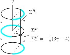
Figure 1: Tilt transitions shown in the state space. The faint arcs on the Kasner circles are unstable towards the singularity.

Based on the above knowledge, it is expected that, in the absence of other transitions, an initial value $v_{0}(x)$ with a sign change combined with tilt instability will develop (towards singularity) into a step function at the position of sign change [5, pages 143-147].

In the next three sections we begin our investigation by studying the effect of a sign change in the tilt, in the context of diagonal $G_{2}$ models. We will see that the sign change in tilt makes both overdensities and undersities through large divergence term. We then ask the next question – what happens when there is a spike, but the tilt does not change sign? Does the spike leave any imprint on the matter density? We will see that the answer is “negligible”. Finally, what happens when the spike and the sign change in tilt coincide? We will see that spike drives the divergence term towards making overdensities as the universe expands.

4 Sign change in tilt and its role through the divergence term

We shall consider the radiation fluid hereafter. $\beta$ decouples from the system and is irrelevant to the dynamics. We begin our investigation by studying the effect of a sign change in tilt, in the context of diagonal $G_{2}$ models. Consider two numerical simulations with the following initial data (see below):

$$\Sigma_{-}=-\frac{7}{2\sqrt{3}},\ N_{\times}=0=\Sigma_{\times}=N_{-},\ \Omega=10^{-5},\ v=\pm\frac{X}{100},\ E_{1}{}^{1}=2e^{-10},$$ (29)

with the slope of $v$ playing an important role in deciding the sign of the divergence term $\partial_{X}v$ in the evolution of $\Omega$.

We run the simulation towards the singularity. We use 1101 grid points on $X\in[-1.1,1.1]$   and run the simulations from $T=0$ to $T=20$.   The particle horizon of the observer at $X=0$ is located approximately at $X=\pm 1$.

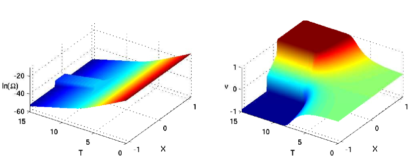
Figure 2: Plots of $\Omega$ and $v$ from the simulation with I.C. (29) with plus sign.

The first initial data with $v=\frac{X}{100}$ gives a positive divergence term, which negates the contribution from the algebraic terms. As a result $\Omega$ develops a local overdensity towards the singularity. See Figures 2 and 3. In this simulation it turns out that the divergence term even dominates the algebraic terms for a brief period and as a result $\Omega$ actually increases towards the singularity during this bried period. Two shockwaves also form. Interpreting this result in the forward time direction (i.e. expanding away from singularity), the positive divergence term means that the fluid flows away from $x=0$, creating a local underdensity as the universe expands.

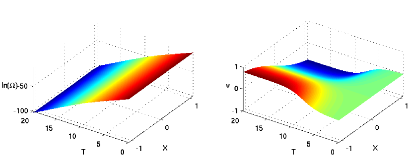
Figure 4: Plots of $\Omega$ and $v$ from the simulation with I.C. (29) with minus sign.

The second initial data with $v=-\frac{X}{100}$ gives a negative divergence term, which adds to the contribution from the algebraic terms. As a result $\Omega$ develops a local underdensity towards the singularity. See Figures 4 and 5. Interpreting this result in the forward time direction, the negative divergence term means that the fluid flows towards $x=0$, creating a local overdensity as the universe expands.

So we see that the divergence term, depending on its sign, can create a local underdensity or overdensity. The tilt instability in the oscillatory regime makes the divergence term larger at surfaces where the tilt changes sign. Also, at shock surfaces, the divergence term is very large. Both $\Omega$ and $v$ develop shockwaves.

The two shockwaves form at surfaces where $v^{2}$ tends to 1 quickly. From the linearized evolution equations (26) and (28) we see that $v^{2}$ tends to 1 at a faster rate than $v$ is leaving 0. This leads to the tendency to form shockwaves near $v^{2}=1$ first.

5 Combining tilt transitions with other transitions

We now shift our attention to orthogonally transitive $G_{2}$ models. Here $\Sigma_{\times}$ and $N_{-}$ are not zero. $N_{-}$ is the trigger for a Bianchi Type II curvature transition; $\Sigma_{\times}$ for a frame transition. A sign change in $N_{-}$ is responsible for a spike transition (and sign change in $\Sigma_{\times}$ for a false spike transition). See [3] for exact solutions and state space diagrams. We focus on the physical transitions, namely the Bianchi Type II transition and the spike transition. How large of a matter inhomogeneity can they generate? To isolate their effect, we study the case without a sign change in the tilt. We use a perturbed spike solution as the initial data

$$(\Sigma_{-},\ N_{\times},\ \Sigma_{\times},\ N_{-})=(-c\Sigma_{-}{}_{\text{Taub}}-\tfrac{1}{\sqrt{3}},\ sN_{-}{}_{\text{Taub}},\ cN_{-}{}_{\text{Taub}},\ -s\Sigma_{-}{}_{\text{Taub}}),\ \Omega=10^{-5},\ v=\tanh(10^{-2}),$$ (30)

where

$$\Sigma_{-}{}_{\text{Taub}}=\tfrac{1}{\sqrt{3}}[\tanh(w(T-T_{0}))-1],\ N_{-}{}_{\text{Taub}}=\tfrac{w}{\sqrt{3}}\text{sech}(w(T-T_{0})),$$ (31)

$$c=\frac{f^{2}-1}{f^{2}+1},\ s=\frac{2f}{f^{2}+1},\ f=we^{T-T_{0}}\text{sech}(w(T-T_{0}))\frac{2}{E_{1}{}^{1}}(X-X_{0}).$$ (32)

We choose the following parameters: $w=1.5$, so that $\Sigma_{-}$ is close to the value $-\frac{7}{2\sqrt{3}}$ in (29); we choose $T=0$, $T_{0}=-10$ so that the spike transition occurs at $T=10$; we choose $E_{1}{}^{1}=2e^{T-T_{0}}$ to cancel out these factors in $f$; and lastly we choose to zoom in on $X_{0}=1$ (away from the spike) and $X_{0}=0$ (at the spike) in two separate simulations. We use 1101 grid points on $X-X_{0}\in[-1.1,1.1]$ and run the simulations from $T=0$ to $T=20$. The particle horizon of the observer at $X=X_{0}$ is located approximately at $X-X_{0}=\pm 1$. The choice $v=10^{-2}$ above is made to avoid a sign change in the tilt, and indeed in the simulations the sign of $v$ remains positive and $v$ tends to $1$.

Zooming in at $X_{0}=0$, the dynamics here is simple – $v$ tends to 1 during $T\in[0,4]$, and then a spike transition occurs during $T\in[6,14]$. $\Omega$ does not develop any observable sub-horizon inhomogeneities. Its value at $T=20$ is $2.748\times 10^{-16}$. See Figure 6.

Zooming in at $X_{0}=1$, the dynamics here is simpler and more homogeneous – $v$ tends to 1 during $T\in[0,4]$, and then a curvature transition and a frame transition occur. The second curvature transition has not occurred before the end of simulation, though its trigger $N_{-}$ is growing slowly. $\Omega$ does not develop any observable sub-horizon inhomogeneities. Its value at $T=20$ is $2.749\times 10^{-16}$. See Figure 7, which is virtually identical to Figure 6.

The plots of $\Omega$ at $T=20$ for the two simulations are compared in Figure 8. We conclude that the spike transition and the curvature transition do not any create observable sub-horizon inhomogeneities, at least when $v^{2}$ is close to 1.

6 Combining sign change in tilt and spike transitions

We now know that a sign change in the tilt generates matter inhomogeneities through the divergence term. But the divergence term can be positive or negative, and has no preference. Do spike transitions influence this preference? To see this, we combine a sign change in the tilt with these transitions. We use the same initial data in (30) except for $v$. Here we use $v=-\tanh(X/100)$, so that initially the divergence term is negative. We zoom in at $X_{0}=0$. We use 1101 grid points on $X-X_{0}\in[-1.1,1.1]$ and run the simulations from $T=0$ to $T=20$. The particle horizon of the observer at $X=X_{0}$ is located approximately at $X-X_{0}=\pm 1$.

Zooming in at $X_{0}=0$, at first $v$ has negative slope, and this slows down the evolution of $v$ towards $\pm 1$. When the spike transition occurs, the expression $-3N_{\times}\Sigma_{-}+3N_{-}\Sigma_{\times}$ in the $r$ term becomes large and drives $v$ in the opposite direction so much so that the slope of $v$ becomes positive. Interpreting this result in the expanding direction, we say that this spike transition alters the slope of $v$ and hence alters the sign of the divergence term from positive to negative. See Figures 9 and 10. Interptreting Figure 10 towards the singularity; $\Omega$ first develops an underdensity, then the expression $-3N_{\times}\Sigma_{-}+3N_{-}\Sigma_{\times}$ becomes large and changes the sign of the divergence term from positive to negative, $\Omega$ now develops an overdensity, and lastly the spike transition takes the solution to the Kasner arc where $v$ is stable and the divergence term becomes small. The initial and final flatness in the plot of $\Omega/\Omega_{\text{side}}$ is an artifact of the initial data at $T=0$ and the fact that the scale of overdensity became super-horizon scale from $T=12$ onwards (because the particle horizon is shrinking). Interpreting Figure 10 forward in time, the overdensity becomes an underdensity at around $T=10$, which then becomes flat (but only because of the initial data we prescribed) at $T=0$. The large expression $-3N_{\times}\Sigma_{-}+3N_{-}\Sigma_{\times}$ at around $T=10$ alters the sign of the divergence term from positive to negative. The negative divergence term undoes the underdensity.

In this case $\Omega$ became essentially homogeneous towards the singularity at subhorizon scale. We saw this in [1] but gave an incorrect interpretation. We incorrectly attributed the primary role of inhomogeneity generation to the spike transition, while it should have been attributed to the sign change in the tilt. Spike transitions play the secondary role of driving the sign of the divergence term towards negative.

Note that although a spike has a ”handedness” to it, the expression $-3N_{\times}\Sigma_{-}+3N_{-}\Sigma_{\times}$ does not. This can be seen by running a similar simulation with $w=-1.5$. This changes the sign of the triggers $N_{-}$ and $\Sigma_{\times}$, but $N_{\times}$ and $\Sigma_{-}$ maintain their signs. From the expression for $r$ we see that $r$ maintains its sign as a result ($r$ is positive for $X>0$). So this spike with $w=-1.5$ still does the same thing to $v$ and the divergence term.

We can conclude that, if $v$ is small (unlike in the previous section where $v^{2}$ is close to 1), then the spike transition manages to drive the divergence term towards negative in the expanding direction. While the divergence term itself has no preference to be positive or negative, spike transitions drive the divergence term towards negative whenever they intersect a sign change of the tilt. In a general model without symmetry, this intersection occurs along curves, and generates local overdensity in the matter along these curves, leading to a web of local overdensity.

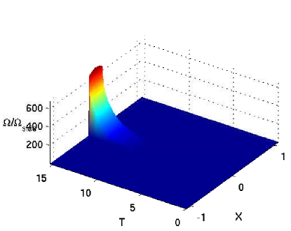
Figure 3: Corresponding ratio $\Omega/\Omega_{X=-1.1}$. $\Omega$ develops an overdensity towards singularity.

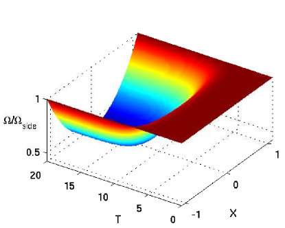
Figure 5: Corresponding ratio $\Omega/\Omega_{X=-1.1}$. $\Omega$ develops an underdensity towards singularity.

Figure 6: Plots of $\Omega$ and $v$ from the simulation with I.C. (30), zooming in at $x=0$.

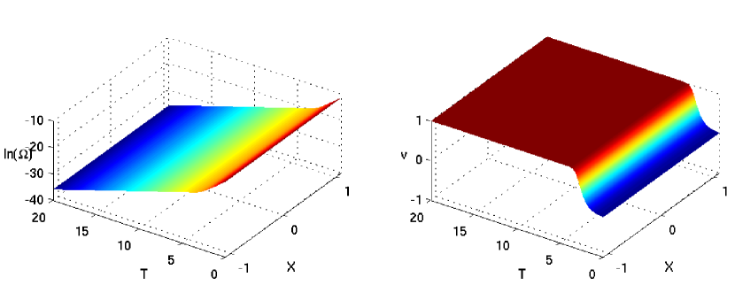
Figure 7: Plots of $\Omega$ and $v$ from the simulation with I.C. (30), zooming in at $x=1$.

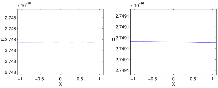
Figure 8: $\Omega$ at $T=20$ for zoom-in at $x=0$ (left panel) and $x=1$, showing that spike alone leaves virtually no imprint on matter.

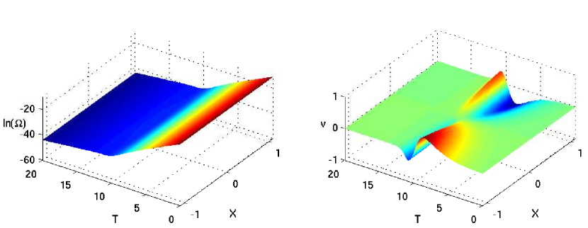
Figure 9: Plots of $\Omega$ and $v$ from the simulation with I.C. (30) but with $v=\tanh(-X/100)$.

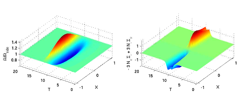
Figure 10: (Left panel) Corresponding ratio $\Omega/\Omega_{X=-1.1}$. $\Omega$ develops first an underdensity and then an overdensity towards singularity. (Right panel) The expression $-3N_{\times}\Sigma_{-}+3N_{-}\Sigma_{\times}$ that drives $v$.

7 Conclusion

In [1] we studied orthogonally transitive $G_{2}$ models with a tilted radiation fluid. We found that spikes, which are purely gravitational inhomogeneities, leave imprints on the radiation fluid in the form of local overdensities. We have obtained further numerical evidence for the existence of GR matter perurbations, which support the results of [1]. However, what we did not realize was that this was partly due to the non-negligible divergence term caused by the instability in the tilt. In this paper we look at the role of the tilt more carefully. We conclude that tilt instability plays the primary role in the formation of matter inhomogeneities. A negative divergence term creates a local overdensity. While the divergence term itself does not prefer one sign or another, spikes drive the divergence term towards negative, creating a web of local overdensities.

We have only explored the orthogonally transitive $G_{2}$ case, which has one tilt degree of freedom. In general there are three tilt degrees of freedom, whose dynamics is even richer. One can imagine that the local overdensities are compressed anisotropically in three different directions, leading to generally elliptical lumps of local overdensities, distributed along surfaces, and with higher densities along intersections of these surfaces. In addition to spikes and large divergence terms, we also encountered shock waves in this paper, but we know almost nothing about the role of these shock waves. Recall that in [1] we discussed incomplete spikes, which have not been studied here. Incompletely spikes, if they terminate before they are halfway done, generate significant local underdensities, provided that they coincide with a non-negligible divergence term.

8 Discussion

In [1] we explicitly showed that in GR spikes naturally occur in a class of $G_{2}$ models leading to inhomogeneities that, due to gravitational instability, leave small residual imprints on matter in the form of matter perturbations. We have shown that the tilt provides another mechanism in generating matter inhomogeneities through the divergence term. In fact, at least in the models we have studied, the tilt plays the primary role in generating matter inhomogeneities, and both overdensities and underdensities are generated.

We are particularly interested in recurring and complete distributed spikes formed in the oscillatory regime (or recurring spikes for short), and their imprint on matter and structure formation. The residual matter overdensities from recurring spikes are not local but form on surfaces. In particular, in the $G_{2}$ models the inhomogeneities can occur on a surface, and in general spacetimes the inhomogeneities can occur along a line, leading to matter inhomogeneities forming on walls or surfaces. Indeed, there are tantalising hints (from dynamical and numerical analyses) that filamentary structures and voids would occur naturally in this scenario.

We have speculated [1] as to whether these recurring spikes might be an alternative to the inflationary mechanism for generating matter perturbations and thus act as seeds for the subsequent formation of large scale structure. Superficially, at least, there are some similarities with perturbations and structure formation created in cosmic string models. The inhomogeneities occur on closed circles or infinite lines [1], similar to what happens in the case of topological defects, and it is expected that a mechanism akin to the Kibble causality mechanicsm will ensure that “defects” form and persist to the present time.

Topological defects, such as domain walls, cosmic strings and global textures, are generically produced during phase transitions in the very early Universe in the framework of (supersymmetric) grand unified theories [9, 10, 11]. The reason why topological defects can play a role in structure formation in the early Universe is because they carry energy which leads to an extra attractive gravitational force, and hence the defects can act as seeds for cosmic structures. In particular, cosmic strings are one-dimensional topological defects which lead to a scale-invariant spectrum of cosmological perturbations (and, among other things, non-Gaussianities) [9, 10, 11]. Cosmic strings contribute to the power spectrum of density fluctuations which affect cosmic microwave background (CMB) radiation temperature anisotropy maps [12, 13, 14]. Although it was shown that cosmic strings (for example) can be ruled out as the unique source of density perturbations leading to the observed structure formation [15, 16], when cosmic strings are included within inflationary models the tension with WMAP and PLANCK data can be reduced [12, 13, 14].

We are also interested in incomplete spikes. Eventually, the oscillatory regime ends when $\Omega$ is no longer negligible, and some of the spikes are in the middle of transitioning, leaving inhomogeneous imprints on the matter result. The residuals from an incomplete spike might, in principle, be large and thus affect structure formation. Indeed, the numerics suggest $\Omega$ develops a void at a spike location [1].

The incomplete spikes associated with Kasner saddle points occur generically in the early universe. Saddles, related to Kasner solutions and FLRW models, may also occur at late times, and may also cause spikes/tilt that might lead to further matter inhomogeneities, albeit non-generically. In particular, since the flat FLRW solution appears to have a 3-dimensional unstable manifold, a spike can still form (towards the future) around a point. This kind of spike is potentially very interesting from the physical point of view. Further investigation is needed to confirm these speculations.

Both the incomplete spikes and the late time non-generic inhomogeneous spikes might lead to the existence of exceptional structures on large scales. In the standard cosmological model spatial homogeneity is only valid on scales larger than 100-115 Mpc [17, 18] (and only then in some statistical sense when averaged on large scales [19, 20, 21, 22, 23]). However, in the actual Universe the distribution of matter is far from homogeneous on scales less than 150-300 Mpc. There are a number of very large structures, such as the Shapley supercluster [24], the Sloan great wall [25], the CfA (great) wall [26] and a number of very large quasar groups (LQGs) [27] and some enormous local voids [28, 29] and void complexes on scales up to 450 Mpc [30].

Such large inhomogeneities in the distribution of superclusters and voids on scales of 200-300 Mpc and above, and especially the “Huge-LQG” (with characteristic volume of size $\sim$ 500 Mpc) and its proximity to the CCLQG at the same redshift ($\sim 1.27$) [27], implies that the Universe is perhaps not homogeneous on these scales, and are potentially in conflict with the cosmological principle and the standard concordance ($\Lambda$CDM) cosmological model [26, 30]). An alternative GR spike mechanism for naturally generating (a small number of) exceptional structures at late times (in additional to the usual distribution of structures produced in the standard model) may resolve some tension with cosmological observations.

Finally, in [31] the existing relationship between polarized Electrogowdy spacetimes and Gowdy spacetimes was exploited to find explicit solutions for electromagnetic spikes. New inhomogeneous solutions, called the electric and the magnetic spike solutions, were presented. It will be interesting to see how gravitational spikes, electromagnetic spikes and perfect fluid interact to generate inhomogeneities in the fluid density and the electromagnetic field. This will provide a relativistic (non-Newtonian and non-quantum) mechanism to produce primodial galaxies and intergalactic magnetic fields, and explain the web-like distribution of these structures. For example, cosmic strings can be responsible for the production of highly energetic bursts of particles, and they can help seed coherent magnetic fields on galactic scales [32]. We will return to this question in the future.

References

- [1] A. A. Coley and W. C. Lim, Phys. Rev. Lett. 108, 191101 (2012), arXiv:1205.2142.
- [2] L. Andersson, H. van Elst, W. C. Lim, and C. Uggla, Phys. Rev. Lett. 94, 051101 (2005), arXiv:gr-qc/0402051.
- [3] W. C. Lim, Class. Quant. Grav. 25, 045014 (2008), arXiv:0710.0628.
- [4] W. C. Lim, L. Andersson, D. Garfinkle, and F. Pretorius, Phys. Rev. D 79, 103526 (2009), arXiv:0904.1546.
- [5] W. C. Lim, The Dynamics of Inhomogeneous Cosmologies, PhD thesis, University of Waterloo, Canada, 2004, arXiv:gr-qc/0410126.
- [6] H. van Elst, C. Uggla, and J. Wainwright, Class. Quant. Grav. 19, 51 (2002), arXiv:gr-qc/0107041.
- [7] R. J. LeVeque, Numerical Methods for Conservative Laws (Birkhauser, Basel, 1992).
- [8] C. Uggla, H. van Elst, J. Wainwright, and G. F. R. Ellis, Phys. Rev. D 68, 103502 (2003), arXiv:gr-qc/0304002.
- [9] R. H. Brandenberger, Int. J. Mod. Phys. A 9, 2117 (1994).
- [10] A. Vilenkin and E. P. S. Shellard, Cosmic Strings and Other Topological Defects (Cambridge University Press, Cambridge, 1994).
- [11] F. DuPlessis and R. H. Brandenberger, JCAP 04, 045 (2013), arXiv:1302.3467.
- [12] J. Dunkley et al., Astrophys. J. Suppl. 180, 306 (2009), arXiv:0803.0586.
- [13] P. A. R. Ade et al., arXiv:1303.5085 (2013).
- [14] J. Urrestilla et al., JCAP 12, 021 (2011), arXiv:1108.2730.
- [15] M. Sakellariadou, Annalen Phys. 15, 264 (2006), arXiv:hep-th/0510227.
- [16] M. Hindmarsh, Prog. Theor. Phys. Suppl. 190, 197 (2011), arXiv:1106.0391.
- [17] M. Scrimgeour et al., Mon. Not. Roy. Astr. Soc. 425, 116 (2012), arXiv:1205.6812.
- [18] J. K. Yadav, J. S. Bagla, and N. Khandai, Mon. Not. Roy. Astr. Soc. 405, 2009 (2010), arXiv:1001.0617.
- [19] D. L. Wiltshire, Class. Quant. Grav. 28, 164006 (2011), arXiv:1106.1693.
- [20] A. A. Coley, Class. Quant. Grav. 27, 245017 (2010), arXiv:0908.4281.
- [21] A. A. Coley, N. Pelavas, and R. M. Zalaletdinov, Phys. Rev. Lett. 95, 151102 (2005), arXiv:gr-qc/0504115.
- [22] A. A. Coley, Averaging in cosmological models, arXiv:1001.0791, 2010.
- [23] T. Buchert, Gen. Rel. Grav. 40, 467 (2008), arXiv:0707.2153.
- [24] R. B. Tully, R. Scaramella, G. Vettolani, and G. Zamorani, Astrophys. J. 388, 9 (1992).
- [25] J. R. Gott III et al., Astrophys. J. 624, 463 (2005).
- [26] R. K. Sheth and A. Diaferio, How unusual are the Shapley Supercluster and the Sloan Great Wall?, arXiv:2011.3378, 2011.
- [27] R. G. Clowes et al., A structure in the early universe at that exceeds the homogeneity scale of the R-W concordance cosmology, arXiv:1211.6256, 2012.
- [28] L. Rizzi et al., Mon. Not. Roy. Astr. Soc. 380, 1255 (2007).
- [29] W. J. Frith et al., Mon. Not. Roy. Astr. Soc. 345, 1049 (2003).
- [30] C. Park et al., The challenge of the largest structures in the universe to cosmology, arXiv:1209.5659, 2012.
- [31] E. Nungesser and W. C. Lim, Class. Quant. Grav. 30, 235020 (2013), arXiv:1304.2964.
- [32] R. H. Brandenberger and X.-M. Zhang, Phys. Rev. D 59, 081301 (1999).