Fast Tracking via Spatio-Temporal
Context Learning

Abstract

In this paper, we present a simple yet fast and robust algorithm which exploits the spatio-temporal context for visual tracking. Our approach formulates the spatio-temporal relationships between the object of interest and its local context based on a Bayesian framework, which models the statistical correlation between the low-level features (i.e., image intensity and position) from the target and its surrounding regions. The tracking problem is posed by computing a confidence map, and obtaining the best target location by maximizing an object location likelihood function. The Fast Fourier Transform is adopted for fast learning and detection in this work. Implemented in MATLAB without code optimization, the proposed tracker runs at 350 frames per second on an i7 machine. Extensive experimental results show that the proposed algorithm performs favorably against state-of-the-art methods in terms of efficiency, accuracy and robustness.

I Introduction

Visual tracking is one of the most active research topics due to its wide range of applications such as motion analysis, activity recognition, surveillance, and human-computer interaction, to name a few [1]. The main challenge for robust visual tracking is to handle large appearance changes of the target object and the background over time due to occlusion, illumination changes, and pose variation. Numerous algorithms have been proposed with focus on effective appearance models, which can be categorized into generative [2, 3, 4, 5, 6, 7, 8, 9, 10, 11, 12, 13] and discriminative [14, 15, 16, 17, 18, 19] approaches.

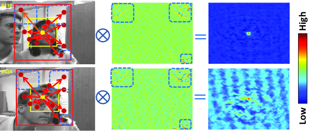
Figure 1: The proposed method handles heavy occlusion well by learning spatio-temporal context information. Note that the region inside the red rectangle is the context region which includes the target and its surrounding background. Left: although the target appearance changes much due to heavy occlusion, the spatial relationship between the object center (denoted by solid yellow circle) and its surrounding locations in the context region (denoted by solid red circles) is almost unchanged. Middle: the learned spatio-temporal context model (the regions inside the blue rectangles have similar values which show the corresponding regions in the left frames have similar spatial relations to the target center.). Right: the learned confidence map.

A generative tracking method learns an appearance model to represent the target and search for image regions with best matching scores as the results. While it is critical to construct an effective appearance model in order to to handle various challenging factors in tracking, the involved computational complexity is often increased at the same time. Furthermore, generative methods discard useful information surrounding target regions that can be exploited to better separate objects from backgrounds. Discriminative methods treat tracking as a binary classification problem with local search which estimates decision boundary between an object image patch and the background. However, the objective of classification is to predict instance labels which is different from the goal of tracking to estimate object locations [16]. Moreover, while some efficient feature extraction techniques (e.g., integral image [14, 15, 16, 17, 18] and random projection [18]) have been proposed for visual tracking, there often exist a large number of samples from which features need to be extracted for classification, thereby entailing computationally expensive operations. Generally speaking, both generative and discriminative tracking algorithms make trade-offs between effectiveness and efficiency of an appearance model. Notwithstanding much progress has been made in recent years, it remains a challenging task to develop an efficient and robust tracking algorithm.

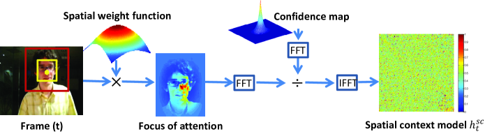
(a) Learn spatial context at the $t$-th frame

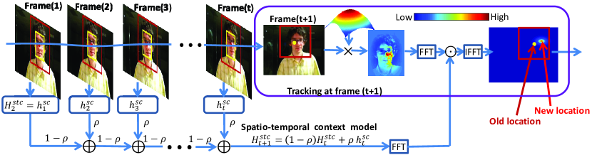
(b) Detect object location at the $(t\rm{+}1)$-th frame

Figure 2: Basic flow of our tracking algorithm. The local context regions are inside the red rectangles while the target locations are indicated by the yellow rectangles. FFT denotes the Fast Fourier Transform and IFFT is the inverse FFT.

In visual tracking, a local context consists of a target object and its immediate surrounding background within a determined region (See the regions inside the red rectangles in Figure 1). Therefore, there exists a strong spatio-temporal relationship between the local scenes containing the object in consecutive frames. For instance, the target in Figure 1 undergoes heavy occlusion which makes the object appearance change significantly. However, the local context containing the object does not change much as the overall appearance remains similar and only a small part of the context region is occluded. Thus, the presence of local context in the current frame helps predict the object location in the next frame. This temporally proximal information in consecutive frames is the temporal context which has been recently applied to object detection [20]. Furthermore, the spatial relation between an object and its local context provides specific information about the configuration of a scene (See middle column in Figure 1) which helps discriminate the target from background when its appearance changes much. Recently, several methods [21, 22, 23, 24] exploit context information to facilitate visual tracking with demonstrated success. However, these approaches require high computational loads for feature extraction in training and tracking phases.

In this paper, we propose a fast and robust tracking algorithm which exploits spatio-temporal local context information. Figure 2 illustrates the basic flow of our algorithm. First, we learn a spatial context model between the target object and its local surrounding background based on their spatial correlations in a scene by solving a deconvolution problem. Next, the learned spatial context model is used to update a spatio-temporal context model for the next frame. Tracking in the next frame is formulated by computing a confidence map as a convolution problem that integrates the spatio-temporal context information, and the best object location can be estimated by maximizing the confidence map (See Figure 2 (b)). Experiments on numerous challenging sequences demonstrate that the proposed algorithm performs favorably against state-of-the-art methods in terms of accuracy, efficiency and robustness.

II Problem Formulation

The tracking problem is formulated by computing a confidence map which estimates the object location likelihood:

$$c(\textbf{x})=P(\textbf{x}|o),$$ (1)

where $\textbf{x}\in\mathbb{R}^{2}$ is an object location and $o$ denotes the object present in the scene. In the following, the spatial context information is used to estimate (17) and Figure 3 shows its graphical model representation.

In the current frame, we have the object location $\textbf{x}^{\star}$ (i.e., coordinate of the tracked object center). The context feature set is defined as $X^{c}=\{\textbf{c}(\textbf{z})=(I(\textbf{z}),\textbf{z})|\textbf{z}\in\Omega_{c}(\textbf{x}^{\star})\}$ where $I(\textbf{z})$ denotes image intensity at location z and $\Omega_{c}(\textbf{x}^{\star})$ is the neighborhood of location $\textbf{x}^{\star}$. By marginalizing the joint probability $P(\textbf{x},\textbf{c}(\textbf{z})|o)$, the object location likelihood function in (17) can be computed by

$$c(\textbf{x}) =P(\textbf{x}|o)$$ (2)

$$=\textstyle\sum_{\textbf{c}(\textbf{z})\in X^{c}}P(\textbf{x},\textbf{c}(\textbf{z})|o)$$

$$=\textstyle\sum_{\textbf{c}(\textbf{z})\in X^{c}}P(\textbf{x}|\textbf{c}(\textbf{z}),o)P(\textbf{c}(\textbf{z})|o),$$

where the conditional probability $P(\textbf{x}|\textbf{c}(\textbf{z}),o)$ models the spatial relationship between the object location and its context information which helps resolve ambiguities when the image measurements allow different interpretations, and $P(\textbf{c}(\textbf{z})|o)$ is a context prior probability which models appearance of the local context. The main task in this work is to learn $P(\textbf{x}|\textbf{c}(\textbf{z}),o)$ as it bridges the gap between object location and its spatial context.

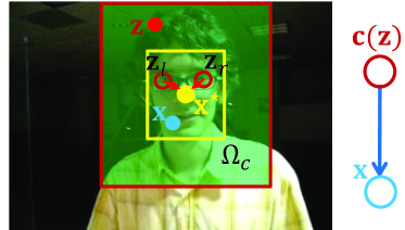
Figure 3: Graphical model representation of spatial relationship between object and its local context. The local context region $\Omega_{c}$ is inside the red rectangle which includes object region surrounding by the yellow rectangle centering at the tracked result $\textbf{x}^{\star}$. The context feature at location z is denoted by $\textbf{c}(\textbf{z})=(I(\textbf{z}),\textbf{z})$ including a low-level appearance representation (i.e., image intensity $I(\textbf{z})$) and location information.

II-A Spatial Context Model

The conditional probability function $P(\textbf{x}|\textbf{c}(\textbf{z}),o)$ in (2) is defined as

$$P(\textbf{x}|\textbf{c}(\textbf{z}),o)=h^{sc}(\textbf{x}-\textbf{z}),$$ (3)

where $h^{sc}(\textbf{x}-\textbf{z})$ is a function (See Section II-D) with respect to the relative distance and direction between object location x and its local context location z, thereby encoding the spatial relationship between an object and its spatial context.

Note that $h^{sc}(\textbf{x}-\textbf{z})$ is not a radially symmetric function (i.e., $h^{sc}(\textbf{x}-\textbf{z})\neq h^{sc}(|\textbf{x}-\textbf{z}|)$), and takes into account different spatial relationships between an object and its local contexts, thereby helping resolve ambiguities when similar objects appear in close proximity. For example, when a method tracks an eye based only on appearance (denoted by $\textbf{z}_{l}$) in the $davidindoor$ sequence shown in Figure 3, the tracker may be easily distracted to the right one (denoted by $\textbf{z}_{r}$) because both eyes and their surrounding backgrounds have similar appearances (when the object moves fast and the search region is large). However, in the proposed method, while the locations of both eyes are at similar distances to location $\textbf{x}^{\star}$ (here, it is location of the context relative to object location $\textbf{z}_{l}$), their relative locations to $\textbf{x}^{\star}$ are different, thereby resulting in different spatial relationships, i.e., $h^{sc}(\textbf{z}_{l}-\textbf{x}^{\star})\neq h^{sc}(\textbf{z}_{r}-\textbf{x}^{\star})$. That is, the non-radially symmetric function $h^{sc}$ helps resolve ambiguities effectively.

II-B Context Prior Model

In (2), the context prior probability is simply modeled by

$$P(\textbf{c}(\textbf{z})|o)=I(\textbf{z})w_{\sigma}(\textbf{z}-\textbf{x}^{\star}),$$ (4)

where $I(\cdot)$ is image intensity that represents appearance of context and $w_{\sigma}(\cdot)$ is a weighted function defined by

$$w_{\sigma}(\textbf{z})=ae^{-\frac{|\textbf{z}|^{2}}{\sigma^{2}}},$$ (5)

where $a$ is a normalization constant that restricts $P(\textbf{c}(\textbf{z})|o)$ in (4) to range from 0 to 1 that satisfies the definition of probability and $\sigma$ is a scale parameter.

In (4), it models focus of attention that is motivated by the biological visual system which concentrates on certain image regions requiring detailed analysis [25]. The closer the context location z is to the currently tracked target location $\textbf{x}^{\star}$, the more important it is to predict the object location in the coming frame, and larger weight should be set. Different from our algorithm that uses a spatially weighted function to indicate the importance of context at different locations, there exist other methods [26, 27] in which spatial sampling techniques are used to focus more detailed contexts at the locations near the object center (i.e., the closer the location is to the object center, the more context locations are sampled).

II-C Confidence Map

The confidence map of an object location is modeled as

$$c(\textbf{x})=P(\textbf{x}|o)=be^{-|\frac{\textbf{x}-\textbf{x}^{\star}}{\alpha}|^{\beta}},$$ (6)

where $b$ is a normalization constant, $\alpha$ is a scale parameter and $\beta$ is a shape parameter (See Figure 4).

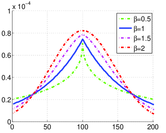
Figure 4: Illustration of 1-D cross section of the confidence map $c$(x) in (6) with different parameters $\beta$. Here, the object location $\textbf{x}^{\star}=(100,100)$.

The object location ambiguity problem often occurs in visual tracking which adversely affects tracking performance. In [17], a multiple instance learning technique is adopted to handle the location ambiguity problem with favorable tracking results. The closer the location is to the currently tracked position, the larger probability that the ambiguity occurs with (e.g., predicted object locations that differ by a few pixels are all plausible solutions and thereby cause ambiguities). In our method, we resolve the location ambiguity problem by choosing a proper shape parameter $\beta$. As illustrated in Figure 4, a large $\beta$ (e.g., $\beta=2$) results in an oversmoothing effect for the confidence value at locations near to the object center, thereby failing to effectively reduce location ambiguities. On the other hand, a small $\beta$ (e.g., $\beta=0.5$) yields a sharp peak near the object center, thereby only activating much fewer positions when learning the spatial context model. This in turn may lead to overfitting in searching for the object location in the coming frame. We find that robust results can be obtained when $\beta=1$ in our experiments.

II-D Fast Learning Spatial Context Model

Based on the confidence map function (6) and the context prior model (4), our objective is to learn the spatial context model (3). Putting (6), (4) and (3) together, we formulate (2) as

$$c(\textbf{x}) =be^{-|\frac{\textbf{x}-\textbf{x}^{\star}}{\alpha}|^{\beta}}$$ (7)

$$=\textstyle\sum_{\textbf{z}\in\Omega_{c}(\textbf{x}^{\star})}h^{sc}(\textbf{x}-\textbf{z})I(\textbf{z})w_{\sigma}(\textbf{z}-\textbf{x}^{\star})$$

$$=h^{sc}(\textbf{x})\otimes(I(\textbf{x})w_{\sigma}(\textbf{x}-\textbf{x}^{\star})),$$

where $\otimes$ denotes the convolution operator.

We note (7) can be transformed to the frequency domain in which the Fast Fourier Transform (FFT) algorithm [28] can be used for fast convolution. That is,

$$\mathcal{F}(be^{-|\frac{\textbf{x}-\textbf{x}^{\star}}{\alpha}|^{\beta}})=\mathcal{F}(h^{sc}(\textbf{x}))\odot\mathcal{F}(I(\textbf{x})w_{\sigma}(\textbf{x}-\textbf{x}^{\star})),$$ (8)

where $\mathcal{F}$ denotes the FFT function and $\odot$ is the element-wise product. Therefore, we have

$$h^{sc}(\textbf{x})=\mathcal{F}^{-1}\bigg{(}\frac{\mathcal{F}(be^{-|\frac{\textbf{x}-\textbf{x}^{\star}}{\alpha}|^{\beta}})}{\mathcal{F}(I(\textbf{x})w_{\sigma}(\textbf{x}-\textbf{x}^{\star}))}\bigg{)},$$ (9)

where $\mathcal{F}^{-1}$ denotes the inverse FFT function.

III Proposed Tracking Algorithm

Figure 2 shows the basic flow of our algorithm. The tracking problem is formulated as a detection task. We assume that the target location in the first frame has been initialized manually or by some object detection algorithms. At the $t$-th frame, we learn the spatial context model $h_{t}^{sc}(\textbf{x})$ (9), which is used to update the spatio-temporal context model $H_{t+1}^{stc}(\textbf{x})$ (12) and applied to detect the object location in the $(t\rm{+}1)$-th frame. When the $(t\rm{+}1)$-th frame arrives, we crop out the local context region $\Omega_{c}(\textbf{x}_{t}^{\star})$ based on the tracked location $\textbf{x}_{t}^{\star}$ at the $t$-th frame and construct the corresponding context feature set $X_{t+1}^{c}=\{\textbf{c}(\textbf{z})=(I_{t+1}(\textbf{z}),\textbf{z})|\textbf{z}\in\Omega_{c}(\textbf{x}_{t}^{\star})\}$. The object location $\textbf{x}_{t+1}^{\star}$ in the $(t\rm{+}1)$-th frame is determined by maximizing the new confidence map

$$\textbf{x}_{t+1}^{\star}=\mathop{\arg\max}_{\textbf{x}\in\Omega_{c}(\textbf{x}_{t}^{\star})}c_{t+1}(\textbf{x}),$$ (10)

where $c_{t+1}(\textbf{x})$ is represented as

$$c_{t+1}(\textbf{x})=\mathcal{F}^{-1}\bigg{(}\mathcal{F}(H_{t+1}^{stc}(\textbf{x}))\odot\mathcal{F}(I_{t+1}(\textbf{x})w_{\sigma_{t}}(\textbf{x}-\textbf{x}_{t}^{\star}))\bigg{)},$$ (11)

which is deduced from (8).

III-A Update of Spatio-Temporal Context

The spatio-temporal context model is updated by

$$H_{t+1}^{stc}=(1-\rho)H_{t}^{stc}+\rho h_{t}^{sc},$$ (12)

where $\rho$ is a learning parameter and $h_{t}^{sc}$ is the spatial context model computed by (9) at the $t$-th frame. We note (12) is a temporal filtering procedure which can be easily observed in frequency domain

$$H_{\omega}^{stc}=F_{\omega}h_{\omega}^{sc},$$ (13)

where $H_{\omega}^{stc}\triangleq\int H_{t}^{stc}e^{-j\omega t}dt$ is the temporal Fourier transform of $H_{t}^{stc}$ and similar to $h_{\omega}^{sc}$. The temporal filter $F_{\omega}$ is formulated as

$$F_{\omega}=\frac{\rho}{e^{j\omega}-(1-\rho)},$$ (14)

where $j$ denotes imaginary unit. It is easy to validate that $F_{\omega}$ in (14) is a low-pass filter [28]. Therefore, our spatio-temporal context model is able to effectively filter out image noise introduced by appearance variations, thereby leading to more stable results.

III-B Update of Scale

According to (11), the target location in the current frame is found by maximizing the confidence map derived from the weighted context region surrounding the previous target location. However, the scale of the target often changes over time. Therefore, the scale parameter $\sigma$ in the weight function $w_{\sigma}$ (5) should be updated accordingly. We propose the scale update scheme as

$$\left\{\begin{array}[]{rl}s_{t}^{\prime}&=\sqrt{\frac{c_{t}(\textbf{x}_{t}^{\star})}{c_{t-1}(\textbf{x}_{t-1}^{\star})}},\\ \overline{s}_{t}&=\frac{1}{n}\sum_{i=1}^{n}s_{t-i}^{\prime},\\ s_{t+1}&=(1-\lambda)s_{t}+\lambda\overline{s}_{t},\\ \sigma_{t+1}&=s_{t}\sigma_{t},\end{array}\right.$$ (15)

where $c_{t}(\cdot)$ is the confidence map that is computed by (11), and $s_{t}^{\prime}$ is the estimated scale between two consecutive frames. To avoid oversensitive adaptation and to reduce noise introduced by estimation error, the estimated target scale $s_{t+1}$ is obtained through filtering in which $\overline{s}_{t}$ is the average of the estimated scales from $n$ consecutive frames, and $\lambda>0$ is a fixed filter parameter (similar to $\rho$ in (12)). The derivation details of (15) can be found in the Appendix Appendex.

III-C Analysis and Discussion

We note that the low computational complexity is one prime characteristic of the proposed algorithm in which only $6$ FFT operations are involved for processing one frame including learning the spatial context model (9) and computing the confidence map (11). The computational complexity for computing each FFT is only $\mathcal{O}(MN\log(MN))$ for the local context region of $M\times N$ pixels, thereby resulting in a fast method ($350$ frames per second in MATLAB on an i$7$ machine). More importantly, the proposed algorithm achieves robust results as discussed bellow.

Difference with related work.

It should be noted that the proposed spatio-temporal context tracking algorithm is significantly different from recently proposed context-based methods [21, 22, 23, 24] and approaches that use FFT for efficient computation [29, 30, 19].

All the above-mentioned context-based methods adopt some strategies to find regions with consistent motion correlations to the object. In [21], a data mining method is used to extract segmented regions surrounding the object as auxiliary objects for collaborative tracking. To find consistent regions, key points surrounding the object are first extracted to help locate the object position [22, 23, 24]. Next, SIFT or SURF descriptors are used to represent these consistent regions [22, 23, 24]. Thus, computationally expensive operations are required in representing and finding consistent regions. Moreover, due to the sparsity nature of key points, some consistent regions that are useful for locating the object position may be discarded. In contrast, the proposed algorithm does not have these problems because all the local regions surrounding the object are considered as the potentially consistent regions, and the motion correlations between the objects and its local contexts in consecutive frames are learned by the spatio-temporal context model that is efficiently computed by FFT.

In [29, 30], the formulations are based on correlation filters that are directly obtained by classic signal processing algorithms. At each frame, correlation filters are trained using a large number of samples, and then combined to find the most correlated position in the next frame. In [19], the filters proposed by [29, 30] are kernelized and used to achieve more stable results. The proposed algorithm is significantly different from [29, 30, 19] in several aspects. First, our algorithm models the spatio-temporal relationships between the object and its local contexts which is motivated by the human visual system that uses context to help resolve ambiguities in complex scenes efficiently and effectively. Second, our algorithm focuses on the regions which require detailed analysis, thereby effectively reducing the adverse effects of background clutters and leading to more robust results. Third, our algorithm handles the object location ambiguity problem using the confidence map with a proper prior distribution, thereby achieving more stable and accurate performance for visual tracking. Finally, our algorithm solves the scale adaptation problem but the other FFT-based tracking methods [29, 30, 19] only track objects with a fixed scale and achieve less accurate results than our method.

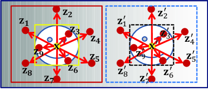
Figure 5: Illustration of why the proposed model is equipped to handle distractor. The target inside the dotted rectangle is the distractor. The different surrounding contexts (e.g., $\textbf{z}_{i}$ and $\textbf{z}_{i}^{\prime}$, $i=1,2,4,5,7,8$) can well discriminate target from distactor.

Robustness to occlusion and distractor.

As shown in Figure 1, the proposed algorithm handles heavy occlusion well as most of context regions are not occluded which have similar relative spatial relations (See middle column of Figure 1) to the target center, thereby helping determine the target center. Figure 5 illustrates our method is robust to distractor (i.e., the right object). If tracking the target only based on its appearance information, the tracker will be distracted to the right one because of their similar appearances. Although the distractor has similar appearance to the target, most of their surrounding contexts have different appearances (See locations $\textbf{z}_{i},\textbf{z}_{i}^{\prime},i=1,2,4,5,7,8$) which are useful to discriminate target from distractor.

IV Experiments

We evaluate the proposed tracking algorithm based on spatio-temporal context (STC) algorithm using $18$ video sequences with challenging factors including heavy occlusion, drastic illumination changes, pose and scale variation, non-rigid deformation, background cluster and motion blur. We compare the proposed STC tracker with $18$ state-of-the-art methods. The parameters of the proposed algorithm are fixed for all the experiments. For other trackers, we use either the original source or binary codes provided in which parameters of each tracker are tuned for best results. The $18$ trackers we compare with are: scale mean-shift (SMS) tracker [2], fragment tracker (Frag) [4], semi-supervised Boosting tracker (SSB) [31], local orderless tracker (LOT) [12], incremental visual tracking (IVT) method [6], online AdaBoost tracker (OAB) [14], multiple instance learning tracker (MIL) [17], visual tracking decomposition method (VTD) [7], L1 tracker (L1T) [9], tracking-learning-detection (TLD) method [15], distribution field tracker (DF) [11], multi-task tracker (MTT) [13], structured output tracker (Struck) [16], context tracker (ConT) [23], minimum output sum of square error (MOS) tracker [30], compressive tracker (CT) [18], circulant structure tracker (CST) [19] and local-global tracker (LGT) [32]. For the trackers involving randomness, we repeat the experiments $10$ times on each sequence and report the averaged results. Implemented in MATLAB, our tracker runs at $350$ frames per second (FPS) on an i$7$ $3.40$ GHz machine with $8$ GB RAM. The MATLAB source codes will be released.

IV-A Experimental Setup

The size of context region is initially set to twice the size of the target object. The parameter $\sigma_{t}$ of (15) is initially set to $\sigma_{1}=\frac{s_{h}+s_{w}}{2}$, where $s_{h}$ and $s_{w}$ are height and width of the initial tracking rectangle, respectively. The parameters of the map function are set to $\alpha=2.25$ and $\beta=1$. The learning parameter $\rho=0.075$. The scale parameter $s_{t}$ is initialized to $s_{1}=1$, and the learning parameter $\lambda=0.25$. The number of frames for updating the scale is set to $n=5$. To reduce effects of illumination change, each intensity value in the context region is normalized by subtracting the average intensity of that region. Then, the intensity in the context region multiplies a Hamming window to reduce the frequency effect of image boundary when using FFT [28, 29].

TABLE I: Success rate (SR)(%). Red fonts indicate the best performance while the blue fonts indicate the second best ones. The total number of evaluated frames is $7,591$.

Sequence	SMS [2]	Frag [4]	SSB [31]	LOT [12]	IVT [6]	OAB [14]	MIL [17]	VTD [7]	L1T [9]	TLD [15]	DF [11]	MTT [13]	Struck [16]	ConT [23]	MOS [30]	CT [18]	CST [19]	LGT [32]	STC
animal	13	3	51	15	4	17	83	96	6	37	6	87	93	58	3	92	94	7	94
bird	33	64	13	5	78	94	10	9	44	42	94	10	48	26	11	8	47	89	65
bolt	58	41	18	89	15	1	92	3	2	1	2	2	8	6	25	94	39	74	98
cliffbar	5	24	24	26	47	66	71	53	24	62	26	55	44	43	6	95	93	81	98
chasing	72	77	62	20	82	71	65	70	72	76	70	95	85	53	61	79	96	95	97
car4	10	34	22	1	97	30	37	35	94	88	26	22	96	90	28	36	44	33	98
car11	1	1	19	32	54	14	48	25	46	67	78	59	18	47	85	36	48	16	86
cokecan	1	3	38	4	3	53	18	7	16	17	13	85	94	20	2	30	86	18	87
downhill	81	89	53	6	87	82	33	98	66	13	94	54	87	71	28	82	72	73	99
dollar	55	41	38	40	21	16	46	39	39	39	100	39	100	100	89	87	100	100	100
davidindoor	6	1	36	20	7	24	30	38	18	96	64	94	71	82	43	46	2	95	100
girl	7	70	49	91	64	68	28	68	56	79	59	71	97	74	3	27	43	51	98
jumping	2	34	81	22	100	82	100	87	13	76	12	100	18	100	6	100	100	5	100
mountainbike	14	13	82	71	100	99	18	100	61	26	35	100	98	25	55	89	100	74	100
ski	22	5	65	55	16	58	33	6	5	36	6	9	76	43	1	60	1	71	68
shaking	2	25	30	14	1	39	83	98	3	15	84	2	48	12	4	84	36	48	96
sylvester	70	34	67	61	45	66	77	33	40	89	33	68	81	84	6	77	84	85	78
woman	52	27	30	16	21	18	21	35	8	31	93	19	96	28	2	19	21	66	100
Average SR	35	35	45	35	49	49	52	49	40	62	53	59	75	62	26	62	60	68	94

TABLE II: Center location error (CLE)(in pixels) and average frame per second (FPS). Red fonts indicate the best performance while the blue fonts indicate the second best ones. The total number of evaluated frames is $7,591$.

Sequence	SMS [2]	Frag [4]	SSB [31]	LOT [12]	IVT [6]	OAB [14]	MIL [17]	VTD [7]	L1T [9]	TLD [15]	DF [11]	MTT [13]	Struck [16]	ConT [23]	MOS [30]	CT [18]	CST [19]	LGT [32]	STC
animal	78	100	25	70	146	62	32	17	122	125	252	17	19	76	281	18	16	166	15
bird	25	13	101	99	13	9	140	57	60	145	12	156	21	139	159	79	20	11	15
bolt	42	43	102	9	65	227	9	177	261	286	277	293	149	126	223	10	210	12	8
cliffbar	41	34	56	36	37	33	13	30	40	70	52	25	46	49	104	6	6	10	5
chasing	13	9	44	32	6	9	13	23	9	47	31	5	6	16	68	10	5	6	4
car4	144	56	104	177	14	109	63	127	16	13	92	158	9	11	117	63	44	47	11
car11	86	117	11	30	7	11	8	20	8	12	6	8	9	8	8	9	8	16	7
cokecan	60	70	15	46	64	11	18	68	40	29	30	10	7	36	53	16	9	32	6
downhill	14	11	102	226	22	12	117	9	35	255	10	77	10	62	116	12	129	12	8
dollar	55	56	66	66	23	28	23	65	65	72	3	71	18	5	12	20	5	4	2
davidindoor	176	103	45	100	281	43	33	40	86	13	27	11	20	22	78	28	149	12	8
girl	130	26	50	12	36	22	34	41	51	23	27	23	8	34	126	39	43	35	9
jumping	63	30	11	43	4	11	4	17	45	13	73	7	42	4	155	6	3	89	4
mountainbike	135	209	11	24	5	11	208	7	74	213	155	7	8	149	16	11	5	12	6
ski	91	134	10	12	51	11	15	179	161	222	147	33	8	78	386	11	237	13	12
shaking	224	55	133	90	134	22	11	5	72	232	11	115	23	191	194	11	21	33	10
sylvester	15	47	14	23	138	12	9	66	49	8	56	18	9	13	65	9	7	11	11
woman	49	118	86	131	112	120	119	110	148	108	12	169	4	55	176	122	160	23	5
Average CLE	79	63	54	70	84	43	43	58	62	78	52	80	19	42	103	29	54	22	8
Average FPS	12	7	11	0.7	33	22	38	5	1	28	13	1	20	15	200	90	120	8	350

IV-B Experimental Results

We use two evaluation criteria to quantitatively evaluate the $19$ trackers: the center location error (CLE) and success rate (SR), both computed based on the manually labeled ground truth results of each frame. The score of success rate is defined as $score=\frac{area(R_{t}\bigcap R_{g})}{area(R_{t}\bigcup R_{g})}$, where $R_{t}$ is a tracked bounding box and $R_{g}$ is the ground truth bounding box, and the result of one frame is considered as a success if $score>0.5$. Table I and Table II show the quantitative results in which the proposed STC tracker achieves the best or second best performance in most sequences both in terms of center location error and success rate. Furthermore, the proposed tracker is the most efficient ($350$ FPS on average) algorithm among all evaluated methods. Although the CST [19] and MOS [30] methods also use FFT for fast computation, the CST method performs time-consuming kernel operations and the MOS tracker computes several correlation filters in each frame, thereby making these two approaches less efficient than the proposed algorithm. Furthermore, both CST and MOS methods only track target with fixed scale, which achieve less accurate results that the proposed method with scale adaptation. Figure 6 shows some tracking results of different trackers. For presentation clarity, we only show the results of the top $7$ trackers in terms of average success rates.

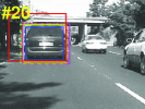
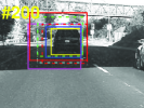
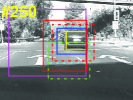
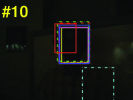
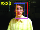
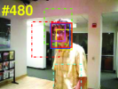
(a) car4	(b) davidindoor
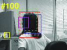
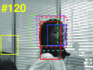
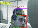
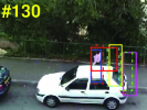
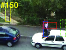
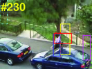
(c) girl	(d) woman
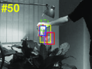
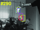
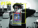
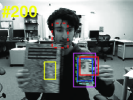
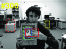
(e) cokecan	(f) cliffbar

Figure 6: Screenshots of tracking results.

Illumination, scale and pose variation.

There are large illumination variations in the evaluated sequences. The appearance of the target object in the car4 sequence changes significantly due to the cast shadows and ambient lights (See $\#200,\#250$ in the car4 sequence shown in Figure 6). Only the models of the IVT, L1T, Struck and STC methods adapt to these illumination variations well. Likewise, only the VTD and our STC methods perform favorably on the shaking sequence because the object appearance changes drastically due to the stage lights and sudden pose variations. The davidindoor sequence contain gradual pose and scale variations as well as illumination changes. Note that most reported results using this sequence are only on subsets of the available frames, i.e., not from the very beginning of the davidindoor video when the target face is in nearly complete darkness. In this work, the full sequence is used to better evaluate the performance of all algorithms. Only the proposed algorithm is able to achieve favorable tracking results on this sequence both in terms of accuracy and success rate. This can be attributed to the use of spatio-temporal context information which facilitates filtering out noisy observations (as discussed in Section III-A), thereby enabling the proposed STC algorithm to relocate the target when object appearance changes drastically due to illumination, scale and pose variations.

Occlusion, rotation, and pose variation.

The target objects in the woman, girl and bird sequences are partially occluded at times. The object in the girl sequence also undergoes in-plane rotation (See $\#100,\#120$ of the girl sequence in Figure 6) which makes the tracking tasks difficult. Only the proposed algorithm is able to track the objects successfully in most frames of this sequence. The woman sequence has non-rigid deformation and heavy occlusion (See $\#130,\#150,\#230$ of the woman sequence in Figure 6) at the same time. All the other trackers fail to successfully track the object except the Struck and the proposed STC algorithms. As most of the local contexts surrounding the target objects are not occluded in these sequences, such information facilitates the proposed algorithm relocating the object even they are almost fully occluded (as discussed in Figure 1).

Background clutter and abrupt motion.

In the animal, cokecan and cliffbar sequences, the target objects undergo fast movements in the cluttered backgrounds. The target object in the chasing sequence undergoes abrupt motion with 360 degree out-of-plane rotation, and the proposed algorithm achieves the best performance both in terms of success rate and center location error. The cokecan video contains a specular object with in-plane rotation and heavy occlusion, which makes this tracking task difficult. Only the Struck and the proposed STC methods are able to successfully track most of the frames. In the cliffbar sequence, the texture in the background is very similar to that of the target object. Most trackers drift to background except the CT, CST, LGT and our methods (See $\#300$ of the cliffbar sequence in Figure 6). Although the target and its local background have very similar texture, their spatial relationships and appearances of local contexts are different which are used by the proposed algorithm when learning a confidence map (as discussed in Section III-C). Hence, the proposed STC algorithm is able to separate the target object from the background based on the spatio-temporal context.

V Conclusion

In this paper, we present a simple yet fast and robust algorithm which exploits spatio-temporal context information for visual tracking. Two local context models (i.e., spatial context and spatio-temporal context models) are proposed which are robust to appearance variations introduced by occlusion, illumination changes, and pose variations. The Fast Fourier Transform algorithm is used in both online learning and detection, thereby resulting in an efficient tracking method that runs at $350$ frames per second with MATLAB implementation. Numerous experiments with state-of-the-art algorithms on challenging sequences demonstrate that the proposed algorithm achieves favorable results in terms of accuracy, robustness, and speed.

Appendex

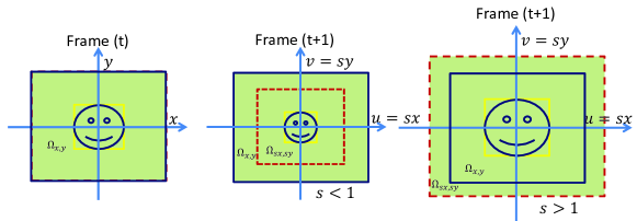
Figure 7: Illustration of scale change. From left to right, the scale ratio is $s$. $\Omega_{x,y}$ inside the solid rectangles denotes the context region at the $t$-th frame, and its corresponding context region at the ($t+1$)-th frame is denoted by $\Omega_{sx,sy}$ that is inside the dotted rectangles.

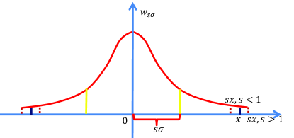
Figure 8: Illustration of 1-D cross section of the weight function $w_{s\sigma}(\textbf{x})$.

Without loss of generality, we assume the target object is centered at $\textbf{x}^{\star}=(0,0)$. Then, the confidence map (i.e., (11)) can be represented as

$$c(\textbf{x})=H(\textbf{x})\otimes(I(\textbf{x})w_{\sigma}(\textbf{x})).$$ (16)

Then, we have

$$c(0,0)=\int\int_{\Omega_{x,y}}H(x,y)I(-x,-y)w_{\sigma}(-x,-y)dxdy.$$ (17)

See Figure 7, when size of the target changes from left to right with ratio $s$, performing a change of variables $(u,v)=(sx,sy)$, we can reformulate (17)

$$c_{t}(0,0) =\int\int_{\Omega_{x,y}}H_{t}(x,y)I_{t}(-x,-y)w_{\sigma_{t}}(-x,-y)dxdy$$ (18)

$$=\int\int_{\Omega_{sx,sy}}H_{t}(u/s,v/s)I_{t}(-u/s,-v/s)w_{\sigma_{t}}(-u/s,-v/s)\frac{1}{s^{2}}dudv$$

$$=\int\int_{\Omega_{sx,sy}}H_{t}(u/s,v/s)I_{t+1}(-u,-v)w_{\sigma_{t}}(-u/s,-v/s)\frac{1}{s^{2}}dudv$$

$$=\int\int_{\Omega_{sx,sy}}H_{t}(u/s,v/s)w_{s\sigma_{t}}(-u,-v)I_{t+1}(-u,-v)\frac{1}{s^{2}}dudv$$

$$\approx\int\int_{\Omega_{sx,sy}}H_{t+1}(u,v)w_{s\sigma_{t}}(-u,-v)I_{t+1}(-u,-v)\frac{1}{s^{2}}dudv$$

$$=\int\int_{\Omega_{x,y}}H_{t+1}(u,v)w_{s\sigma_{t}}(-u,-v)I_{t+1}(-u,-v)\frac{1}{s^{2}}dudv-\underbrace{\int\int_{\Omega_{x,y}\backslash\Omega_{sx,sy}}H_{t+1}(u,v)w_{s\sigma_{t}}(u,v)I_{t+1}(-u,-v)\frac{1}{s^{2}}dudv}_{\approx 0\ \textrm{because}\ w_{s\sigma_{t}}(-u,-v)\approx 0\ \textrm{for}\ \textrm{all}\ (u,v)\in\Omega_{x,y}\backslash\Omega_{sx,sy}(\mathrm{See~{}Figure}~{}\ref{fig:scaleweight})}$$

$$\approx\int\int_{\Omega_{x,y}}H_{t+1}(u,v)w_{s\sigma_{t}}(-u,-v)I_{t+1}(-u,-v)\frac{1}{s^{2}}dudv.$$

In (LABEL:eq:scale), we have used the following relationships

$$H_{t}(u/s,v/s)\approx H_{t+1}(u,v),$$ (19)

$$I_{t}(u/s,v/s)\approx I_{t+1}(u,v).\\$$ (20)

Because of the proximity between two consecutive frames, as in [2], we can make the above reasonable assumptions which are spatially scaled versions of $I_{t}$ and $H_{t}$, respectively.

It is difficult to estimate $s$ from the (LABEL:eq:scale) because of the nonlinearity of the Gaussian weight function $w_{s\sigma_{t}}$. We adopt an iterative method to approximately obtain $s$. We utilize the estimated scale $s_{t}$ at frame $t$ to replace the scale term $s$ in the Gaussian window $w_{s\sigma_{t}}$, and the other scale term that needs to estimate is denoted as $s_{t+1}$. Thus, (LABEL:eq:scale) is reformulated as

$$c_{t}(0,0) \approx\int\int_{\Omega_{x,y}}H_{t+1}(u,v)w_{s_{t}\sigma_{t}}(-u,-v)I_{t+1}(-u,-v)\frac{1}{s_{t+1}^{2}}dudv$$ (21)

$$=\int\int_{\Omega_{x,y}}H_{t+1}(u,v)w_{\sigma_{t+1}}(-u,-v)I_{t+1}(-u,-v)\frac{1}{s_{t+1}^{2}}dudv$$

$$=\frac{1}{s_{t+1}^{2}}c_{t+1}(0,0),$$

where we denote

$$\sigma_{t+1}=s_{t}\sigma_{t}.$$ (22)

Thus, we have

$$s_{t+1}=\sqrt{\frac{c_{t+1}(0,0)}{c_{t}(0,0)}}.$$ (23)

We average the scales estimated from the former $n$ consecutive frames to make the current estimation more stable

$$\overline{s}_{t}=\frac{1}{n}\sum_{i=1}^{n}s_{t-i}=\frac{1}{n}\sum_{i=1}^{n}\sqrt{\frac{c_{t-i}(0,0)}{c_{t-i-1}(0,0)}}.$$ (24)

To avoid oversenstive scale adaptation, we utilize the follow equation to incrementally update the estimated scale

$$s_{t+1}=(1-\lambda)s_{t}+\lambda\overline{s}_{t}.$$ (25)

References

- [1] A. Yilmaz, O. Javed, and M. Shah, “Object tracking: A survey,” ACM Computing Surveys, vol. 38, no. 4, 2006.
- [2] R. T. Collins, “Mean-shift blob tracking through scale space,” in CVPR, vol. 2, pp. II–234, 2003.
- [3] R. T. Collins, Y. Liu, and M. Leordeanu, “Online selection of discriminative tracking features,” PAMI, vol. 27, no. 10, pp. 1631–1643, 2005.
- [4] A. Adam, E. Rivlin, and I. Shimshoni, “Robust fragments-based tracking using the integral histogram,” in CVPR, pp. 798–805, 2006.
- [5] M. Yang, J. Yuan, and Y. Wu, “Spatial selection for attentional visual tracking,” in CVPR, pp. 1–8, 2007.
- [6] D. Ross, J. Lim, R. Lin, and M.-H. Yang, “Incremental learning for robust visual tracking,” IJCV, vol. 77, no. 1, pp. 125–141, 2008.
- [7] J. Kwon and K. M. Lee, “Visual tracking decomposition.,” in CVPR, pp. 1269–1276, 2010.
- [8] J. Kwon and K. M. Lee, “Tracking by sampling trackers,” in ICCV, pp. 1195–1202, 2011.
- [9] X. Mei and H. Ling, “Robust visual tracking and vehicle classification via sparse representation,” PAMI, vol. 33, no. 11, pp. 2259–2272, 2011.
- [10] H. Li, C. Shen, and Q. Shi, “Real-time visual tracking using compressive sensing,” in CVPR, pp. 1305–1312, 2011.
- [11] L. Sevilla-Lara and E. Learned-Miller, “Distribution fields for tracking,” in CVPR, pp. 1910–1917, 2012.
- [12] S. Oron, A. Bar-Hillel, D. Levi, and S. Avidan, “Locally orderless tracking,” in CVPR, pp. 1940–1947, 2012.
- [13] T. Zhang, B. Ghanem, S. Liu, and N. Ahuja, “Robust visual tracking via multi-task sparse learning,” in CVPR, pp. 2042–2049, 2012.
- [14] H. Grabner, M. Grabner, and H. Bischof, “Real-time tracking via on-line boosting,” in BMVC, pp. 47–56, 2006.
- [15] Z. Kalal, J. Matas, and K. Mikolajczyk, “Pn learning: Bootstrapping binary classifiers by structural constraints,” in CVPR, pp. 49–56, 2010.
- [16] S. Hare, A. Saffari, and P. H. Torr, “Struck: Structured output tracking with kernels,” in ICCV, pp. 263–270, 2011.
- [17] B. Babenko, M.-H. Yang, and S. Belongie, “Robust object tracking with online multiple instance learning,” PAMI, vol. 33, no. 8, pp. 1619–1632, 2011.
- [18] K. Zhang, L. Zhang, and M.-H. Yang, “Real-time compressive tracking,” in ECCV, pp. 864–877, 2012.
- [19] J. Henriques, R. Caseiro, P. Martins, and J. Batista, “Exploiting the circulant structure of tracking-by-detection with kernels,” in ECCV, pp. 702–715, 2012.
- [20] S. K. Divvala, D. Hoiem, J. H. Hays, A. A. Efros, and M. Hebert, “An empirical study of context in object detection,” in CVPR, pp. 1271–1278, 2009.
- [21] M. Yang, Y. Wu, and G. Hua, “Context-aware visual tracking,” PAMI, vol. 31, no. 7, pp. 1195–1209, 2009.
- [22] H. Grabner, J. Matas, L. Van Gool, and P. Cattin, “Tracking the invisible: Learning where the object might be,” in CVPR, pp. 1285–1292, 2010.
- [23] T. B. Dinh, N. Vo, and G. Medioni, “Context tracker: Exploring supporters and distracters in unconstrained environments,” in CVPR, pp. 1177–1184, 2011.
- [24] L. Wen, Z. Cai, Z. Lei, D. Yi, and S. Li, “online spatio-temporal structure context learning for visual tracking,” in ECCV, pp. 716–729, 2012.
- [25] A. Torralba, “Contextual priming for object detection,” IJCV, vol. 53, no. 2, pp. 169–191, 2003.
- [26] S. Belongie, J. Malik, and J. Puzicha, “Shape matching and object recognition using shape contexts,” PAMI, vol. 24, no. 4, pp. 509–522, 2002.
- [27] L. Wolf and S. Bileschi, “A critical view of context,” IJCV, vol. 69, no. 2, pp. 251–261, 2006.
- [28] A. V. Oppenheim, A. S. Willsky, and S. H. Nawab, Signals and systems, vol. 2. Prentice-Hall Englewood Cliffs, NJ, 1983.
- [29] D. S. Bolme, B. A. Draper, and J. R. Beveridge, “Average of synthetic exact filters,” in CVPR, pp. 2105–2112, 2009.
- [30] D. S. Bolme, J. R. Beveridge, B. A. Draper, and Y. M. Lui, “Visual object tracking using adaptive correlation filters,” in CVPR, pp. 2544–2550, 2010.
- [31] H. Grabner, C. Leistner, and H. Bischof, “Semi-supervised on-line boosting for robust tracking,” in ECCV, pp. 234–247, 2008.
- [32] L. Cehovin, M. Kristan, and A. Leonardis, “Robust visual tracking using an adaptive coupled-layer visual model,” PAMI, vol. 35, no. 4, pp. 941–953, 2013.