ELM processes and properties in 2T 2MA ITER-like wall JET plasmas

Abstract

During July 2012, 150 almost identical H-mode plasmas were consecutively created in the Joint European Torus (JET), providing a combined total of approximately 8 minutes of steady-state plasma with 15,000 Edge Localised Modes (ELMs). In principle, each of those 15,000 ELMs are statistically equivalent. Here the changes in edge density and plasma energy associated with those ELMs are explored, using the spikes in Beryllium II (527 nm) radiation as an indicator for the onset of an ELM. Clearly different timescales are observed during the ELM process. Edge temperature falls over a 2ms timescale, edge density and pressure fall over a 5ms timescale, and there is an additional 10ms timescale that is consistent with a resistive relaxation of the plasma’s edge. The statistical properties of the energy and density losses due to the ELMs are explored. For these plasmas the ELM energy ($\delta E$) is found to be approximately independent of the time between ELMs, despite the average ELM energy ($\langle E\rangle$) and average ELM frequency ($f$) being consistent with the scaling of $\langle\delta E\rangle\propto 1/f$. Instead, beyond the first 0.02 seconds of waiting time between ELMs, the energy losses due to individual ELMs are found to be statistically the same. Surprisingly no correlation is found between the energies of consecutive ELMs either. A weak link is found between the density drop and the ELM waiting time. Consequences of these results for ELM control and modelling are discussed.

I Introduction

Edge Localised Modes (ELMs) are instabilities that occur at the edge of tokamak plasmas Wesson . They are thought to be triggered by an ideal Magnetohydrodynamic (MHD) instability of the plasma’s edge EPED1 ; WebsterNF , and are presently found in nearly all high confinement tokamak plasmas Keilhacker84 ; Zohm ; Kamiya . Large ELMs such as those that are predicted to occur in ITER Aymar ; Lipschultz ; Loarte , will need to be reduced in size or avoided entirely if plasma-facing components are to have a reasonable lifetime. One way to reduce ELM size is by “pacing” the ELMs at higher frequencies than their natural rate of occurrence Liang ; LangPacing , because they are expected to occur with a lower energy due to the empirically observed relationship between ELM energy ($\delta E$) and ELM frequency ($f$) of $\delta E\propto 1/f$ Hermann . The ELM frequency is usually reported as an average over all ELMs in a given pulse, and is identical to one divided by the average waiting time between the ELMs. In contrast to the relationships between the average ELM energy and average ELM frequency, the relationship between an individual ELM’s energy and its individual “frequency” (often defined as one divided by its waiting time since the previous ELM), is rarely reported. It is this topic that is considered here.

Since 2011 the JET tokamak has been operating with its previously Carbon plasma-facing components replaced with the metal ITER-like wall Rudi . This has led to differences in plasma confinement and ELM properties, as discussed for example in Rudi ; Maddison and references therein. This paper focuses its attention on a set of 150 JET plasmas produced over a two week period in July 2012, 120 of which were nearly identical, providing $\sim$10,000 statistically equivalent ELMs. Such high quality statistical information on ELM properties has never previously been available. The pulses are 2 Tesla 2 Mega Amp H-mode plasmas with approximately 12MW of NBI heating, a fuelling rate of 1.4$\times 10^{22}$ Ds^-1, Z_eff=1.2, and a triangularity of $\delta$=0.2, see NewRef2 for further details, including a large selection of time traces. The plasmas each have approximately 6 seconds of steady H-mode, 2.3 seconds of which between 11.5 and 13.8 seconds is exceptionally steady and is what we consider here and in previous work EPSResonances ; Resonances .

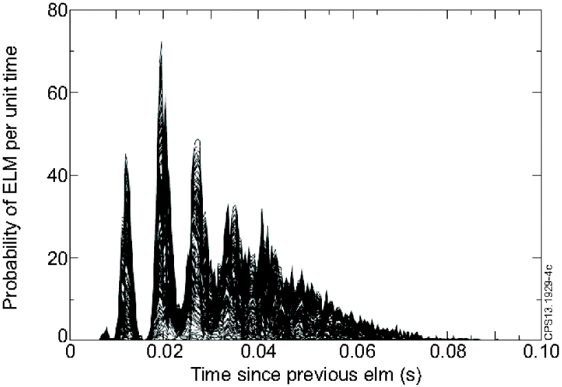
Figure 1: The probability density function (pdf) for the waiting time between ELM events, determined from the ELM waiting time data from 120 equivalent pulses (see text for details). Each line corresponds to data from an individual pulse. Reproduced from Ref. Resonances .

The large quantities of extremely high quality steady-state data that these plasmas provide, allows statistical methods to observe details that could not otherwise be seen, such as an unexpected series of maxima and minima in the probability density function (pdf) for the waiting times between ELMs that was created from the experimental data (see figure 1, reproduced from Ref. Resonances ). The series of maxima and minima in figure 1 are not due to different ELM frequencies in different pulses, but arise from a sequence of statistically almost independent ELM events, whose resulting probability distribution is in figure 1. The cause of this phenomenon is not fully understood, and is presently under investigation, preliminary results are in Refs. EPSResonances and Resonances . A question that motivated this paper was whether the maxima and minima in figure 1 had a similar distribution of ”quantised” ELM energies. The answer we will find is no, but the excellent statistical information has led to a number of other surprising results that we will report here. It is worth noting that it requires of order 250-500 ELMs to clearly observe the 4-5 maxima and minima of figure 1. This typically will require pulses to be repeated 4-5 times, and considerably more if we are to ensure that the statistical noise is kept small. It also requires pulses that are extremely steady. Such large quantities of high quality data are not generally available, and as a result, it is not possible at present to be certain about how common the phenomenon is, or whether it is only present in ITER-like wall plasmas. We will find no evidence that the phenomenon is affecting the ELM energies at all, it seems solely to affect the times at which ELMs are triggered. Therefore the phenomenon is not discussed further here, but seems likely to be important for understanding how ELMs are triggered.

The outline of the paper is as follows. In Section II we describe how we determine and define individual ELM sizes. In Section III we describe the statistical properties of the ELMs. Section IV considers the average evolution of the edge temperature and pressure, and in Section V we discuss the results and propose our conclusions.

II Defining the energy and density drop due to an ELM

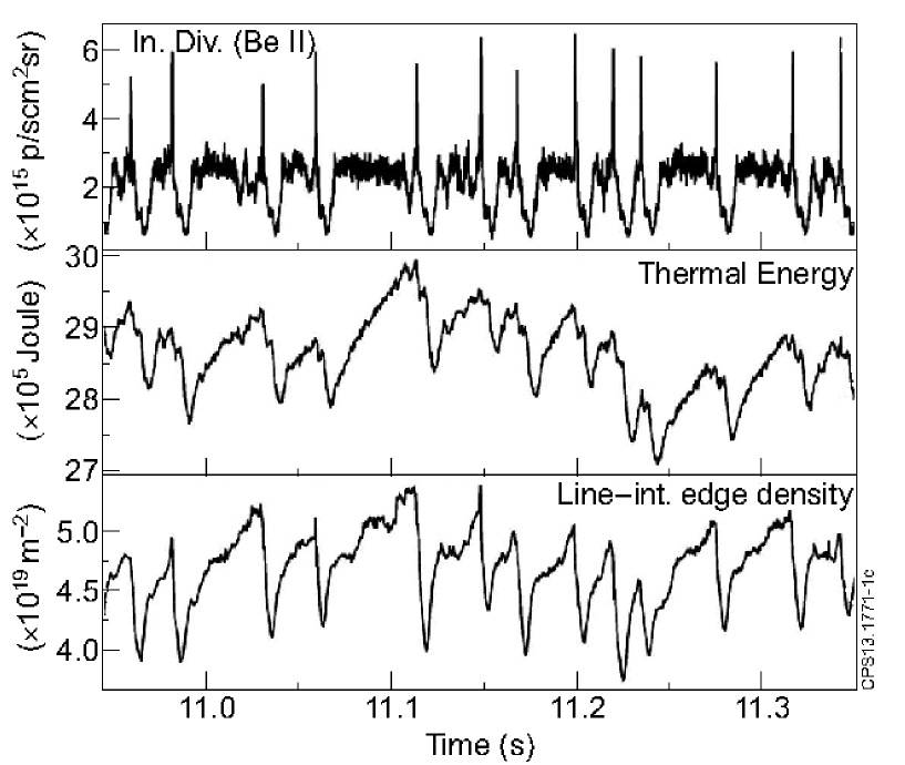
Figure 2: From top to bottom: i) The Be II (527nm) signal measured at the inner divertor, that is used to identify ELMs from the sharp spikes in radiation. ii) The estimated thermal energy stored in the plasma, which is calculated by EFIT using magnetic measurements to reconstruct the MHD equilibrium and infer the plasma’s pressure. The thermal energy is $3/2$ times the volume integral of the plasma pressure, sometimes referred to as the plasma’s “kinetic” energy. iii) The line-integrated plasma number density at the plasma’s edge. For each ELM there is a sharp spike in Be II emission, shortly followed by a drop in density to a minimum at around 0.005s after the ELM started, and a drop in the plasma’s thermal energy to a minimum some time around 0.01s after the ELM started.

The main purpose of this paper is to explore the relationship between the losses of plasma energy or density due to ELMs, and the waiting times between the ELMs. The signals that are used are the line integrated edge plasma density, which is a direct line-integrated measure of the density at the plasma’s edge, and the plasma’s thermal energy as inferred from a collection of magnetic diagnostics using EFIT EFIT ; EFIT2 , both of which are checked and compared with independent Thompson scattering measurements. The Beryllium II (527nm) radiation that is measured at the inner divertor is used to determine when ELMs occur, using the method described in WebsterDendyPRL , that detects the statistically large spikes in radiation that are associated with ELMs. For the type I ELMs in the H-mode plasmas considered here, the ELMs are easy to identify with this method. All the signals just described are standard and widely used JET signals. An advantage of the signals chosen is that they are independent measurements for: the line integrated density, the Be II light emissions, and the thermal energy losses inferred from magnetic measurements; and the former two measurements are direct measurements requiring minimal reconstruction from diagnostic data. Following an ELM there is a small radial plasma motion by 7-8mm, that in principle can affect measurements. Appendix A confirms that for the plasmas studied here at least, this can be neglected in comparison to the much larger changes in the post-ELM measurements. Next we will firstly discuss the measured changes to the line integrated plasma density, we will find that similar remarks apply to changes in the plasma’s energy.

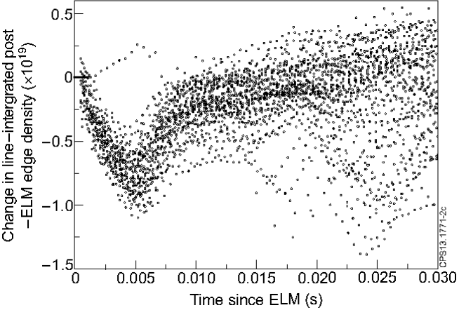
Figure 3: The fall in line-integrated edge density with time since each ELM is plotted for a typical pulse in the set (pulse number 83790). There is a clearly visible minima at around 0.005 seconds. Beyond about 0.012 seconds there are a small number of additional drops in density due to ELMs that occur within the 0.03 second time interval that is plotted.

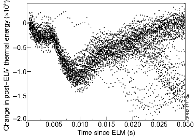
Figure 4: The fall in the plasma’s thermal energy with time since each ELM is plotted for a typical pulse in the set (pulse number 83790). There are two clearly visible minima, one between 0.002 and 0.005 seconds, and another at around 0.01 seconds. Beyond about 0.012 seconds there are a small number of additional drops in energy due to ELMs that occur within the 0.03 second time interval that is plotted.

Following an ELM, the line integrated plasma density falls, then recovers again (see figure 2). The losses associated with the ELM have a duration of order 0.005 seconds, that combined with fluctuations in the signal can make it difficult to define the density loss due to the ELM. For example, figure 3 shows the fall in edge density with time since an ELM for ELMs in the typical pulse 83790. There is clearly a minimum in the line integrated signal at around 0.005 seconds, or in equivalent words, there is a maximum drop in line integrated edge density at around 0.005 seconds. The exact time and magnitude of the minimum is not always the same. Here we define the density drop due to an ELM ($\delta n$) as the maximum observed drop in the line-integrated density within a small time interval $t_{m}$ after an ELM (see figure 5). Note that figures 2, 3, and 4 discuss time traces in which there are minima in line-integrated density or thermal energy after an ELM, whereas from figure 5 onwards we consider the maximum energy and density lost after an ELM, which is a positive quantity. Figure 5 shows that if $\delta n$ is defined in this way then provided $t_{m}$ is greater than about 0.005 seconds, which is much less than the 0.012 second waiting time to the most frequent ELMs EPSResonances ; Resonances , then $\delta n$ is independent of $t_{m}$. Consequently provided $t_{m}$ is greater than 0.005 seconds, then $\delta n$ is independent of $t_{m}$ and is well defined. For plots involving drops in edge density we use $t_{m}=$ 0.01 seconds, and for plots involving drops in energy we will specify whether we are discussing results with $t_{m}=$ 0.01 or $t_{m}=$0.005 seconds.

Similar remarks apply to the plasma’s thermal energy, which is defined as $3/2$ times the volume integral of the plasma’s pressure, with the pressure here obtained from an ideal MHD reconstruction of the equilibrium using EFIT EFIT ; EFIT2 . The thermal energy is sometimes referred to as “kinetic energy”, but does not include the energy due to macroscopic flows in the plasma. The drop in thermal energy ($\delta E$) is defined as the minimum energy in some time period $t_{m}$ immediately following an ELM. A difference is that there are now two timescales that can clearly be observed (see figures 4 and 6). The first minimum in energy occurs between 0.002 and 0.005 seconds, which tends to be before the minima at 0.005s found in figure 5. However, unlike the density, there is a second minimum at around 0.01 seconds (see figure 4). The possible causes of the different timescales are discussed in greater detail later. Beyond 0.01 seconds the average of $\delta E$ is approximately independent of $t_{m}$, allowing $\delta E$ to be defined as either the minimum thermal energy in the time interval between an ELM and $t_{m}=0.005$ seconds or between an ELM and $t_{m}$=0.01 seconds (see figure 6). Both of these are less than the time of the first maxima in the ELM waiting time distribution EPSResonances ; Resonances , that is at approximately 0.012 seconds. This suggests two possible definitions for the ELM energy, as either the maximum energy lost over the 0.005 second timescale during which particle loss is also leading to a reduction in the edge density (see figures 5 and 6), or as the total reduction in stored thermal energy over 0.01 seconds. Both will be reported and discussed here, and both can be observed in the time traces in figure 2, with a small minimum in $\delta E$ prior to the minimum in the density, followed by a much larger minimum in $\delta E$ on the larger timescale of $\sim 0.01$ seconds.

Two timescales have previously been reported in conjunction with the edge electron temperature during the post-ELM pedestal recovery in ITER-like wall plasmas Beurskens ; Frassinetti , an important difference is that here the two timescales are observed with every ELM. It is possible that the two timescales relate to a similar sequence of processes - rapid energy losses followed by slower transport processes. The timescale for the initial fall in edge temperature reported in Refs. Beurskens ; Frassinetti is only about 0.002 seconds, whereas the drop in edge density (figures 3 and 5), is over a 0.005 second timescale. Two timescales have also been reported in conjunction with infra red (IR) images of JET’s divertor during Carbon-wall JET experiments Eich1 . In this latter work the two timescales arose from the shape of the ELM power deposition curve with respect to time, and are much shorter than those discussed so far. The timescales characterise the initial rapid rise in ELM power deposition, over a timescale time $\tau_{rise}\sim 0.0002-0.0005$ seconds, and a slower $\tau_{decay}\sim 0.001-0.0025$ seconds that characterises the subsequent fall in the power deposition.

The work referred to above and the results here are consistent with, and possibly extend, the proposed sequence of steps by which energy is lost during an ELM Loarte . Firstly there is a rapid rise in heat flux that for Carbon-wall plasmas was found over a timescale of order 0.2-0.5 milliseconds Eich1 , with heat being lost predominately by electrons. In ITER-like wall plasmas, after of order 1-2 milliseconds the edge temperature is found to fall to a minimum Beurskens ; Frassinetti , something we find here also in Section IV. This process of energy loss is referred to as “conduction” Loarte . Next, for the plasmas described here at least, there is a loss of ions that is completed within a timescale of order 5 milliseconds (figure 5), in a process referred to as “convection” Loarte . Finally we find an additional timescale of order 10 milliseconds after an ELM (figure 6), during which EFIT EFIT ; EFIT2 suggests that the thermal plasma energy relaxes to a minimum, before starting to rise again. As discussed in Section IV, EFIT’s reconstructed measurements are consistent with direct Thompson scattering measurements over the 0-5 millisecond time period, but disagree between 5-10 milliseconds when EFIT suggests that the thermal energy continues to fall. Appendix B explores the timescales associated with a resistive relaxation of the pedestal at the plasma’s edge Frassinetti2 , and finds a timescale of 8 milliseconds, very similar to the 10 millisecond timescale observed in figures 4 and 6. Consequently it is possible that a resistive mechanism is allowing the plasma to relax to a new post-ELM equilibrium, and that one or more non-ideal affects are making EFIT’s ideal-MHD equilibrium reconstruction unreliable over this longer time period. Similarly, resistive effects can only become important over timescales approaching 8 milliseconds, which may explain why EFIT’s calculated pressure agrees with that measured by Thompson scattering over the shorter 0-5 millisecond timescale (see Section IV). It is interesting to note that 8 milliseconds is the approximate time between the maxima and minima observed in the ELM waiting time pdf in figure 1 EPSResonances ; Resonances , that will be observed later in the time periods between the clusters of ELMs in figures 7, 8, and 9. We do not know whether this is a coincidence or not.

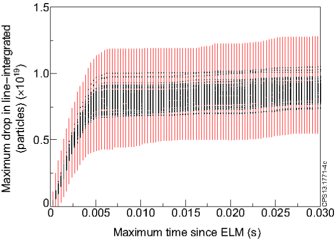
Figure 5: The maximum drop in line integrated plasma density ($\delta n$) following an ELM (vertical axis), is plotted against the (maximum) time $t_{m}$ since the ELM (horizontal axis), over which the maximum drop is calculated. For each plasma $\delta n$ is averaged over all the ELMs in a given pulse (plotted points), and its standard deviation calculated (vertical lines). This is repeated for each maximum time $t_{m}$ since the ELM, and for each plasma pulse. There is a comparatively small scatter of about 15-20% between the average value’s of $\delta n$ for the 120 different pulses, confirming that the pulses are quite similar. Consequently if $t_{m}$ is taken to be greater than about 0.005 seconds then there is a well defined $\delta n$ that is independent of $t_{m}$. The timescale of 0.005 seconds is much less than the time between ELMs.

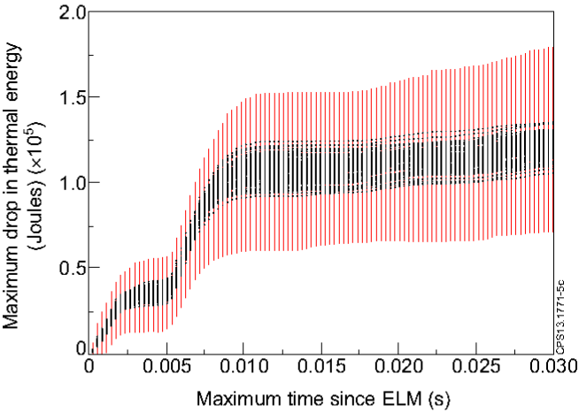
Figure 6: For $t_{m}$ from 0 to 0.03 seconds and for all 120 pulses, the minimum thermal energy within time $t_{m}$ after an ELM is averaged over all ELMs in a pulse (plotted points), and the standard deviation about this average is calculated also (vertical lines). The 120 sets of averages (plotted points) and standard deviations (red lines) have been plotted over one another so as to present them on a single graph. Two time scales are evident. The first at 0.005 seconds is the same as found in figure 5. The second timescale is at 0.01 seconds, beyond which the average value of $\delta E$ is approximately constant, independent of $t_{m}$.

III Statistical properties of ELMs

Next we look at how these measures of the density and energy losses associated with the ELMs are influenced by the waiting times between the ELMs (see figures 7, 8, and 9). The most obvious characteristic of both figures is the vertical clustering of ELM times. This is due to the waiting-time probability density function (pdf) in figure 1, which is discussed in detail in Refs. EPSResonances ; Resonances , and shows a series of maxima and zeros at approximately 0.08 second intervals starting from the first maxima at 0.012 seconds and continuing until 0.04 seconds when the distribution becomes comparatively smooth. The pdf was unexpected, and contrasts with large sets of ELM waiting time pdfs that have only a single maxima WebsterDendyPRL . The cause of the unexpected form of pdf is unknown, and presently under investigation. The next striking characteristic of figures 7 and 9, that is particularly noticeable for the ELM energies, is that beyond a waiting time of about 0.02 seconds the ELM energies are similar and independent of the waiting time between the ELMs. In other words, the distribution of ELM energies that occur after a waiting time of 0.02 seconds is almost identical to those of ELMs with waiting times of 0.05 seconds or more. This is clearly different to the usual relationship of ELM energy being inversely proportional to ELM frequency Hermann , that would lead to the ELM energy being linearly proportional to the ELM waiting time. It is also despite a continual gradual increase in edge density that is suggested by figures 3 and 9. The first large group of ELMs are observed at 0.012 seconds, and these have an average energy that is roughly 60% of the ELMs in later groups. Similar results have been observed during pellet-triggering experiments. For the specific AUG plasma scenarios reported in Ref. [22], a minimum waiting time of 0.007-0.01 seconds was required before ELMs could successfully be triggered by pellets, and beyond roughly 0.01 seconds the triggered ELMs appear to have statistically similar energies. In the JET plasmas considered here, it is not known if ELMs can be regularly triggered with waiting times less than the 0.012 second waiting time of ELMs in the group with the highest ELM frequency observed in figure 1. Pellet pacing experiments in similar 2T 2MA JET plasmas LangJETpellets , found a strong increase in triggering probability for pellets at least 0.01-0.02 seconds after an ELM. Due to technical limitations of the pellet launcher, it was not possible to test whether pellets could consistently pace ELMs with waiting times of order 0.012 seconds, but the possibility of triggering ELMs within those timescales was demonstrated. Therefore presuming ELMs can be paced at this 0.012 second waiting-time frequency, then an average reduction in ELM energy by about 40% seems a reasonable possibility. However there is a large scatter about the average ELM energy for all the ELMs, independent of their waiting time, with standard deviations that are about 1/4 of their average energy. Consequently some of the ELMs in the 0.012 seconds waiting-time group have ELM sizes comparable with the larger ELM sizes in the group with longer waiting times of 0.02 seconds or more.

Similar remarks apply to figure 8 where $t_{m}=$ 0.005 seconds has been used. The time of $t_{m}=$ 0.005 seconds corresponds to the first plateau of $\delta E$ with $t_{m}$ in figure 6, and is the timescale over which the edge density is lost (see figure 5). The group of ELMs at 0.012 seconds are about half the energy of later ones, which is comparatively less than for figure 7, and the overall ELM energies for waiting times greater than about 0.02 seconds are of order 40,000 Joules.

Figure 9 shows the drop in density ($\delta n$) due to the ELMs. Similar remarks apply as to those for the energy losses (figure 7), although in this case a weak dependence of $\delta n$ on $\delta t$ remains.

So why does the observed relation between ELM energy and ELM waiting times disagree with published studies Hermann that find the ELM energy ($\delta E$) to be inversely proportional to ELM frequency ($f$), with $\delta E\propto 1/f$ ? It is possible that it is due to differences in behaviour between Carbon and ITER-like wall plasmas, this remains to be determined, but there is a simpler statistical reason that we discuss next. The most important observation to make is that previous studies are usually plotting a pulse’s average ELM energy against its average ELM frequency, and plotting these quantities for a variety of different pulse types. In contrast, here we are plotting the individual ELM energies against their waiting times (that can be regarded as defining 1/f for any given ELM), and doing this for these almost identical 2T, 2MA, pulses.

If we plot $\langle\delta E\rangle$ against $\langle\delta t\rangle$ for each of these pulses (see figures 10 and 11), we find a simple linear relationship that is consistent with $\langle\delta E\rangle\propto 1/f$, due to small differences in $\langle\delta E\rangle$ and $\langle\delta t\rangle$ in the different pulses. The usual scaling between ELM energy and frequency, such as that plotted in figure 18 of Ref. Hermann , has $\langle\delta E\rangle/E\sim 1/f\tau_{E}$, where $\tau_{E}$ is the energy confinement time of the pulse, $\langle\delta E\rangle$ is the average thermal energy lost by ELMs, and $E$ is the (average) thermal energy stored in the plasma. For the plasmas considered here, $E\sim$ 2.8$\times$ 10⁶ J, giving for ELM energies calculated within a 5 millisecond time period $\langle\delta E\rangle\sim$ (0.4 $\pm$ 0.2).10⁵ J, $\langle\delta E\rangle/E\sim$ (1.3 $\pm$ 0.7).10^-2, $\tau_{E}\sim$ 0.244 $\pm$ 0.004, and $f\sim$ 31 $\pm$ 9.0, giving $f\tau_{E}\sim$ 7.6 $\pm$ 2.2, which is slightly below the scaling in fig. 18 of Ref. Hermann , but the scaling is within the error bars. Figure 18 of Hermann covers roughly 2 orders of magnitude. So for average ELM frequencies at least, the results here seem consistent with the usual scaling, even if it is not found to hold for individual ELMs within the pulses considered here. We note that $E/\tau_{E}$ is the average rate of energy loss from the plasma, and $f\langle\delta E\rangle$ is the average rate of energy loss by ELMs. Therefore if either the majority or a fixed fraction of the energy losses are by ELMs, then the scaling of $E/\tau_{E}\sim f\langle\delta E\rangle$ (i.e. that $\langle\delta E\rangle/E\sim 1/f\tau_{E}$), is what you would expect; only the constant of proportionality that determines the fraction of energy that is lost by ELMs would be expected to to change. However this argument only holds for the average properties of ELMs, not for the individual ELM energies and their individual frequencies (the inverse of their individual waiting times), the topic that we are most interested in here.

Exploring the statistical properties of figure 11 in more detail: Figures 6 and 8 show that $\delta E$ has a standard deviation of order (0.2).10⁵ Joules. The ELM waiting times in figure 1 have a standard deviation of order 0.02 seconds. The central limit theorem ensures that if all pulses are statistically equivalent, then the average of n ELMs should range over an interval whose standard deviation is a factor of $1/\sqrt{n}$ smaller in width. For the roughly 50 ELMs in each pulse this would lead us to expect a range of values of $\langle\delta E\rangle$ with a standard deviation of order (0.3).10⁴ Joules, and values of $\langle\delta t\rangle$ to have a standard deviation of order 0.003 seconds. This is similar to what is observed (figure 11). Equivalent remarks apply to figure 10.

It could be argued that the observed linear relationship between $\langle\delta E\rangle$ and $\langle\delta t\rangle$ in figure 11 is not surprising. For the pulses here the spread of values of $\langle\delta t\rangle$ is small, with $\langle\delta t\rangle$ varying by no more than about $\pm$ 0.01 seconds. Consequently it would be unsurprising if a Taylor expansion of $\langle\delta E\rangle(\langle\delta t\rangle)$ were accurate with only the linear terms in $\langle\delta t\rangle$ being kept, consistent with the linear relationship observed in figure 11. In principle the observed linear relationship could reflect numerous possible different functions of $\langle\delta t\rangle$, not just a linear one. It is possible that if the pulses were of different types with very different values of $\langle\delta E\rangle$ and $\langle\delta t\rangle$, then plots of $\langle\delta E\rangle$ against $\langle\delta t\rangle$ would continue to show the linear relationship expected if $\langle\delta E\rangle\propto 1/f$. However, what is clearly highlighted here is that even if the relationship of $\langle\delta E\rangle\propto 1/f$ does hold between different types of plasma pulses, for the plasmas studied here at least, within a particular pulse the individual ELM energies can be independent of their waiting times (and the frequencies that they define).

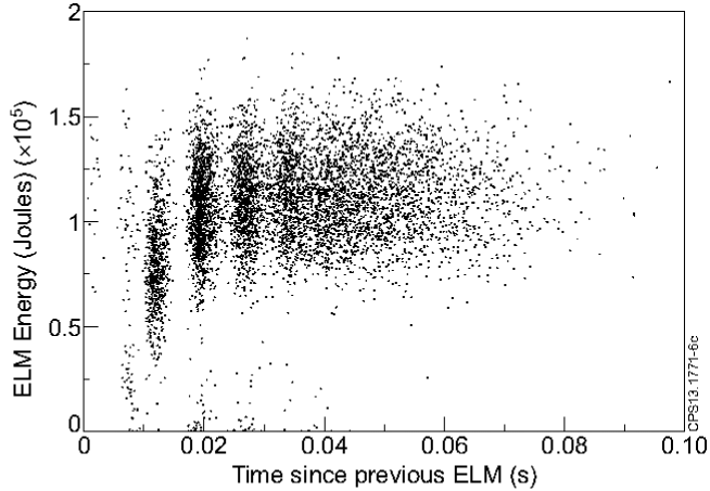
Figure 7: The drop in the plasma’s thermal energy is plotted against waiting time since the previous ELM, with $\delta E$ calculated using $t_{m}=$ 0.01 seconds. The vertical clustering is due to the unusual ELM waiting time pdf described in references EPSResonances ; Resonances , and shown in figure 1. The total stored thermal energy was of order (2.8)$\times$10⁶ Joules, so the drop in thermal energy is of order 0.04% of the plasma’s total thermal energy. Beyond 0.02 seconds the drops in energy are approximately independent of the waiting time between the ELMs.

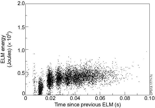
Figure 8: The drop in the plasma’s thermal energy is plotted against waiting time since the previous ELM, as in figure 7. Here however, $\delta E$ has been calculated using $t_{m}=$ 0.005 seconds, the time of the first plateau in $\delta E$ versus $t_{m}$ in figure 6, and the time beyond which the drop in edge density has ended.

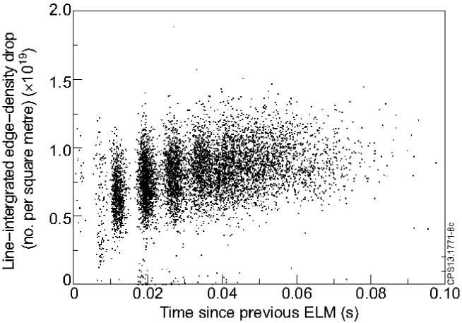
Figure 9: The drop in line integrated edge density is plotted against waiting time since previous ELM. Similarly to the plot of energy against waiting time, the vertical clustering is due to the unusual ELM waiting time pdf of the ELMs in these pulses, as described in references EPSResonances ; Resonances . The line-integrated edge density was of order (4.5).10¹⁹, suggesting that roughly 20% of the edge density is lost per ELM. Beyond about 0.005 seconds the minimum observed drop in density is independent of $t_{m}$. Beyond 0.02 seconds the drop in edge density due to an ELM is only very weakly dependent on the waiting time between ELMs.

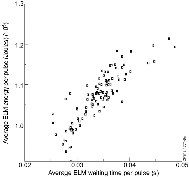
Figure 10: For each of the 120 pulses, the average of the thermal energy lost per ELM is calculated using the minimum drop in energy within 0.01 seconds of the start of each ELM, and is plotted against the average ELM waiting time for that pulse. The scatter is similar to what would be expected from the central limit theorem and the roughly 50 ELMs per pulse, indicating that the pulses are approximately statistically equivalent. The linear relationship observed between $\langle\delta E\rangle$ and $\langle\delta t\rangle$ is as expected if $\langle\delta E\rangle\propto 1/f$, but for the small range of $\langle\delta t\rangle$ here it is also what would be expected from a simple Taylor expansion of $\langle\delta E\rangle(\delta t)$, and could in principle reflect numerous possible functions of $\delta t$.

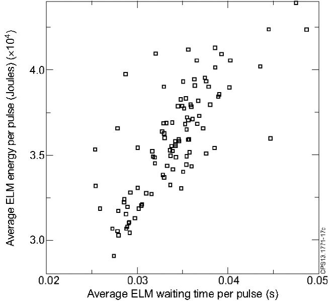
Figure 11: For each of the 120 pulses, the average of the thermal energy lost per ELM is calculated using the minimum drop in energy within 0.005 seconds of the start of each ELM, and is plotted against the average ELM waiting time for that pulse. The scatter is similar to what would be expected from the central limit theorem and the roughly 50 ELMs per pulse, indicating that the pulses are approximately statistically equivalent. The linear relationship observed between $\langle\delta E\rangle$ and $\langle\delta t\rangle$ is as expected if $\langle\delta E\rangle\propto 1/f$, but for the small range of $\langle\delta t\rangle$ here it is also what would be expected from a simple Taylor expansion of $\langle\delta E\rangle(\delta t)$, and could in principle reflect numerous possible functions of $\delta t$.

A related question is whether the energies of subsequent ELMs are related to each other, or are independent. For example, we might expect a large ELM to be followed by a smaller ELM and vice versa. Figures 12 and 13 plot the energy of the nth ELM versus the energy of the (n+1)th ELM. If a large ELM is followed by a smaller ELM and vice versa, then we would expect the plotted values to cluster around a line that is perpendicular to the diagonal. The symmetric clustering about an average ELM energy suggests that the ELM energies (surprisingly) are independent. The same result was found for $t_{m}=0.01$ seconds and $t_{m}=0.005$ seconds, and when examining $t_{n+m}$ versus $t_{n}$ for $m=1$ to $m=5$.

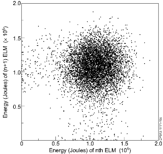
Figure 12: The energy of successive ELMs are plotted, with energies calculated using $t_{m}=0.01$. Surprisingly, the clustering of subsequent ELM energies around a single point indicates that the energies of subsequent ELMs are independent. If a large ELM were followed by a small ELM and vice versa, then we would expect a spread of ELM energies in a perpendicular direction to the diagonal.

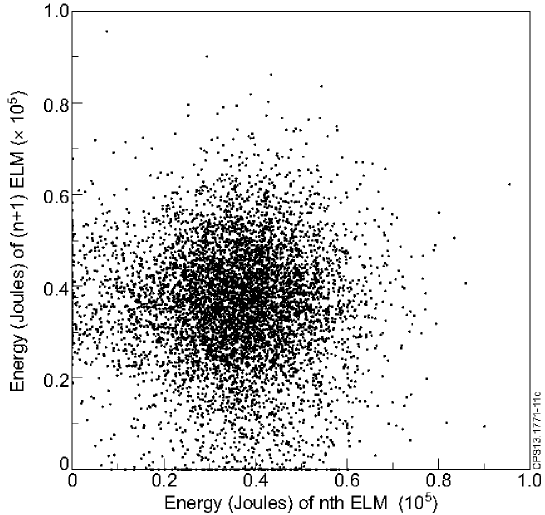
Figure 13: The energy of successive ELMs are plotted, with energies calculated using $t_{m}=0.005$. Surprisingly, the clustering of subsequent ELM energies around a single point indicates that the energies of subsequent ELMs are independent. If a large ELM were followed by a small ELM and vice versa, then we would expect a spread of ELM energies in a perpendicular direction to the diagonal.

IV Edge Temperature and Pressure Evolution

For the plasmas considered here, the edge plasma properties prevented JET’s ECE diagnostic from providing reliable edge-temperature measurements. Thompson scattering can also provide edge temperature measurements, but at present only every 50 milliseconds, that compares with the average time between ELMs of about 30-40 milliseconds for these pulses. This prevents us from determining whether the temperature and pressure drops after individual ELMs are dependent on the waiting time since the previous ELM. However we can get an approximate estimate for the average changes in edge temperature and pressure before and after ELMs by synchronising the Thompson scattering data to the ELM times and then combining all the data into a single plot. These plots of temperature, density, and pressure, are in figures 14, 15, and 16.

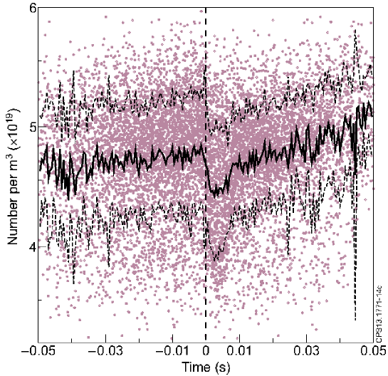
Figure 14: The Thompson scattering measurement of particle number density, averaged over the plasma edge region (between 3.74m and 3.80m along its line of sight to the magnetic axis), from all ELMs and plasma pulses, synchronised to the ELM times to allow an estimate for the density’s pre- and post-ELM evolution to be made. Brown circles are individual measurements, the thick black line is their average, and the dashed black lines are their average $\pm$ the standard deviation. The number of particles per unit volume (vertical axis) are in units of m^-3, and the horizontal time axis is in seconds. Notice that there is a minimum at around 3-5 milliseconds, as was previously observed in the line-integrated measurement (figure 3).

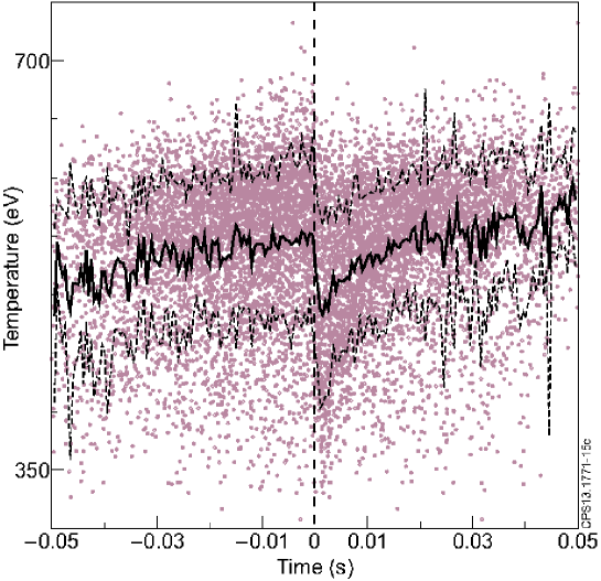
Figure 15: The Thompson scattering measurement of temperature, averaged over the plasma edge region (between 3.74m and 3.80m along its line of sight to the magnetic axis), from all ELMs and plasma pulses, synchronised to the ELM times to allow an estimate for the temperature’s pre- and post-ELM evolution to be made. Brown circles are individual measurements, the thick black line is their average, and the dashed black lines are their average $\pm$ the standard deviation. Units are eV (vertical axis), and seconds (horizontal axis). Notice that there is a minimum at around 2 milliseconds, as was similarly found in Refs. Beurskens ; Frassinetti .

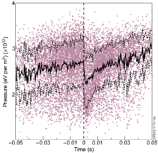
Figure 16: The Thompson scattering measurement of pressure, averaged over the plasma edge region (between 3.74m and 3.80m along its line of sight to the magnetic axis), from all ELMs and plasma pulses, synchronised to the ELM times to allow an estimate for the pressure’s pre- and post-ELM evolution to be made. Brown circles are individual measurements, the thick black line is their average, and the dashed black lines are their average $\pm$ the standard deviation. Units are eV m^-3 (vertical axis), and seconds (horizontal axis). After 20 milliseconds the pressure is approximately the same as its pre-ELM value. This partly explains why after 20 milliseconds the ELM energies are statistically the same.

The measurements shown are an average of the Thompson scattering measurements between 3.74m and 3.80m along its line of sight to the magnetic axis, which crosses a similar region to the line-integrated measurements of figure 3 (that passes vertically downwards perpendicularly through the midplane at 3.73m), and ignores measurements from the outermost edge where the Thompson scattering errors are large.

The density measurements shown in figure 14 are consistent with figure 3 (the line integrated density cuts through $\sim$1m of plasma, see Appendix A for more details), and a minimum in the post-ELM edge density is again seen at around 3-5 milliseconds after the ELM. The temperature shown in figure 15 falls to a minimum at around 2 milliseconds after an ELM, as was similarly found in Refs. Beurskens ; Frassinetti . Following an ELM, figures 14-16 give the average drop in density to be of order (0.5 $\pm$ 0.5).10¹⁹m^-3, the drop in temperature to be of order (75 $\pm$ 75)eV, and the drop in pressure to be of order (0.5 $\pm$ 0.5).10²²eVm^-3, where the error bars are the standard deviation. The volume of edge plasma that the measurements cover is of order 15m³, so for a plasma pressure $p$ and volume $V$, the thermal (“kinetic”) energy lost from the region is $(3/2)\int pdV\sim$ (3/2)(15).10²²(1.6).10^-19J$\sim$36kJ. The estimate may be a bit smaller than it should be because we have only considered changes in energy between the flux surfaces that cut 3.74m and 3.8m along the Thompson scattering’s line of sight to the magnetic axis. Note however that a 36kJ loss over 2-5 milliseconds is consistent with the time and magnitude of the first minimum in figure 4, suggesting that EFIT’s estimate for the loss in thermal (“kinetic”) plasma energy is approximately correct during the first 0-5 milliseconds of an ELM. This is reassuring. Any random errors in EFIT’s calculation for the plasma pressure will be eliminated by the subsequent averaging over large numbers of data sets; the agreement with the Thompson scattering measurement suggest that any systematic errors over this 0-5 millisecond post-ELM time-period are reasonably small. Note that the plasmas here have smaller current, smaller toroidal magnetic field, smaller heating, and consequently smaller ELMs than those in Ref. Frassinetti . The second minima in figure 4 at 10 milliseconds requires a further drop in energy by 70-100 kJ. Because the direct measurement of plasma pressure (figure 16), disagrees with EFIT’s calculated plasma pressure during the 5-10 millisecond time period after an ELM, it seems likely that EFIT’s calculations for the pressure during this time period are incorrect. As mentioned previously, the cause of the difference between the direct Thompson scattering measurements and EFIT’s calculated pressure are likely to be due to non-ideal, possibly resistive processes, that occur while the plasma is relaxing to a new post-ELM equilibrium. Returning to figures 14, 15, and 16, it is clear that after about 20 milliseconds the edge pressure has returned to very close to its pre-ELM value. There continues to be a small increase in pressure from 20 milliseconds until the next ELM, but this is small compared with the scatter in the data. This suggests a picture for these pulses where the edge pedestal is largely restored after 20 milliseconds, which helps to explain why the ELM energies are statistically similar after 20 milliseconds (figs. 7, 8, 9, 17, and 18). It also supports a picture where the ELM energy is determined by the maximum edge pressure.

V Discussion and Conclusions

We have used the line integrated edge density and the thermal energy calculated with EFIT to study the properties of the $\sim$10,000 ELMs produced from 120 (of 150) almost identical JET pulses, and have used Thompson scattering to check these results by observing the average evolution of the edge temperature and pressure in these plasmas. It is found that: i) There are clear timescales associated with the ELMs, with a loss of edge temperature over 2 milliseconds, a loss of density and pressure over 5 milliseconds, and an additional 10 millisecond timescale over which non-ideal affects appear to make EFIT’s equilibrium reconstruction unreliable. The energy losses over the shorter 2-3 milliseconds timescale appear to be associated with the loss of thermal plasma energy (“kinetic” energy), with minima in edge temperature, pressure, and density occurring within a 2-5 millisecond timescale after an ELM. The 0.005-0.01 second timescale is a previously unreported timescale during which the (ideal-MHD) plasma pressure reconstructed by EFIT disagrees with Thompson scattering measurements, and is a similar timescale to the 8 milliseconds resistive timescale of JET’s plasma pedestal (see Appendix B). This suggests that after an ELM there are non-ideal, possibly resistive processes occurring over a 5-10 millisecond timescale, as the plasma pressure and edge pedestal recover towards their pre-ELM values. It also helps to explain why for timescales of order 0-5 milliseconds, EFIT’s calculations and the Thompson scattering measurements agree. ii) Following an ELM, no ELMs are observed until approximately 0.012 seconds later, when they are statistically about 60% of the size of ELMs observed in the next cluster at approximately 0.02 seconds. Similar remarks apply regardless of whether the shorter or longer timescales of $t_{m}=$ 0.005 seconds or $t_{m}=$ 0.01 seconds are used to define the energy drop due to an ELM. iii) From 0.02 seconds onwards, the ELM energies are all statistically similar, with an approximately Gaussian distribution that is independent of the waiting times between the ELMs, and a standard deviation that is about 1/4 of the average ELM energy (see figures 17 and 18). Although the edge pressure appears to increase until an ELM, it changes very little compared with its rapid recovery in the 20 milliseconds after an ELM. This suggests that the edge pedestal is largely recovered 20 milliseconds after an ELM, consistent with the similarities in ELM energies from 20 milliseconds onwards. If the edge pressure and ELM properties are so similar from 20 milliseconds after an ELM, there are some interesting questions about: what triggers the next ELM? the proximity of the edge plasma to marginal stability? and whether the ELM trigger is better regarded as a statistical or deterministic process?

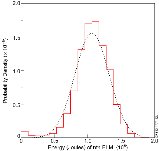
Figure 17: The probability density of ELM energies calculated with $t_{m}=0.01$ is plotted, along with a simple Gaussian fit (dotted black curve). Even without excluding the ELMs that arise with waiting times less than roughly 0.02 seconds, the distribution of ELM energies is approximately Gaussian, with an average ELM energy of (1.06)10⁵ Joules and a standard deviation of (0.26)10⁵ Joules, giving a co-efficient of variation of 0.25 for the spread of ELM energies.

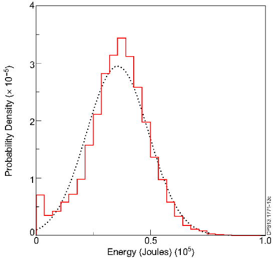
Figure 18: The probability density of ELM energies calculated with $t_{m}=0.005$ is plotted, along with a simple Gaussian fit (dotted black curve). Even without excluding the ELMs that arise with waiting times less than roughly 0.02 seconds, the distribution of ELM energies is approximately Gaussian, with an average ELM energy of (3.55)10⁴ Joules and a standard deviation of (1.35)10⁴ Joules, giving a co-efficient of variation of 0.38 for the spread of ELM energies.

The first point (i), helps to clarify the processes taking place during an ELM that need to be better understood, and includes the observation of an extra relaxation time during the ELM process. Points (ii)-(iii) have clear consequences for ELM mitigation, at least for plasmas similar to those discussed here. The maximum (natural) ELM frequency that is observed has an ELM waiting time of approximately 0.012 seconds. ELMs with waiting times of $\simeq$ 0.012 seconds have an average energy loss associated with the ELM that is roughly 60% that of the ELMs with waiting times of 0.02 seconds or longer. So presuming that ELM pacing techniques can consistently pace ELMs with waiting times of 0.012 seconds or less, then a reduction in average ELM energy by at least 40% seems likely to be possible, or 50% if we presume that the shorter timescale of $t_{m}=$ 0.005 seconds determines the peak heat fluxes onto surfaces. In principle JET can trigger ELMs with “vertical kicks” NewRef , with frequencies up to about 100Hz, so it would be possible to test this experimentally at JET using 83Hz kicks. Although we caution that even at 83Hz, the spread of the ELM energies observed in figures 6 and 7 can include energies significantly above the average observed value. To the authors’ knowledge, no vertical kick experiments have yet been done at this frequency.

If a resistive process is responsible for the 0.01 second timescale, then it might allow the energy to be lost more uniformly in the form of plasma filaments for example, possibly helping to reduce the peak heat fluxes at the divertor. The maximum heat fluxes (gradients) in figure 4 are between 0-2 milliseconds and 5-8 milliseconds, although only the heat flux calculated over 0-2 milliseconds is thought to be a reliable estimate.

The results summarised in figure 7 clearly fail to satisfy the often quoted relationship of $\delta E\propto 1/f$. This may be partly because the relationship that is measured in such papers is actually $\langle\delta E\rangle\propto 1/\langle f\rangle$, and consequently refers to average properties of possibly very different plasmas, and not to the properties of individual ELMs within similar plasmas. Unfortunately it is this latter quantity, the relationship between ELM size and ELM waiting time that is important for ELM mitigation by pacing techniques. Without a reduction in ELM energy, mitigation techniques will need to reduce either the peak heat flux or increase the wetted area onto which energy is deposited. The results presented here also only represent one particular type of pulse in one tokamak, JET. It is entirely possible that different pulse types or different machines might have very different ELM statistics. The purpose of the analysis here is to provide a robust analysis of these 2T 2MA pulses for which such large numbers of (almost) statistically equivalent ELMs are available, providing a clear indication of ELM behaviour for this particular pulse type at least. The hope was that the excellent statistics might indicate new or unexpected ELM physics. One of the unexpected results is the observed independence of ELM size and waiting time for waiting times greater than about 0.02 seconds. The generality of these results remains to be determined, and may require dedicated new experiments to ensure a robust answer.

The results here have consequences for the correct construction of models for ELMs and ELMing behaviour. For the pulses discussed here, beyond the group of ELMs with $\sim$0.012 seconds waiting time, the ELM waiting times and energies are independent. Consequently for such ELMs, models to describe their waiting times and ELM-energy probability distributions can be treated independently. Even more surprisingly perhaps, is that figures 12 and 13 suggest that the energies of subsequent ELMs are independent, so that a large ELM is as likely to be followed by another large ELM as by a small ELM. Surprising as this may be, it is likely to make the statistical modelling of ELM energies considerably easier. Clearly, the statistical relationships observed here need to be reproducable by any simulation that is correctly modelling these plasmas. Similar remarks apply to the relaxation of the plasma’s energy, and the sequence of processes and timescales by which the plasma loses energy due to an ELM.

To conclude, we have presented the analysis of an unprecedentedly large number of statistically equivalent 2T 2MA JET ITER-like wall H-mode plasmas. This has led to the observation of an extra 0.01 second timescale associated with the ELM process, that is consistent with a resistive mechanism that allows the plasma to relax to a new post-ELM equilibrium. For the plasmas discussed here, surprising results are reported about the independence of ELM energy and frequency, and the independence of energies of consecutive ELMs. Whether the results found here are more generally true is unknown, it may be some time before equivalently large datasets for different pulse types or from different machines become available.

Appendix A Plasma motion and measurements

Following an ELM there will be a radial motion of the plasma. This will modify the measurements in two ways: i) the length of plasma that the line-integrated measurements pass through will reduce slightly, ii) the measurements will be of a slightly different region of plasma due to its small radial displacement. Here we will estimate the changes to measurements that would be expected to result from a small radial displacement of the plasma, and confirm that they are small compared to the measured changes that occur after an ELM, and can therefore be neglected.

During an ELM the radial outer gap between the outboard plasma and the outer wall changes by 7-8mm, which is 0.007-0.008m. The line integrated measurement passes through approximately 1.45m of plasma, approximately 1.1m of which is through the higher density region above the top of the plasma pedestal (these lengths can be used to estimate the plasma density from the line-integrated density measurement). Allowing for the geometry of the flux surfaces, a 7-8mm radial shift will only modify the length of plasma it passes through by a few cms at the most, or by 1-2%. Therefore because the measured changes in line-integrated density are of order 10-20%, we can neglect this effect.

The edge pedestal is thought to be 2-3cms at most Frassinetti2 , and the line-integrated measurement cuts through the mid-plane at about 3.73m, so most of the line of sight is through plasma above the top of the pedestal (at the mid-plane the plasma edge is at approximately 3.80m). Above the top of the pedestal the plasma density gradient is between 2.10¹⁹m^-4 and 5.10¹⁹m^-4, so a 0.008-0.009m ROG shift will change the density that is measured by the line-integrated measurement by less than (0.05).10¹⁹m^-3, which is less than 1%. Therefore because the measured changes in line-integrated density are by 10-20%, we can neglect this affect also.

In summary, compared with the measured changes in density, the changes due to the radial plasma shift that occurs with an ELM can be neglected. Similar remarks apply to the temperature and pressure measurements.

Appendix B The current relaxation timescale

As given in Ref. Friedberg for example, the plasma’s resistivity is,

$$\eta=(6.5)10^{-8}\left(\frac{1}{T_{k}^{3/2}}\right)\mbox{ $\Omega$ m}$$ (1)

where $T_{k}$ is the plasma’s temperature measured in electron Volts. A multiplicative constant modifies Eq. 1 when Neoclassical effects are included and if $Z_{eff}\neq 1$, but Eq. 1 is a reasonable order of magnitude estimate. The resistive MHD equations Friedberg give,

$$\frac{\partial\vec{B}}{\partial t}=\left(\frac{\eta}{\mu_{0}}\right)\nabla^{2}\vec{B}$$ (2)

from which a dimensional analysis gives the resistive timescale $\tau$ as,

$$\tau\sim\left(\frac{\mu_{0}}{\eta}\right)L^{2}$$ (3)

where $L$ is a typical length scale and $\mu_{0}=(4\pi)10^{-7}$ Farad m^-1. Combining equations 1 and 3 gives,

$$\tau\sim(6.2)\pi T_{k}^{3/2}L^{2}$$ (4)

Substituting the pedestal width Frassinetti2 of $L\sim 0.03$m and temperature at the pedestal’s top of $T_{k}\sim 0.6$keV, gives $\tau\sim 8$ milliseconds, very similar to the $10$ millisecond timescale observed in figures 4 and 6.

References

- (1) J. Wesson Tokamaks (Oxford University Press, Oxford, 1997).
- (2) P.B. Snyder, R.J. Groebner, A.W. Leonard, T.H. Osbourne, H.R. Wilson, Phys. Plasmas 16, 056118, (2009).
- (3) A.J. Webster, Nucl. Fusion 52, 114023, (2012).
- (4) M. Keilhacker, Plasma Phys. Control. Fusion, 26, 49 (1984).
- (5) H. Zohm, Plasma Physics and Controlled Fusion 38, 105, (1996).
- (6) Kamiya et al., Plasma Physics and Controlled Fusion 49, S43, (2007).
- (7) R. Aymar et al. for THE ITER TEAM, Plasma Physics and Controlled Fusion 44, 519, (2002).
- (8) B. Lipschultz, X. Bonnin, G. Counsell, et al. Nucl. Fusion 47, 1189-1205, (2007).
- (9) A. Loarte, B. Lipschultz, A.S. Kukushkin, et al. Nucl. Fusion 47, S203-263, (2007).
- (10) P.T. Lang, A. Loarte, G. Saibene, et al. Nucl. Fusion 53, 043004, (2013).
- (11) Y. Liang, Fusion Science and Technology 59, 586, (2011).
- (12) A. Herrmann, Plasma Phys. Control. Fusion 40, 883-903, (2002).
- (13) R. Neu, G. Arnoux, M. Beurskens, et al. Phys. Plasmas 20, 056111, (2013).
- (14) G.P. Maddison, C. Giroud, B. Alper, et al. Nucl. Fusion 54, 073016, (2013).
- (15) S. Brezinsek, T. Loarer, V. Phillips, et al. Nuclear Fusion, 53, 083023, 2013.
- (16) A.J. Webster, R.O. Dendy, F.A. Calderon, S.C. Chapman, E. Delabie, D. Dodt, R. Felton, T.N. Todd, V. Riccardo, B. Alper, S. Brezinsek, P. Coad, J. Likonen, M. Rubel, and JET EFDA Contributors “The Statistics of Edge Localised Modes”, P4.112, 40th EPS Conference on Plasma Physics, Helsinki, Finland, 2013.
- (17) A.J. Webster, R.O. Dendy, F.A. Calderon, S.C. Chapman, E. Delabie, D. Dodt, R. Felton, T.N. Todd, V. Riccardo, B. Alper, S. Brezinsek, P. Coad, J. Likonen, M. Rubel, and JET EFDA Contributors, “Time-Resonant Tokamak Plasma Edge Instabilities?”, (arXiv:1310.0287), Plasma Phys. Control. Fusion, in press, (2013).
- (18) L.L. Lao, H. St. John, R.D. Stambaugh, A.G. Kellman and W. Pfeiffer, Nucl. Fusion 25, 1611, (1985).
- (19) L.C. Appel, G.T.A. Huysmans, L.L. Lao, et al. 33rd EPS Conference on Plasma Phys. Rome, 19 - 23 June 2006 ECA Vol.30I, P-2.184 (2006).
- (20) A.J. Webster and R.O. Dendy, Phys. Rev. Lett. 110, 155004, (2013).
- (21) M.N.A. Beurskens, L. Frassinetti, C. Maggi, et al. Fusion Energy 2012 (Proc. 24th Int. Conf. San Diego, 2012) (Vienna: IAEA) CD-ROM file [FEC-2012] and http://www-naweb.iaea.org/napc/physics/FEC/FEC2012/html/proceedings.pdf
- (22) L. Frassinetti, D. Dodt, M.N.A. Beurskens, et al. 40th EPS Conference on Plasma Physics, P5.183, (2013).
- (23) H. Thomsen, T. Eich, S. Devaux, et al. Nucl. Fusion 51, 123001, (2011).
- (24) L. Frassinetti, M.N.A. Beurskens, R. Scannell et al. Rev. Sci. Instrum. 83, 013506, (2012).
- (25) P.T. Lang, M. Bernert, A. Burckhart, et al. 40th EPS Conference on Plasma Physics, O2.102, (2013).
- (26) P.T. Lang, D. Frigione, A. Geraud, et al. Nucl. Fusion 53, 073010, (2013).
- (27) J. Freidberg “Plasma Physics and Fusion Energy”, Cambridge University Press, Cambridge, UK, (2007).
- (28) E. de la Luna, G. Saibene, H. Thomsen, et al. ”Effect of ELM mitigation on confinement and divertor heat loads on JET”, EXC/8-4, Fusion Energy 2012 (Proc. 24th Int. Conf. San Diego, 2012) (Vienna: IAEA) CD-ROM file [FEC-2012] and http://www-naweb.iaea.org/napc/physics/FEC/FEC2012/html/proceedings.pdf