Decoherence in a fermion environment: Non-Markovianity and Orthogonality Catastrophe

Abstract

We analyze the non-Markovian character of the dynamics of an open two-level atom interacting with a gas of ultra-cold fermions. In particular, we discuss the connection between the phenomena of orthogonality catastrophe and Fermi edge singularity occurring in such a kind of environment and the memory-keeping effects which are displayed in the time evolution of the open system.

1. Introduction and Motivations

The precise definition and quantitative description of memory effects (or non-Markovianity) have become a central issue in the theory of open quantum systems [1, 2, 3, 4, 5, 6, 7, 8, 9, 10, 11], and have been the subject of recent experimental efforts [12]. It has been argued that non-Markovianity has the potential of being exploited to pursue new quantum technologies [9], and that it can be thought as a resource in quantum metrology [13], for the generation of entangled states [14] and for quantum key distribution [15].

Various characterizations of the non-Markovian behavior have been given, which capture different aspects of the decohering dynamics of an open system. They include the lack of divisibility of the map describing the time evolution of the system of interest [1, 4], or the back-flow of the information that the system itself had previously lost, described either in terms of the distinguishability of the evolved states [2] or of the quantum Fisher information [5]. Further proposals have been put forward, based on the decay rates entering the master equation [6], on the use of the quantum mutual information [8] or of channel capacities [9], on spectral considerations [10], and on the temporary expansion of the volume of the states accessible through the reduced dynamics [16]. Moreover, many other properties, related to the locality [17], to the complexity [18] or to the size of the environment [19], have been investigated in different physical settings, ranging from spin systems [20, 21] to Bose-Einstein condensates of ultra-cold atoms [22].

Despite the conceptual differences, several quantifiers of the amount of non-Markovianity give similar qualitative (and sometimes also quantitative) descriptions when applied to the dynamics of simple quantum systems such as a qubit[23, 21]. In particular, this holds true for the specific case of a purely dephasing dynamics where the system loses coherence due to its interaction with the environment, without any energy exchange. In this case, indeed, the open system evolution is completely characterized by a so called decoherence factor, which is the only ingredient necessary to evaluate the amount of non-Markovianity.

Specifically, let us consider a two-level system (a qubit, with energy eigenstates $\left|\alpha\right\rangle$, $\alpha=0,1$) interacting with its environment in such a way as to preserve its energy. This implies that the interaction Hamiltonian commutes with that of the qubit and, as a result, the qubit state can be written as

$$\rho(t)=\begin{pmatrix}\rho_{00}(0)&\nu(t)\rho_{01}(0)\\ \nu^{*}(t)\,\rho_{10}(0)&\rho_{11}(0)\end{pmatrix},\quad\nu(t)=Tr_{env}\{e^{iH_{1}t}\,e^{-iH_{0}t}\,\rho_{env}\}\,,$$ (1)

where $\rho_{env}$ is the initial state of the environment, while $H_{\alpha}=H_{env}+\left\langle\alpha\right|H_{int}\left|\alpha\right\rangle$ are effective Hamiltonians for the environment, conditioned on the state of the qubit ($\alpha=0,1$).

If the initial state of the environment is pure, $\rho_{env}=\left|\phi\right\rangle\left\langle\phi\right|$, then the decoherence factor (whose square is known as the Loschmidt echo, $L(t)=\left|\nu(t)\right|^{2}$ [24]) is given by the overlap $\nu(t)=\left.\left\langle\phi_{1}(t)\right|\phi_{0}(t)\right\rangle$, where $\left|\phi_{\alpha}\right\rangle=e^{-iH_{\alpha}t}\left|\phi\right\rangle$.

The quantity $\nu(t)$ can be used to characterize the environment itself, and, in particular, it gives a very peculiar behavior for fermionic environment. Indeed, as first pointed out by P. W. Anderson over 40 years ago, such an overlap of the two many-body wavefunctions, describing deformed and un-deformed Fermi seas, respectively, scales with the size of the environment and vanishes in the thermodynamic limit, giving rise to an ‘orthogonality catastrophe’ [25]. The dynamic counterpart of Anderson’s theory was investigated a few years later with the prediction of a universal absorption-edge singularity in the X-ray spectrum of simple metals, which has become known as the ‘Fermi-edge singularity’ [26]. Mahan, Nozieres and De Dominicis (MND) obtained an expression for the function $\nu(t)$ describing the response of a Fermi gas to the sudden switching of a local perturbation, i.e. a core-hole induced by the X-ray, which gives rise to a deformation (or shake up) of the many body state of the gas.

It is our aim in this paper to study the analogous of such a phenomenon for a trapped gas of ultra-cold Fermi atoms in which the very fast excitation of an impurity atom (e.g. by a focused laser pulse) produces a sudden local perturbation [27, 28, 29]. The time response of the gas is directly related to the decoherence of the impurity, which experiences a purely dephasing dynamics. As mentioned above, for such a case the non-Markovianity of the map is strictly connected to the decoherence factor. As a result, with our theoretical construction we are able to explore the link between the non-Markovianity and the orthogonality catastrophe occurring within the environment.

We will adopt the geometric measure recently put forward by some of us in Ref. [16], which allows for an intuitive visualization of the information exchange between system and environment. This is briefly recalled in Sect. 2.. Then, after the model for the fermionic bath is explicitly described in Sec. 3., in Sec. 4. we use the geometric measure to discuss the decoherence of the impurity. Some final remarks are given in Sec. 5..

2. Geometric description of non-Markovianity

In this section we briefly review the definition and meaning of the measure of non-Markovianity introduced in Ref. [16], adapting it to the case of a qubit undergoing a purely dephasing dynamics. The basic idea is that the time evolution of the density matrix of a qubit can always be recast into the form of an affine transformation for the Bloch vector $\mbox{\boldmath$b$}=\mbox{Tr}\{\mbox{\boldmath$\sigma$}\}$ (where $\sigma$ is the vector of Pauli matrices), which can be contracted, rotated and translated by a given amount. In particular, for the time evolution given in Eq. (1), the translation term is absent and we have

$$\mbox{\boldmath$b$}(t)=A_{t}\,\mbox{\boldmath$b$}(0)\,,$$ (2)

with

$$A_{t}=\left(\begin{matrix}\mathfrak{Re}\nu(t)&\mathfrak{Im}\nu(t)&0\\ -\mathfrak{Im}\nu(t)&\mathfrak{Re}\nu(t)&0\\ 0&0&1\end{matrix}\right)\,.$$ (3)

The generic initial state for the qubit corresponds to a Bloch vector lying within the unit (Bloch) sphere. The set of accessible states changes as a function of time, being contracted (with respect to the initial sphere) in the equatorial plane for the case of a purely dephasing evolution. In Fig. 1 we provide a representation of this set as a function of time for two specific situations which will be described in more detail in the next section.

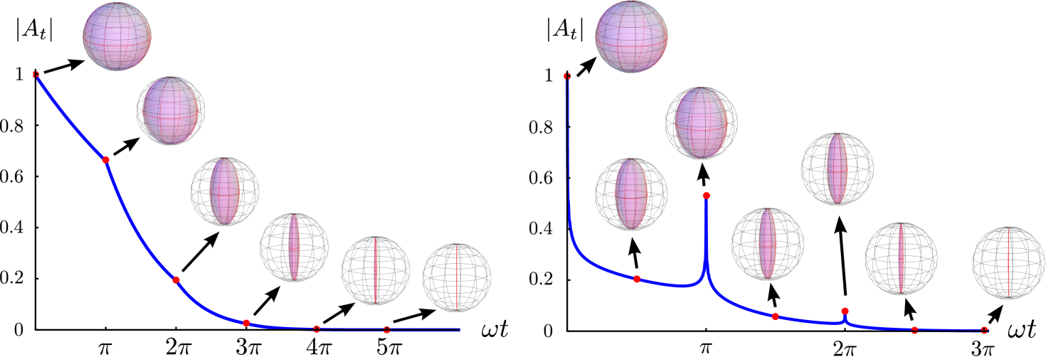
Fig. 1: Behavior of the determinant $|A_{t}|$, of the dynamical map governing the time evolution of the two-level impurity atom, for the case of an environment with $N_{F}=200$ fermions and for $\beta=0.05$ , $\alpha=0.001$ (left plot) and $\beta=3$ , $\alpha=0.1$ (right plot). (Energies are in units of $\hbar\omega$).

In the general case, the absolute value of the determinant of the matrix describing the dynamical map, $||A_{t}||$, gives the ratio between the volume of the set of states (or, more precisely, the set of $b$ vectors) accessible by the system at time $t$ and the volume of the initial set of all possible Bloch vectors, which is the entire Bloch sphere.

A dynamical map described by a Lindblad-like master equation gives rise to a non-increasing volume [1, 16]. This is true even if the master equation has time decay coefficients, provided that the latter are strictly positive quantities [30]. Hence, it is natural to call a process Markovian if the determinant does not increase in time, and non-Markovian if an initial volume contraction is followed by a temporary inflation, giving rise to a determinant that has a positive time derivative in some specific interval.

The two examples reported in Fig. 1 explicitly depict a Markovian and a non-Markovian evolution in terms of the determinant.

Using the same method adopted in Ref. [2] to single out the intervals in which the determinant increases in time, we define [16]

$$\mathcal{N}_{V}=\int_{\frac{d\left||A_{t}|\right|}{dt}>0}\frac{d\left||A_{t}|\right|}{dt}\,dt$$ (4)

as a non-Markovianity measure.

For the map corresponding to a dephasing evolution, the determinant is related to the decoherence factor. Explicitly, $\left||A_{t}|\right|=|\nu(t)|^{2}$. In Section 4., we will discuss the behavior of ${\cal N}_{V}$ for a qubit in a fermionic environment as a function of the coupling strength and of the temperature of the environment.

3. Impurity in a Fermionic environment

The explicit model for the environment that we discuss in this paper is given by a gas of ultra-cold non-interacting fermionic atoms, trapped in an harmonic potential of frequency $\omega$. This is described by the Hamiltonian

$$\hat{H}_{env}=\sum_{n}\varepsilon_{n}{c}_{n}^{\dagger}{c}_{n}\,,$$

with $c_{n}$ being the annihilation operator for the $n$-th single particle level of energy $\varepsilon_{n}=\hbar\omega(n+1/2)$. $\hat{H}_{env}$, together with the number operator $\hat{N}=\sum_{n}{c}_{n}^{\dagger}{c}_{n}$, also sets the initial equilibrium state of the gas, $\rho_{env}=\exp\{-\beta(\hat{H}_{env}-\mu\hat{N})\}/Z$, where the chemical potential $\mu$ is fixed by the requirement that the gas contains (on average) $N_{F}$ fermions, while $\beta$ is the inverse temperature.

We consider a two-level impurity, trapped in an auxiliary potential and brought in contact with the Fermi gas. We assume that when the impurity is in the state $|0\rangle$, it has a negligible scattering interaction with the gas. On the other hand, if the impurity is in the state $\left|1\right\rangle$, the gas feels a localized perturbation $\hat{V}$, describing a neutral $s$-wave like interaction that we treat in the pseudo-potential approximation: $V(x)=\pi V_{0}x_{0}\delta(x)$ (the trap length $x_{0}$ as well as the factor $\pi$ are put in the definition for future convenience only). The interaction Hamiltonian, then, has the form

$$H_{int}=\hat{V}\otimes\left|e\right\rangle\left\langle e\right|\,.$$ (5)

As mentioned in the introduction, the key quantity for our discussion is the decoherence factor

$$\nu(t)=\left\langle e^{\frac{i}{\hbar}\hat{H}_{env}t}{\,}e^{-\frac{i}{\hbar}(\hat{H}_{env}+\hat{V})t}\right\rangle\text{,}$$ (6)

where the braket symbol is a short-hand notation for the thermal equilibrium average over the unperturbed environment.

An analytic estimate can be given for this quantity both at zero and at finite temperatures [28]. Here, we will proceed to a numerical evaluation of the decoherence factor (and, in particular, of its modulus) using the linked cluster theorem and up to two-vertices connected Feynman diagrams, which amount to a partial re-summation of a perturbative expansion in the ratio of the interaction strength $V_{0}$ with the Fermi energy $\varepsilon_{F}=\hbar\omega(N_{F}+\frac{1}{2})$. The details of this kind of evaluation are given in Ref. [28], where it is shown that a good indicator of the effect of the perturbation induced on the Fermi gas is the a-dimensional parameter

$$\alpha=\frac{V_{0}^{2}}{\hbar\omega\,\varepsilon_{F}}\,.$$ (7)

This coincides with the critical parameter of the MND theory, which is obtained as the limiting case of a free Fermi gas, $\omega\rightarrow 0$.

In the following, we will consider spin $1/2$ fermions, fix their number to $N_{F}=200$, and discuss the behavior of the measure of non-Markovianity ${\cal N}_{V}$ as a function of $\alpha$ and of the inverse temperature $\beta=\frac{1}{KT}$.

4. Non-Markovianity and its relation to the shake-up of the Fermi gas

The parameter $\alpha$ introduced in the previous section is a measure of the strength of the perturbation due to the switching impurity. One could naively expect that by increasing $\alpha$ the amount of non-Markovianity in the dynamics of the qubit should increase. However, this is not the case as Fig. 2 clearly shows. In particular, ${\cal N}_{V}$ increases for a very small $\alpha$, reaching a maximum value for $\alpha\leq 0.2$, which depends on the chosen value of $\beta$. After such a maximum, ${\cal N}_{V}$ decreases with increasing the interaction strength.

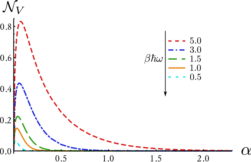
Fig. 2: Non-Markovianity measure ${\cal N}_{V}$ as function of the effective coupling strength $\alpha$, for various values of the inverse thermal energy $\beta$ expressed in units of $1/\hbar\omega$.

This is due to the peculiar way a fermionic system responds to the perturbation, especially at small temperatures. For very small $\alpha$, an almost linear increase with the intensity of the perturbation is expected from simple second order perturbation theory. Indeed, to first order in $V_{0}$ one would obtain only a shift of the energy levels, resulting in a purely oscillating $\nu(t)$; the second order correction in $V_{0}$ (which are linear in $\alpha$), instead, introduces a distortion of the single-particle energy eigenstates.

A small $\alpha$ implies that the Fermi surface is not substantially modified and that only those fermions whose energy is close to the Fermi energy are excited. This, in turns, means that only a few fermionic modes (and, thus, few almost undistorted frequencies) enter the dynamics, and give rise to a quasi-periodicity of the function $\nu(t)$ with frequency $\omega$. As a result, every half a period the derivative of the determinant changes sign and a contribution is given to the integral in Eq. (4). The accumulation of such positive contributions gives rise to an ${\cal N}_{V}$ that grows with $\alpha$. Notice, however, that a true periodicity is quickly lost with increasing $\alpha$, especially if the temperature is not kept low. From Fig. 1, one can see that only a vague periodicity survives already at $\alpha=0.1$ if $KT=\hbar\omega/3$.

This increase of ${\cal N}_{V}$ with increasing $\alpha$ is counteracted by an effective suppression of the oscillations in $\nu(t)$ which occurs when the single-particle energies become more and more distorted (so that they are not anymore multiple of $\omega$) and when more and more transitions are induced by the increasing-in-strength of the perturbation. For large values of $\alpha$, indeed, the entire Fermi sea responds to the perturbation and the non-markovianity decreases.

Such a behavior can be also interpreted in a complementary way. For small $\alpha$’s the effective environment felt by the impurity has a very prominent spectral structure, given by the Fermi edge. On the other hand, with increasing $\alpha$, the effective environmental frequency spectrum becomes more and more flat, giving rise to an effective Markovian dynamics for the qubit.

This line of reasoning is confirmed by the fact that the amount of non-Markovianity decreases with increasing the temperature due to the fact that the Fermi edge is more and more blurred for a smaller and smaller $\beta$.

Fig. 3 gives the behavior of the amount of non-Markovianity as function of the trap frequency, to explicitly confirm that ${\cal N}_{V}$ increases with $\omega$ as a result of the fact that the periods in which the determinant grows become closer to each other in time.

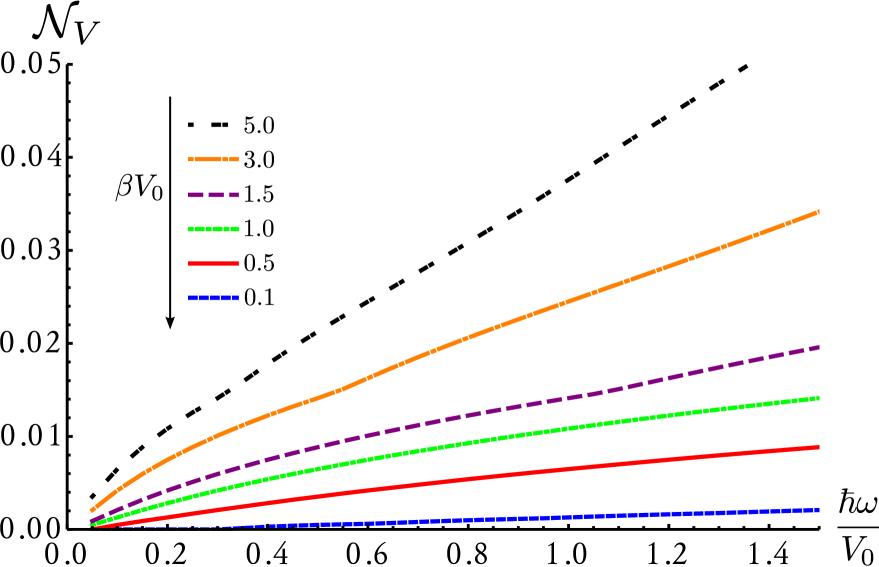
Fig. 3: Non-Markovianity measure as function of the trap frequency $\omega$ for different temperatures.

In particular, for the free gas originally treated by MND, which is obtained when $\omega\rightarrow 0$, the dynamics of the impurity is fully markovian due to the absence of any oscillations in the decoherence factor.

4.1. Build-up in time of the non-Markovianity

The non-Markovianity measure ${\cal N}_{V}$ gives an integral characterization of the whole dynamics. More details on the time development of the memory effects during the system-environment information-exchange process can be obtained if we consider separately the time intervals in which the determinant increases and decreases, up to a given time $t$. To this end, it is useful to define

$$\mathcal{N}_{\pm}(t)=\pm\int_{\pm\frac{d\left||A_{\tau}|\right|}{d\tau}>0}\frac{d\left||A_{\tau}|\right|}{d\tau}\,\theta(t-\tau)\,d\tau\,,$$ (8)

which give, respectively, (the sum of ) the amount of expansion/contraction of the volume of the set of accessible states within the time $t$. In particular, it is meaningful to consider the ratio

$${\cal R}(t)=\frac{N_{+}(t)}{N_{-}(t)}\,,$$ (9)

which expresses the fraction of the volume which is recovered in the expansions with respect to the one lost due to the previous contractions. The function ${\cal R}(t)$ is strictly zero until the volume starts increasing and then it grows/diminishes with the volume. Every time interval in which ${\cal R}$ grows corresponds to a positive contribution to the build-up of the integral measure ${\cal N}_{V}$.

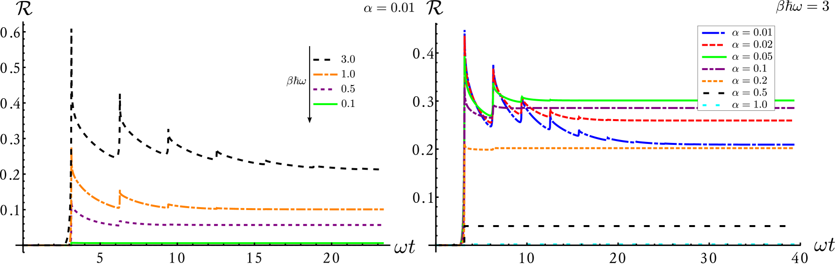
Fig. 4: Ratio expansion over contraction factors of the volume of states accessible through the dynamical map after time $t$. The left panel reports ${\cal R}(t)$ at fixed $\alpha=0.01$ for various temperatures, while the right panel shows the same quantity for different values of $\alpha$ and a fixed $KT=\hbar\omega/3$.

Fig. 4 confirms the interpretation that the non-Markovianity is due to quasi-periodic oscillations of the volume of the set of accessible states, occurring with a period $2\pi/\omega$, which is more and more suppressed with increasing temperature

5. Concluding remarks

In this paper we studied the dynamics of a two-level impurity encapsulated in a trapped fermion environment. Due to the presence of the Fermi edge, at low temperatures such an environment enjoys the presence of a spectral structure which induces a non-Markovian behavior in the time evolution of the impurity. This is due to the oscillating response of the trapped Fermi gas in which transition are induced by the perturbing local impurity. Such a behavior is found to occur provided the interaction strength is not too large (with respect to the relevant energy scale of the gas, given by $\sqrt{\varepsilon_{F}\hbar\omega}$). On the other hand, a stronger interaction tends to smoothen the environmental spectral density giving rise to a Markovian dynamics for the impurity. Markovianity is generically obtained also if the temperature is larger than the scale set up by the trapping frequency and, more generally, whenever the discrete structure of the single-particle energy levels of the gas can be confused with a continuum, e. g. in the absence of the trap.

The effects that we reported can be studied with a system of trapped cold fermionic atoms. Indeed, in this realm, many experiments have recently dealt with the effect of impurities within the gas [31], which can be easily tested both as function of the interaction strength (changeable via the phenomenon of Feshbach resonance) and of the trapping frequency.

References

- [1] M. M. Wolf, J. Eisert, T. S. Cubitt, and J. I. Cirac, Phys. Rev. Lett. 101, 150402 (2008).
- [2] H.-P. Breuer, E.-M. Laine, J. Piilo, Phys. Rev. Lett. 103, 210401 (2009).
- [3] D. Chruscinski and A. Kossakowski, Phys. Rev. Lett. 104, 070406 (2010).
- [4] À. Rivas, S.F. Huelga, and M.B. Plenio, Phys. Rev. Lett. 105, 050403 (2010).
- [5] X.-M. Lu, X. Wang, and C. P. Sun, Phys. Rev. A 82, 042103 (2010)
- [6] E. Andersson, J. D. Cresser, and M. J. W. Hall, arXiv:1009.0845 (2010).
- [7] R. Vasile, S. Maniscalco, M. G. A. Paris, H.-P. Breuer, and J. Piilo, Phys. Rev. A 84, 052118 (2011).
- [8] S. Luo, S. Fu, and H. Song, Phys. Rev. A 86, 044101 (2012).
- [9] B. Bylicka, D. Chruściński, and S. Maniscalco, arXiv:1301.2585.
- [10] W.-M. Zhang et al., Phys. Rev. Lett. 109, 170402 (2012).
- [11] H.-P. Breuer, J. Phys. B: At. Mol. Opt. Phys. 45, 154001 (2012).
- [12] B.-H. Liu, L. Li, Y.-F. Huang, C.-F. Li, G.-C. Guo, E.- M. Laine, H.-P. Breuer, and J. Piilo, Nat. Phys. 7, 931 (2011); A. Chiuri, C. Greganti, L. Mazzola, M. Paternostro, and P. Mataloni, Sci. Rep. 2, 968 (2012); B.-H. Liu, D.-H. Cao, Y.-F. Huang, C.-F. Li, G.-C. Guo, E.-M. Laine, H.-P. Breuer, J. Piilo, Scientific Reports 3, 1781 (2013).
- [13] A. W. Chin, S. F. Huelga, and M. B. Plenio, Phys. Rev. Lett. 109, 233601 (2012).
- [14] S. F. Huelga, Á. Rivas, M. B. Plenio, Phys. Rev. Lett. 1085, 160402 (2012).
- [15] R. Vasile, S. Olivares, M. G. A. Paris, S. Maniscalco, Phys. Rev. A 83, 042321 (2011).
- [16] S. Lorenzo, F. Plastina, and M. Paternostro, Phys. Rev. A (R) 88, 020102 (2013).
- [17] E.-M. Laine, H.-P. Breuer, J. Piilo, C.-F. Li, and G.-C. Guo, Phys. Rev. Lett. 108, 210402 (2012).
- [18] M. Žnidarič, C. Pineda, and I. García-Mata, Phys. Rev. Lett. 107, 080404 (2012); I. García-Mata, C. Pineda, D. Wisniacki Phys. Rev. A 86, 022114 (2012).
- [19] S. Lorenzo, F. Plastina, and M. Paternostro, Phys. Rev. A 87, 022317 (2013).
- [20] T. J. G. Apollaro et al., Phys. Rev. A 83, 032103 (2011).
- [21] P. Haikka, J. Goold, S. McEndoo, F. Plastina, and S. Maniscalco, Phys. Rev. A 85, 060101(R) (2012);
- [22] P. Haikka, S. McEndoo, G. De Chiara, G. M. Palma, and S. Maniscalco, Phys. Rev. A 84, 031602(R) (2011); P. Haikka, S. McEndoo, and S. Maniscalco, Phys. Rev. A 87, 012127 (2013).
- [23] H.-S. Zeng et al., Phys. Rev. A 84, 032118 (2011).
- [24] A. Peres, Phys. Rev. A 30, 1610 (1984); T. Gorin et al., Phys. Rep. 435, 33 (2006); F. M. Cucchietti, et al., Phys. Rev. Lett. 91, 210403 (2003); P. Zanardi and N. Paunkovíc, Phys. Rev. E. 74, 031123 (2006).
- [25] P. W. Anderson, Phys. Rev. Lett. 18, 1049 (1967).
- [26] G.D. Mahan, Phys. Rev. 163, 612 (1967); P. Nozieres and C.T. De Dominicis, Phys.Rev. 178, 1097 (1969).
- [27] J. Goold, T. Fogarty, N. Lo Gullo, M. Paternostro, and T. Busch, Phys. Rev. A 84, 063632 (2011).
- [28] A. Sindona et al., Phys. Rev. Lett. 111, 165303 (2013).
- [29] M. Knap et al., Phys. Rev. X 2, 041020 (2012).
- [30] J. Piilo, S. Maniscalco, K. Härkönen, and K.-A. Suominen, Phys. Rev. Lett. 100, 180402 (2008).
- [31] A. Schirotzek et al., Phys. Rev. Lett. 102, 230402 (2009); C. Kohstall et al., Nature 485, 615 (2012); M. Koschorreck et al., Nature 485, 619 (2012).