Statistical properties of 1D parametrically kicked Hamilton systems

Abstract

We study the 1D Hamiltonian systems and their statistical behaviour, assuming the initial microcanonical distribution and describing its change under a parametric kick, which by definition means a discontinuous jump of a control parameter of the system. Following a previous work by Papamikos and Robnik J. Phys. A: Math. Theor. 44 (2011) 315102 we specifically analyze the change of the adiabatic invariant (the action) of the system under a parametric kick: A conjecture has been put forward that the change of the action at the mean energy always increases, which means, for the given statistical ensemble, that the Gibbs entropy in the mean increases. By means of a detailed analysis of a great number of case studies we show that the conjecture largely is satisfied, except if either the potential is not smooth enough, or if the energy is too close to a stationary point of the potential (separatrix in the phase space). Very fast changes in a time dependent system quite generally can be well described by such a picture and by the approximation of a parametric kick, if the change of the parameter is sufficiently fast and takes place on the time scale of less than one oscillation period. We discuss our work in the context of the statistical mechanics in the sense of Gibbs.

I Introduction

In a recent work Papamikos and Robnik Papamikos and Robnik (2011) have studied time dependent nonlinear Hamiltonian oscillators from the point of view of their statistical properties, in order to generalize a series of studies on the time dependent linear oscillator by Robnik and Romanovski Robnik and Romanovski (2006a, b); Robnik et al. (2006); Kuzmin and Robnik (2007); Robnik and Romanovski (2008), where the rigorous WKB method has been employed Robnik and Romanovski (2000). We are interested in the time evolution of a microcanonical ensemble of initial conditions. If the evolution is ideal adiabatic (i.e. infinitely slow), then the adiabatic invariant, which is also the action of the system, or the area inside the contour of constant energy in the phase space (divided by $2\pi$), is conserved, and this is precisely the adiabatic theorem on one-dimensional Hamiltonian systems Arnold (1989), provided we do not cross a separatrix during the adiabatic process. What happens if the changing of the system parameter is not adiabatic? For the linear oscillator with an arbitrary time dependence it has been shown rigorously in the above mentioned papers (see in particular the review Robnik and Romanovski (2008)) that the value of the adiabatic invariant at the average value of the energy during the evolution is always increasing. Since the adiabatic invariant is proportional to the number of states, this implies an irreversibility in the mean, because the entropy is the logarithm of the number of states, in the sense of statistical mechanics, as explained in section 2. This finding was a motivation to analyze the nonlinear oscillators from this point of view. In Papamikos and Robnik (2011) it was shown using the numerical techniques (highly accurate symplectic integrators of 8th order, McLachlan (1995); McLachlan and Quispel (2002); Hairer et al. (2006); Leimkuhler and Reich (2004); Senz-Serna and Calvo (1994); Shimada and Yoshida (1996); Yoshida (1990, 1993); Papamikos (2011)) that for slow but not adiabatic changes in a quartic oscillator the adiabatic invariant at the mean energy can decrease, just due to the nonlinearity and nonisochronicity. However, for sufficiently fast changes the property is restored, especially in the extreme case of a parametric kick, when the system’s parameter jumps discontinuously. This led us to demonstrate analytically by a rigorous calculation for the case of homogeneous power law potentials (of which the quartic oscillator and the harmonic oscillators are two special cases), that the adiabatic invariant at the average final energy indeed increases under a parametric kick.

Therefore, we Papamikos and Robnik (2011) have put forward a Conjecture (henceforth called PR Conjecture) that the adiabatic invariant for an initial microcanonical ensemble at the mean energy always increases under a parametric kick. The purpose of the present work is to investigate the validity and the conditions under which it is true. We show by a series of case studies, that the PR Conjecture is largely true, except if either the potential is not smooth enough, or if the energy is too close to a stationary point of the potential (close to a separatrix in the phase space). The latter complications are not unexpected, because existence of a separatrix in the phase space always complicates matters, e.g. implies violation of the adiabatic theorem, because the averaging method does not work there, since the period of oscillation is infinite. Also, breaking the smoothness properties of the potential obviously can break ”communication” between the different parts of the potential well. A very recent review of the main ideas has been published in Robnik (2013).

In a more general context, time dependent Hamiltonian systems are very interesting and important dynamical models, where many interesting questions about their statistical behaviour can be studied Arnold (1989); Lochak and Meunier (1988); Zaslavsky (2007); Ott (1993). The time dependence of the Hamilton function describes, or models, the interaction of the system with the environment. Whilst the energy of the system is not conserved, the Liouville theorem of course still applies and thus the phase space volume is preserved by the flow. One of the major questions is the time evolution of the energy of certain ensembles of initial conditions. The microcanonical ensemble is the most fundamental, like in statistical mechanics, and we investigate how it develops in time. In the ideal adiabatic processes, which are infinitely slow, the adiabatic invariant is conserved, and using this conservation law we can calculate the sharply defined energy changing in time. If the process is non-adiabatic, having a finite speed of changing the Hamilton function, the energy will be spread around its mean value. In the linear oscillator Robnik and Romanovski (2006a)-Robnik and Romanovski (2008) the distribution function of the energy is universal, independent of the driving law of the frequency as a function of time, and is given by the arcsine distribution. In nonlinear systems this universality is lost, and the evolution of the energy distribution can exhibit a rich variety of behaviour. Once we have the energy distribution, we can calculate distribution of other dynamical quantities, in particular of the adiabatic invariant.

In particular in time periodic (Floquet) systems we can find a very rich behaviour, from integrability to full chaoticity (ergodicity), and also the scenario in between, namely the case of a mixed phase space, even in 1D systems. One example is the kicked rotator (standard map) and many other time periodic systems Chirikov (1979); Zaslavsky (2007). More recent works included the periodic parametric kicking of the quartic oscillator Papamikos and Robnik (2011) and the periodic linear driving (sawtooth driving law) of the quartic oscillator Papamikos et al. (2012).

Time periodic systems are interesting also from the point of view of the Fermi acceleration, including the quantum mechanical counterparts, that is unlimited growth of the energy, in 1D systems and higher dimensions. For some recent works see Batistić and Robnik (2011, 2012); Schmelcher et al. (2009); Liebchen et al. (2011) and references therein. Lots of interesting empirical material has accumulated, including the power law behaviours with universal scaling properties Leonel et al. (2004).

In this paper we study the parametrically kicked 1D Hamiltonian systems, trying to work out conditions under which the PR Conjecture holds true, showing, as mentioned above, that it is largely satisfied except when the initial energy (of the microcanonical ensemble) is too close to a stationary point of the potential (separatrix in the phase space), or if the potential is not analytic and not sufficiently smooth. For these reasons we shall speak of the PR property, namely that a certain potential behaves in agreement with the PR Conjecture, and thus possesses the PR property, but possibly only for a certain range of energies, or entirely not.

The paper is organized as follows. In section 2 we explain the connection to the statistical mechanics in the sense of Gibbs, especially for small number of degrees of freedom, explaining why the Gibbs entropy is fundamental and correct (in contradistinction to the Boltzmann entropy), as emphasized very recently also by Dunkel and Hilbert Dunkel and Hilbert (2014), corroborating the views of Gibbs Gibbs (1902), Einstein Einstein (1911) and Hertz Hertz (1910). In section 3 we present the general theory of parametric kicks, in section 4 we analyze the examples where the PR Conjecture is entirely satisfied, in section 5 we analyze the counter examples, where the PR Conjecture is violated or partially violated (that is, its validity applies only to a certain energy range of the potential). In section 6 we discuss the results and conclude. In Appendix A as an overview we summarize the list of potentials with valid or broken PR property.

II The PR-property and its connection to the statistics in the sense of Gibbs

In statistical mechanics of classical mechanical systems the most fundamental ensemble to calculate the entropy, and thus all other equilibrium properties, is the Gibbs microcanonical ensemble, based on the number of states $\Omega(E)$ inside the (closed) energy surface of energy $E$, calculated as the phase space volume

$$\Omega(E)=\int_{H(q,p)\leq E}d^{f}q\;d^{f}p.$$ (1)

Here $f$ is the number of degrees of freedom. Following Gibbs the entropy, called Gibbs entropy, in order to distinguish it from other definitions like, e.g. the Boltzmann entropy, is defined as follows

$$S_{G}(E)=k_{B}\ln\Omega(E),$$ (2)

where $k_{B}$ is the Boltzmann constant. $\Omega$ has the dimension of the $2f$-dim phase space volume, which is a technical nuisance when taking the logarithm of it. This difficulty can be removed by dividing $\Omega$ by a constant $a$ with the same physical dimension. However, so long as we are interested only in differences of the entropy, which is the case in the classical statistical mechanics, such a constant $a$ drops out from all calculations and thus has no physical significance. Usually, however, the natural choice is $a=(2\pi\hbar)^{f}$, thus making the definition of $S_{G}$ compatible with the quantum version, where the entropy is well defined in absolute terms. In this paper we deal only with classical mechanics.

The fundamental role of $\Omega$ has been established by Gibbs himself Gibbs (1902), later discussed by Hertz Hertz (1910) and Einstein Einstein (1911), and recently corroborated in a critical analysis by Dunkel and Hilbert Dunkel and Hilbert (2014), showing that Gibbs entropy is at variance with the Boltzmann entropy. The latter is defined as the logarithm of the number of states inside an energy shell around the energy $E$, and differs from the Gibbs entropy, especially in systems with a small number of degrees of freedom $f$ (small systems), such as treated in this paper. It is precisely the Gibbs entropy which gives the right answers and results in small systems. For example, in the case of an ideal monoatomic gas it was shown in Dunkel and Hilbert (2014), regarding e.g. the calculation of the equipartition, that Gibbs definition is the right one, whilst the Boltzmann entropy differs at small $f$, but of course nevertheless agrees with the Gibbs entropy for large systems (large $f$).

It has been realized by Gibbs Gibbs (1902), Hertz Hertz (1910) and Einstein Einstein (1911), that the fundamental quantity of classical statistical mechanics is $\Omega(E)$, defined in (1). It is precisely the adiabatic invariant of the system, which is conserved under adiabatic infinitely slow changes, as proven by Paul Hertz Hertz (1910) for ergodic systems. Also quantum mechanically, $N(E)=\Omega/a$ is precisely the number of quantum eigenstates of a bound system below the energy $E$, which is also the adiabatic invariant in quantum mechanics. In one degree of freedom systems, $f=1$, we have of course $\Omega(E)=2\pi I(E)$, where $I(E)$ is the classical Hamilton action of the system at energy $E$. Hence the importance of $I(E)$, which we also call adiabatic invariant.

On the other hand, if the system (its Hamilton function) depends on time nonadiabatically, meaning having finite speed of changing the parameter, the energy of the system still changes, but now it has a distribution around its mean value $\bar{E}$, and $\Omega(E)$ also depends on time, having a certain distribution, but the most interesting and important question is then under what conditions $\Omega(\bar{E})$ will increase or decrease in time, implying increasing or decreasing Gibbs entropy (at the mean energy), respectively.

What is the relevance of 1D Hamiltonian systems in this context? If we have an ensemble, even macroscopic ensemble, of identical 1D noninteracting systems, the behaviour of the macroscopic ensemble will be obviously very much determined by the behaviour of a single system. One example is the ideal gas. Enclosing particles in a 1D box of length $L$, the behaviour of the 1D gas is governed by the behaviour of one particle interacting with the moving walls, simply due to the absence of interactions between the particles. By calculating $\Omega=2Lp=2L\sqrt{2mE}$ for a single particle, we find immediately $E=\frac{1}{2}k_{B}T$, if $1/T$ is interpreted as $dS_{G}/dE$. This is precisely the equipartition law. Since $E$ and $S_{G}$ are additive, it follows immediately $E=nk_{B}T/2$ for $n$ noninteracting particles in such 1D box. The ”temperature” $T$ here can be understood also as the time average of the particle’s kinetic energy over sufficiently many oscillation periods, divided by $k_{B}/2$. All equilibrium properties of the 1D ideal gas can be determined in that way, using $S_{G}$. Moreover, if $L(t)$ is a function of time, we can calculate the evolution of the energy $E$, for an ensemble of initial conditions, and $\Omega$. This picture can be generalized to the 3D ideal gas whose thermodynamic equation of state can be derived. Similar approach is applicable to the general time dependent 1D nonlinear Hamiltonian oscillators.

Of course, the most fundamental is the microcanonical ensemble of initial conditions, all located on the initial energy contour with sharp energy $E_{0}$, but distributed uniformly on the torus w.r.t. the canonical angle (the phase). Then, $E$ changing in time is a function of the initial condition, and spreads around its mean value $\bar{E}$, also varying in time. Calculating the $\Omega(\bar{E})=2\pi I(\bar{E})$ at the mean energy then enables us to calculate the Gibbs entropy $S_{G}=S_{G}(\bar{E})$ as a function of time, and with it thus all the ”thermodynamic” properties. By the additivity of $S_{G}$ such a picture can be generalized to arbitrary 1D time dependent and noninteracting Hamiltonian systems.

It has been shown by Robnik and Romanovski Robnik and Romanovski (2006a, b); Robnik et al. (2006); Robnik and Romanovski (2008) that in the case of the 1D linear oscillator with arbitrary parametric driving (the frequency $\omega(t)$ is an arbitrary function of time, including a discontinuous jump (=parametric kick)) the $\Omega(\bar{E})$ always increases, and so does the Gibbs entropy $S_{G}(\bar{E})$, except in adiabatic, infinitely slow processes, where it is exactly conserved. In nonlinear 1D systems this property is in general lost, just due to the nonlinearity. Thus $\Omega(\bar{E})$ and $S_{G}(\bar{E})$ can decrease. For the adiabatic processes $\Omega(\bar{E})$ is of course exactly conserved, by the theorem on adiabatic invariants Arnold (1989), as proven by Paul Hertz Hertz (1910) for the general ergodic systems of any degrees of freedom, thus including $f=1$. But for slow although not adiabatic processes $\Omega(\bar{E})$ can decrease, just due to the nonlinearity, which was demonstrated by Papamikos and Robnik, as mentioned above. This is an important observation, because it indicates that the nonlinear interactions can lead to the decrease of the entropy of parametrically driven systems, which is not possible in the linear oscillators. Nevertheless, for sufficiently fast parametric driving, we intuitively expect that the PR property holds true and thus the law of the increasing entropy is restored. This is precisely what we observe, and the extreme case is the case of parametric kicking, being the fastest possible change. This is the main motivation of the present work, where we systematically explore by a number of case studies when the PR property is valid or not. One should bear in mind that the parametric kicking is a good, leading, approximation of systems which undergo very fast changes of the parameter, on time scales of less than one oscillation period, as has been also demonstrated by Papamikos and Robnik mentioned above.

Of course, there is a number of open questions, in fact a whole programme of research in this direction: What can we say about general parametric driving of nonlinear 1D Hamiltonian systems? How can we treat collectively an ensemble of noninteracting identical 1D nonlinear driven oscillators, by calculating $\Omega$ as a function of time? Furthermore, how can we generalize all results for driven higher dimensional oscillators, first for a single system, and then collectively for an ensemble of identical noninteracting systems?

It turns out that already the first step in this programme, namely the case of the parametrically kicked 1D systems, is difficult enough, dealt with in this paper.

III General theory of parametric kicks in 1D Hamiltonian systems

We consider Hamiltonian systems with one degree of freedom in the form quadratic kinetic energy (except for the subsection IV.1, where the kinetic energy is more general) plus potential, where the potential depends linearly on the parameter $A$, which is the system’s control parameter,

$$H(p,q)=\frac{p^{2}}{2}-Af(q),\quad A>0.$$ (3)

Sometimes we shall use also the notation for the potential $V(q)=-Af(q)$. The time dependence that we study is an instantaneous jump of $A$, from $A_{0}$ to $A_{1}$. Thus, the initial and the final Hamilton functions are

$$H_{0}=H(q,p,A_{0}) = \frac{p^{2}}{2}-A_{0}f(q),$$

$$H_{1}=H(q,p,A_{1}) = \frac{p^{2}}{2}-A_{1}f(q).$$ (4)

We assume the microcanonical ensemble of initial conditions, which means that the initial energy $E_{0}$ is sharply defined, and the distribution of the initial conditions is uniform with respect to the canonical angle variable $\theta$, which means that the density of points on an infinitesimal interval on the energy contour $H_{0}=E_{0}$ is proportional to the length of time spent in that interval under the dynamics of the initial but frozen Hamiltonian $H_{0}$. Thus, for an observable $F(q,p)$, the final $(q,p)$ are functions of $E_{0}$, $\theta$ and time, and the average at time $t$ is defined as follows

$$\langle F\rangle(E_{0},t)=\frac{1}{2\pi}\int_{0}^{2\pi}F\left(q(\theta,t),p(\theta,t)\right)d\theta.$$ (5)

This can be also written as (suppressing the arguments)

$$\langle F\rangle=\frac{1}{T_{0}}\oint F(\tau)\,d\tau=\frac{\oint F(q,p)\,dq_{0}/p_{0}}{\oint dq_{0}/p_{0}},$$ (6)

where $T_{0}=\oint dq_{0}/p_{0}$ is the period of the oscillation of the initial frozen system, $\tau$ is its time, and $q,p$ are regarded as functions of the initial point $q_{0},p_{0}$ on the energy contour $E_{0}$, and of time $t$.

When the jump $A_{0}\rightarrow A_{1}$ takes place, the coordinate in the configuration space $q$ and the canonical conjugate momentum $p$ remain continuous, because $q$ is by definition a continuous variable, whilst $p$ is continous because there is no external kick (Dirac delta function peaked force) acting on the system. These statements are not trivial, because we cannot choose for $q,p$ the action-angle variables, simply because they are not defined in time dependent systems. Indeed, if $p,q$ were action-angle variables $(I,\theta)$, not changing at all, nothing at all would happen in the system, because $H(I,\theta)$ would not change at all. Thus, it is important to realize that we must work in the ordinary phase space $(q,p)$. Also, we must remark that the phase flow in such case is only $C^{0}$.

For the final energy $E_{1}$, after the jump, we can write

$$E_{1} = \frac{p^{2}}{2}-\frac{A_{1}}{A_{0}}A_{0}f(q)$$ (7)

$$= \frac{p^{2}}{2}+\frac{A_{1}}{A_{0}}(E_{0}-\frac{p^{2}}{2})$$

$$= \frac{p^{2}}{2}(1-x)+E_{0}x,$$

where we shall use the notation $x=A_{1}/A_{0}$ throughout this paper. So the final energy $E_{1}$ has some distribution implied by the nature of the initial microcanonical ensemble and the change of the geometry of the phase space, and is now only a function of initial and final $p$ at fixed $x$. We can thus immediately calculate the average value of $E_{1}$, denoted by $\langle E_{1}\rangle$, namely

$$\langle E_{1}\rangle = (1-x)\frac{\langle p^{2}\rangle}{2}+E_{0}x=E_{0}x+\frac{(1-x)}{2T_{0}}\oint p^{2}\;dt$$ (8)

$$= E_{0}x+\frac{(x-1)}{2T_{0}}\oint p\;dq=E_{0}x+\frac{(1-x)\pi}{T_{0}}I_{0},$$

where the integration $\oint$ is taken over the entire oscillation cycle, that means from the smaller turning point usually denoted by $q_{1}$ to the larger one $q_{2}$, and back. $T_{0}=T(E_{0},A_{0})$ is the period at the initial energy $E_{0}$ and $I_{0}=I(E_{0},A_{0})$ is the action as a function of the energy $E_{0}$ and parameter $A_{0}$. They are generally defined as

$$I(E,A)=\frac{1}{2\pi}\oint p\,dq=\frac{1}{\pi}\int_{q_{1}}^{q_{2}}dq\,\sqrt{2(E+Af(q))},$$ (9)

and the period of oscillation $T(E,A)$ as

$$T(E,A) = \oint dt=\oint\frac{dq}{p}=2\int_{q_{1}}^{q_{2}}\frac{dq}{\sqrt{2(E+Af(q))}}$$ (10)

$$= 2\pi\frac{\partial I(E,A)}{\partial E}.$$

In the following we denote also $I_{1}=I(E_{1},A_{1})$ and $T_{1}=T(E_{1},A_{1})$. We can also calculate $\langle E_{1}\rangle$ in terms of the new action $I_{1}$ and period $T_{1}$ evaluated at $E=\langle E_{1}\rangle$ and $A_{1}$, namely as follows

$$\langle E_{1}\rangle=\frac{\langle p^{2}\rangle}{2}+\langle-A_{1}f(q)\rangle_{1}=\pi\frac{I_{1}}{T_{1}}-A_{1}\langle f(q)\rangle_{1}$$ (11)

where the averaging is now over the contour $E_{1}=H(q,p,A_{1})$, and thus

$$\langle f(q)\rangle_{1}=\frac{1}{T_{1}}\oint_{\langle E_{1}\rangle}f(q)\,dt.$$ (12)

Using the two expressions for $\langle E_{1}\rangle$ we arrive at the expression for the final action $I_{1}$ at the average final energy

$$I_{1}=I\left(\langle E_{1}\rangle,A_{1}\right)=\frac{T_{1}}{T_{0}}I_{0}(1-x)+\frac{T_{1}E_{0}x}{\pi}+\frac{T_{1}A_{1}\langle f(q)\rangle_{1}}{\pi},$$ (13)

and the average $\langle f(q)\rangle_{1}$ in (12) can be further expressed

$$\langle f(q)\rangle_{1}=\frac{1}{T_{1}}\oint_{\langle E_{1}\rangle}\frac{f(q)\;dq}{\sqrt{2\left(E+Af(q)\right)}}=\langle f(q)\rangle_{1}=\frac{2\pi}{T_{1}}\frac{\partial I_{1}}{\partial A_{1}}.$$ (14)

Therefore the final action at the final average energy from (13) is

$$I_{1}=\frac{T_{1}}{T_{0}}I_{0}(1-x)+\frac{T_{1}E_{0}x}{\pi}+2A_{1}\frac{\partial I_{1}}{\partial A_{1}}|_{\langle E_{1}\rangle}.$$ (15)

We can also express the action $I_{1}$ as,

$$I_{1}=\frac{T_{1}\langle E_{1}\rangle}{\pi}+2A_{1}\frac{\partial I_{1}}{\partial A_{1}}|_{\langle E_{1}\rangle}.$$ (16)

The Papamikos-Robnik Conjecture (PR Conjecture) is now formulated as $I_{1}\geq I_{0}$, where $I_{1}$ is given either in (16), or in (15), or in (13), or more explicitly

$$I_{1}=I\left(\langle E_{1}\rangle,A_{1}\right)=I\left(\frac{\pi}{T_{0}}I_{0}(1-x)+E_{0}x,\;xA_{0}\right)$$

$$I\left(\langle E_{1}\rangle,A_{1}\right)\geq I\left(E_{0},A_{0}\right),$$ (17)

which must be satisfied for all values of $E_{0}$, $A_{0}\geq 0$ and $x=A_{1}/A_{0}\in[0,\infty)$.

If the PR property (III) is satisfied only for some energy range $E_{0}$ of the potential, we shall say that the PR Conjecture is partially sastisfied, and if is entirely violated, we shall say that the potential does not possess the PR property.

Since $x$ is any positive real number, and since in the case $x=1$ nothing happens at all (no parametric kick at all), (III) must be equality $I_{1}=I_{0}$ for $x=1$, and strict inequality for all other $x$. This Conjecture is difficult or almost impossible to prove in general with available techniques, especially as it is valid under restricted conditions. Nevertheless, we shall prove it rigorously by direct calculations in a very large class of specific systems (potentials), treated in section IV.

Nevertheless, we can do much more in the local analysis, in the sense of investigating when (III) has a minimum at $x=1$. We define $x=1+\epsilon$, where $0<|\epsilon|\ll 1$, and look at the Taylor expansion in $\epsilon$,

$$I(E,A)=I_{0}+L\;\epsilon+Q\;\epsilon^{2}+O(\epsilon^{3}),$$ (18)

where the linear term $L$ is, using $\frac{\partial I}{\partial E}=T_{0}/(2\pi)$,

$$L=\frac{E_{0}T_{0}}{2\pi}-\frac{I_{0}}{2}+A_{0}\frac{\partial I}{\partial A}|_{(E_{0},A_{0})},$$ (19)

and the quadratic term $Q$ is equal to:

$$Q = \frac{1}{2}\left\{\frac{\partial^{2}I}{\partial E^{2}}\left(E_{0}-\frac{\pi I_{0}}{T_{0}}\right)^{2}\right.$$ (20)

$$+ \left.2A_{0}\frac{\partial^{2}I}{\partial E\partial A}\left(E_{0}-\frac{\pi I_{0}}{T_{0}}\right)+A_{0}^{2}\frac{\partial^{2}I}{\partial A^{2}}\right\},$$

where all partial derivatives must be taken at $E=E_{0}$ and $A=A_{0}$. Now we evaluate $L$ and $Q$. We prove that $L=0$, meaning that $x=1$ is a stationary point. The calculation is straightforward as follows

$$A\frac{\partial I}{\partial A} = \frac{1}{2\pi}\oint\frac{Af(q)}{\sqrt{2E+2Af(q)}}\;dq=\frac{1}{2\pi}\oint\frac{-E+\frac{p^{2}}{2}}{\sqrt{2E+2Af(q)}}\;dq$$ (21)

$$= -\frac{ET}{2\pi}+\frac{1}{4\pi}\oint p\;dq=-\frac{ET}{2\pi}+\frac{I}{2}.$$

Now we calculate $Q$ in (20). First we calculate the second partial derivatives

$$\frac{\partial^{2}I}{\partial E^{2}} = \frac{1}{2\pi}\frac{\partial T}{\partial E},$$ (22)

$$\frac{\partial^{2}I}{\partial E\partial A} = -\frac{T}{4\pi A}-\frac{E}{2\pi A}\frac{\partial T}{\partial E},$$ (23)

$$\frac{\partial^{2}I}{\partial A^{2}} = \frac{TE}{2\pi A^{2}}-\frac{I}{4A^{2}}+\frac{E^{2}}{2\pi A^{2}}\frac{\partial T}{\partial E}.$$ (24)

The first equation above is obvious. The second one follows immediately by using the equality (21). The third one follows in a similar manner, using (21) three times and $\partial T/\partial A=2\pi\partial^{2}I/\partial A\partial E=2\pi\partial/\partial E(\partial I/\partial A)$. Substituting the above results in (20) we find in a straightforward manner the final expression for $Q$,

$$Q=\frac{I\left(2\pi I\frac{\partial T}{\partial E}+T^{2}\right)}{8T^{2}}.$$ (25)

If we have a minimum of (18) then we must have $Q>0$, or from (25)

$$\frac{1}{2}+\frac{\pi I}{T^{2}}\frac{\partial T}{\partial E}\geq 0.$$ (26)

Using the definition $\omega=2\pi/T$, and the fact $T=2\pi\partial I/\partial E$, we find that the above condition is equivalent to

$$\frac{\partial\omega}{\partial E}\leq\frac{1}{I},$$ (27)

or in final form, with a simple geometrical interpretation,

$$\frac{\partial^{2}\left(I^{2}\right)}{\partial E^{2}}\geq 0.$$ (28)

Namely, the last inequality (28) means that $I^{2}(E)$ is a positive, monotonically increasing and convex function of $E$ for all $E$ in the range of the definition of $I(E)$. It could be that it is satisfied only for a certain energy range of $E$, in which case we shall say that the system (potential) has the PR property on the underlying/relevant energy range.

In the next section IV we shall study many examples of potentials $V(q)=-Af(q)$, all of them entirely satisfying the PR Conjecture. Potentials having an escape energy will be always defined (without loss of generality) in such a way, by an energy shift, that the escape energy will be equal to zero. The question arises at what value of the parametric kick strength $x=A_{1}/A_{0}$ the final average energy $\langle E_{1}\rangle\geq 0$ leads to the escape. From equation (8), and reminding that in this case $E_{0}<0$, we see immediately that escape takes place if $x\leq x_{esc}$,

$$x\leq x_{esc}=\frac{1}{1-\frac{T_{0}E_{0}}{\pi I_{0}}}.$$ (29)

The potentials with a single minimum satisfying the PR Conjecture will be treated in the next section IV, whilst more complicated case studies will be presented in section V.

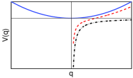
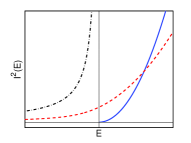
Figure 1: Sketch of the potentials and the corresponding squared action $I^{2}(E)$, which is a positive, monotonically increasing convex function, satisfying the PR property.

In figure 1 we sketch the behaviour of various potentials and the associated squared action $I^{2}(E)$ as a function of the energy $E$, for which the PR property is satisfied for all $E$.

IV Examples of validity of the PR Conjecture

In this section we give examples of Hamiltonian systems in which the PR Conjecture (III) is explicitly and rigorously satisfied for the entire energy range of the potential $V(q)$.

IV.1 Family of Hamiltonians with homogeneous potential and homogeneous kinetic energy

The Hamiltonian is

$$H(p,q)=\frac{p^{2n}}{2n}+\frac{Aq^{2m}}{2m},\quad A>0,\;m>0,\;n>0,$$ (30)

where $m$ and $n$ are positive integers. The action is

$$I\left(E\right) = \frac{1}{2\pi}\oint p\;dq=\frac{1}{\pi}\int_{-q_{0}}^{q_{0}}\sqrt[2n]{2n\left(E-\frac{Aq^{2m}}{2m}\right)}\;dq=$$ (31)

$$= \frac{2^{\frac{2nm+m+n}{2mn}}n^{\frac{1}{2n}}m^{\frac{1}{2m}}}{\pi A^{\frac{1}{2m}}2m}B\left(\frac{1}{2m},\frac{2n+1}{2n}\right)E^{\frac{n+m}{2mn}},$$

where $-q_{0}$ and $q_{0}$ are the turning points, and $B$ is the Beta function,

$$B\left(x,y\right)=\int_{0}^{1}t^{x-1}\left(1-t\right)^{y-1}\;dt.$$

The period $T_{n,m}$ is related to the frequency $\omega_{n,m}$, as $T_{n,m}=\frac{2\pi}{\omega_{n,m}}$. The frequency is

$$\omega_{n,m}\left(E\right)=\frac{\mathrm{d}E}{\mathrm{d}I}=\left(\frac{\mathrm{d}I}{\mathrm{d}E}\right)^{-1},$$

$$\frac{dI}{dE}=a(m,n)\;B\left(\frac{1}{2m},\frac{2n+1}{2n}\right)\,E^{\frac{n+m-2mn}{2mn}},$$ (32)

$$a(m,n)=\frac{2^{\frac{m+n-2mn}{2mn}}n^{\frac{1}{2n}}m^{\frac{1-4m}{2m}}\left(n+m\right)}{\pi A^{\frac{1}{2m}}}$$

Now we calculate the average energy after the kick, denoting the kinetic energy as $K=\frac{p^{2n}}{2n}$,

$$\langle E_{1}\rangle = \langle K\rangle+\langle V_{1}=\rangle\rangle$$ (33)

$$= \langle K\rangle+\langle V_{0}\rangle-\langle V_{0}\rangle+\langle V_{1}\rangle$$

$$= E_{0}+\frac{A_{1}-A_{0}}{A_{0}}\langle V_{0}\rangle.$$

We use the virial theorem Landau and Lifshtz (1969) for this system, rather than equation (8), because the kinetic energy $K=\frac{p^{2n}}{2n}$, $n\geq 1$, is more general than quadratic $n=1$ (and this is the only system in this paper in which we have general nonquadratic kinetic energy), and obtain

$$\langle K\rangle=\frac{m}{n}\langle V_{0}\rangle\Rightarrow\langle V_{0}\rangle=\frac{n}{m+n}E_{0}.$$ (34)

The ratio of the actions is

$$\frac{I\left(\langle E_{1}\rangle\right)}{I(E_{0})}=\frac{\left(1+\left(x-1\right)\frac{n}{n+m}\right)^{\frac{m+n}{2mn}}}{x^{\frac{1}{2m}}}=F_{n,m}(x).$$ (35)

The function $F_{n,m}(x)$ has only one minimum at $x=1$ and the value of the function is equal to $F_{n,m}(1)=1$, as stated by the PR Conjecture.

IV.2 Pendulum

The Hamiltonian is

$$H(q,p)=\frac{p^{2}}{2}-\Omega^{2}\cos q.$$ (36)

The action is

$$I\left(E\right)=\frac{1}{2\pi}\oint p\;dq=\frac{1}{\pi}\int_{-q_{0}}^{q_{0}}\sqrt{2\left(E+\Omega^{2}\cos q\right)}\;dq,$$ (37)

where $-q_{0}$ and $+q_{0}$ are the two turning points in the case of libration (oscillation), defined by $E+\Omega^{2}\cos q_{0}=0$. The action depends on the region in the phase space that we consider. There are three regions of energy $E$ and $q_{0}$ as follows:

1. outside the separatrix, $E>\Omega^{2}$, $q_{0}=\pi$,

2. on the separatrix, $E=\Omega^{2}$, $q_{0}=\pi$

3. inside the separatrix, $E<\Omega^{2}$, $q_{0}<\pi$.

We denote $k=\sqrt{\frac{E+\Omega^{2}}{2\Omega^{2}}}$, and obtain

$$I\left(E\right)=\frac{4}{\pi}\sqrt{2(E+\Omega^{2})}\int_{0}^{\frac{q_{0}}{2}}\sqrt{1-\frac{\sin^{2}\phi}{k^{2}}}\;d\phi.$$ (38)

For the first case, $k\geq 1$, we have

$$I\left(E\right)=\frac{8\Omega k}{\pi}\rm{E}\left(\frac{1}{k}\right),$$ (39)

where $\rm{E}$ is complete elliptic integral of the second kind, which is defined as

$${\rm{E}}\left(k\right)=\int_{0}^{\frac{\pi}{2}}\sqrt{1-k^{2}\sin^{2}\theta}\;d\theta.$$ (40)

For the second case, $k=1$, we have, $I\left(E\right)=\frac{8\Omega}{\pi}$. For the last case, $k\leq 1$, we have

$$I\left(E\right)=\frac{8\Omega}{\pi}\left[{\rm{E}}\left(k\right)-(1-k^{2}){\rm{K}}\left(k\right)\right],$$ (41)

where $\rm{E}$ is the same complete elliptic integral of the second kind and the $\rm{K}$ is elliptic integral of the first kind, which is defined as

$${\rm{K}}\left(k\right)=\int_{0}^{\frac{\pi}{2}}\frac{d\theta}{\sqrt{1-k^{2}\sin^{2}\theta}}.$$

The period $T(E)$ is related to the frequency $\omega(E)$ as $T=\frac{2\pi}{\omega}$, and the frequency is

$$\omega\left(E\right)=\frac{\mathrm{d}E}{\mathrm{d}I}=\left(\frac{\mathrm{d}I}{\mathrm{d}E}\right)^{-1}=\frac{\pi\Omega}{2}\times\left\{\begin{array}[]{lr}\frac{k}{{\rm{K}}\left(\frac{1}{k}\right)},&\mbox{}k\in(1,\infty)\\ \frac{1}{{\rm{K}}\left(k\right)},&\mbox{}k\in[0,1]\\ \end{array}\right.$$

For the average energy we also have two cases. For outside the separatrix, $E_{0}\geq\Omega_{0}^{2}$, we get

$$\langle E_{1}\rangle =E_{0}x+\frac{2\Omega_{0}^{2}\;k_{0}\;{\rm{E}}\left(\frac{1}{k_{0}}\right)}{{\rm{K}}\left(\frac{1}{k_{0}}\right)}(1-x),$$ (42)

whilst for inside the separatrix, $E_{0}\leq\Omega_{0}^{2}$, we have

$$\langle E_{1}\rangle=E_{0}x+2\Omega_{0}^{2}\left[\frac{\rm{E}(k_{0})}{\rm{K}(k_{0})}-\left(1-k_{0}^{2}\right)\right](1-x),$$ (43)

where $k_{0}=\sqrt{\frac{E_{0}^{2}+\Omega_{0}^{2}}{2\Omega_{0}^{2}}}$. We have calculated the average energy $\langle E_{1}\rangle$ from the previous equations, but also checked it numerically. We find that the difference is of the order of about $10^{-13}$. In figure 2 we show the action ratio for the pendulum in the libration regime.

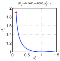
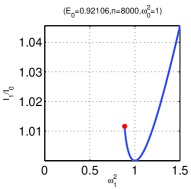
Figure 2: Ratio of initial and final actions for the pendulum, inside the separatrix, with $E_{0}$ is the initial energy and $n$ is the number of the points of initial contour. The bullet is the point $(x_{sep},I(x_{sep}))$, which corresponds to the crossing the separatrix after the kick.

For the case of libration the action $I(E)$ as a power series of $\epsilon=E+\Omega^{2}$ reads as

$$I(E) =\frac{\epsilon}{4194304\Omega^{11}}(1323\;\epsilon^{5}+3920\Omega^{2}\;\epsilon^{4}+12800\Omega^{4}\;\epsilon^{3}$$

$$+49152\Omega^{6}\;\epsilon^{2}+262144\Omega^{8}\;\epsilon+4194304\Omega^{10}+h.o.t.).$$

and the function $I^{2}(E)$ is plotted in figure 3. The PR property is satisfied.

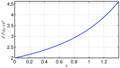
Figure 3: The pendulum: The second derivative $d^{2}I^{2}(E)/dE^{2}$, with $\omega=1$.

IV.3 Radial Kepler problem with zero angular momentum

The Hamiltonian is

$$H(r,p)=\frac{p^{2}}{2}-\frac{A}{r},\quad A>0.$$ (45)

The action is

$$I\left(E\right) = \frac{1}{2\pi}\oint p\;dr=$$ (46)

$$= \frac{1}{\pi}\int_{r_{1}}^{r_{2}}\sqrt{2\left(E+\frac{A}{r}\right)}\;dr=\frac{A}{\sqrt{2|E|}},$$

where $r_{1}$ and $r_{2}$ are the two turning points. In fact, $r_{1}=0$. The period $T$ is related to the frequency $\omega$, as $T=\frac{2\pi}{\omega}$,

$$\omega\left(E\right)=\frac{\mathrm{d}E}{\mathrm{d}I}=\left(\frac{\mathrm{d}I}{\mathrm{d}E}\right)^{-1}=\frac{2\sqrt{2}\;|E|^{\frac{3}{2}}}{A}.$$ (47)

The average energy is

$$\langle E_{1}\rangle=\langle K\rangle+\langle V_{1}\rangle=E_{0}+\frac{A_{1}-A_{0}}{A_{0}}\langle V_{0}\rangle.$$

We can use the virial theorem Landau and Lifshtz (1969) to calculate the average potential,

$$\langle E_{0}\rangle=\frac{\langle V_{0}\rangle}{2}=E_{0}.$$ (48)

Finally, we get the ratio of the actions $I_{1}$ and $I_{0}$

$$\frac{I\left(\langle E_{1}\rangle\right)}{I(E_{0})}=\frac{x}{\sqrt{2x-1}}=F(x),$$ (49)

where $x=A_{1}/A_{0}$. For this Kepler problem we have positive average energy $\langle E_{1}\rangle$ if $A_{1}\leq A_{0}/2$. Thus the ratio of the actions $I_{1}\geq I_{0}$, for no-escape orbits, as the function $F(x)$ has the minimum at $x=1$ and the value of the function is $F(1)=1$ in accordance with the PR Conjecture.

IV.4 Radial Kepler problem with nonzero angular momentum

The Hamiltonian with the angular momentum $M$ is

$$H(r,p)=\frac{p^{2}}{2}-A\left(\frac{a}{r}-\frac{M^{2}}{2r^{2}}\right),\quad A>0,\;a>0,\;M^{2}>0.$$ (50)

The action is

$$I\left(E\right) = \frac{1}{2\pi}\oint p\;dq=\frac{1}{\pi}\int_{r_{1}}^{r_{2}}\sqrt{2\left(E+A\left(\frac{a}{r}-\frac{M^{2}}{2r^{2}}\right)\right)}\;dr\Rightarrow$$

$$I\left(E\right) = \frac{A\;a}{\sqrt{2|E|}}-\sqrt{A}\;M.$$ (51)

Here $r_{1}$ and $r_{2}$ are the two turning points. The frequency is

$$\omega\left(E\right)=\frac{\mathrm{d}E}{\mathrm{d}I}=\left(\frac{\mathrm{d}I}{\mathrm{d}E}\right)^{-1}=\frac{2\sqrt{2}\;|E|^{\frac{3}{2}}}{A\;a}.$$ (52)

The average energy is, using equation (8),

$$\langle E_{1}\rangle=E_{0}x+\frac{\sqrt{2}\;|E_{0}|^{\frac{3}{2}}}{A_{0}\;a}\left(\frac{A_{0}\;a}{\sqrt{2\;|E_{0}|}}-\sqrt{A_{0}}\;M\right)(1-x),$$ (53)

where $x=A_{1}/A_{0}$.
We have positive average energy after the kick, if

$$x\leq x_{esc}=\frac{A_{0}\;a-\sqrt{2A_{0}}\;M|E_{0}|^{\frac{1}{2}}}{2A_{0}\;a-\sqrt{2A_{0}}\;M|E_{0}|^{\frac{1}{2}}}.$$

For the action ratio we have finally

$$\frac{I\left(\langle E_{1}\rangle\right)}{I\left(E_{0}\right)}=\frac{x\sqrt{\frac{1}{2x-1+(1-x)c}}-c\sqrt{x}}{1-c}=F(x),$$ (54)

where $c=\frac{M\sqrt{2|E_{0}|}}{a\sqrt{A_{0}}}$. Since the minimal energy $E_{min}\leq 0$ is determined by the condition $I(E_{min})=0$, we find from (IV.4) $|E_{min}|=a^{2}A/(2M^{2})$, and thus due to $|E_{0}|\leq E_{min}$ we have $c\leq 1$. If $M=0$ and consequently $c=0$, we recover the result for the Kepler problem with zero angular momentum of the previous subsection IV.3. The derivative of $F(x)$ is

$$\frac{\partial F(x)}{\partial x}=\frac{-\frac{x}{2}(2-c)\left(\frac{1}{B(x)}\right)^{\frac{3}{2}}+\left(\frac{1}{B(x)}\right)^{\frac{1}{2}}-\frac{c}{2\sqrt{x}}}{1-c},$$ (55)

where $B(x)=(2-c)x+c-1$. There is only one root for $\frac{\partial F(x)}{\partial x}=0$, namely precisely $x=1$. For the second derivative of $F(x)$ we find

$$\frac{\partial^{2}F(x)}{\partial x^{2}}=\frac{\frac{3}{4}(c-2)^{2}x\left(\frac{1}{B(x)}\right)^{\frac{5}{2}}+(c-2)\left(\frac{1}{B(x)}\right)^{\frac{3}{2}}+\frac{c}{4x^{3/2}}}{1-c},$$ (56)

and at $x=1$ we have

$$\frac{\partial^{2}F(x)}{\partial x^{2}}|_{x=1}=1-\frac{3}{4}c>0$$ (57)

for all $c\leq 1$. Thus there is only one minimum for the function $F(x)$ at $x=1$, with $F(1)=1$, exactly in accordance with the PR Conjecture. In figure 4 we show the action ratio as a function of $x$ for $c=1/2$.

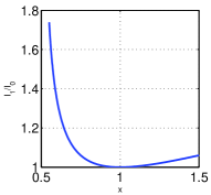
Figure 4: Action ratio for the Kepler potential with nonzero angular momentum, with $A_{0}=1$ and $c=\frac{1}{2}$. The $x$ for escape orbit is $x\leq x_{esc}=\frac{1}{3}$, with action ratio $I_{1}/I_{0}\rightarrow\infty$ as $x\rightarrow x_{esc}$.

IV.5 Morse potential

The Hamiltonian is

$$H(q,p)=\frac{p^{2}}{2}+A(e^{-2\lambda r}-e^{-\lambda r}),\quad A>0,\quad\lambda>0.$$ (58)

The minimum of the potential is equal to $-A/4$. The action is

$$I\left(E\right)=\frac{1}{2\pi}\oint p\;dr=\frac{1}{\pi}\int_{r_{1}}^{r_{2}}\sqrt{2\left(E-A(e^{-2\lambda r}-e^{-\lambda r})\right)}\;dr,$$

where $r_{1}$ and $r_{2}$ are the two turning points, and we get

$$I\left(E\right)=-\frac{\sqrt{2|E|}}{\lambda}+\frac{\sqrt{A}}{\lambda\sqrt{2}}.$$ (59)

The frequency $\omega$ is

$$\omega\left(E\right)=\frac{\mathrm{d}E}{\mathrm{d}I}=\left(\frac{\mathrm{d}I}{\mathrm{d}E}\right)^{-1}=\lambda\sqrt{2|E|}.$$ (60)

For the average energy, we have

$$\langle E_{1}\rangle=\langle K\rangle+\langle V_{1}\rangle=E_{0}+\frac{A_{1}-A_{0}}{A_{0}}\langle V_{0}\rangle.$$

In contradistinction to some other systems, here we can find the $r$ as a function of time $t$ in an explicit closed form

$$\frac{dr}{dt}=\sqrt{2(E-A(e^{-\lambda r}-e^{-2\lambda r}))}\Rightarrow$$ (61)

$$t=\int\frac{dr}{\sqrt{2(E-A(e^{-\lambda r}-e^{-2\lambda r}))}}.$$

Using $u=e^{-\lambda r}$ and after some calculations we obtain

$$t=-\frac{\arcsin\left(\frac{2E+Au}{u\sqrt{4AE+A^{2}}}\right)}{\lambda\sqrt{2|E|}},$$ (62)

or,

$$r(t)=-\frac{1}{\lambda}\ln\left[\frac{2|E|}{\sqrt{4EA+A^{2}}\;\sin\left(\sqrt{2|E|}\;\lambda t\right)+A}\right].$$ (63)

Finally the average energy is, either using the equation (8) or doing the direct averaging over time using (63),

$$\langle E_{1}\rangle=E_{0}+\frac{\sqrt{A_{0}|E_{0}|}}{2}(1-x),$$ (64)

where $x=A_{1}/A_{0}$. We have positive average energy after the kick, at $x\leq x_{esc}=1-2|E_{0}|/A_{0}$. For the action ratio we have

$$\frac{I\left(\langle E_{1}\rangle\right)}{I\left(E_{0}\right)}=\frac{\sqrt{x}-2\sqrt{|\frac{E_{0}}{A_{0}}+\frac{1}{2}\sqrt{\frac{|E_{0}|}{A_{0}}}\;(1-x)|}}{1-2\sqrt{\frac{|E_{0}|}{A_{0}}}}=F(x).$$ (65)

We define $E_{0}=-A_{0}/4+\epsilon$, $0\leq\epsilon\leq A_{0}/4$, and $c=\epsilon/A_{0}$, so that $0\leq c\leq 1/4$, and simplify

$$F(x)=\frac{I\left(\langle E_{1}\rangle\right)}{I\left(E_{0}\right)}=\frac{\sqrt{x}-2\sqrt{|-c+\frac{1}{4}+\frac{\sqrt{-c+\frac{1}{4}}}{2}\;(1-x)|}}{1-2\sqrt{|\frac{1}{4}-c|}}.$$ (66)

The function $F(x)$ has a single minimum at $x=1$ and $F(1)=1$, in agreement with the PR Conjecture. In figure 5 we plot the action ratio as a function of $A_{1}$ at $\lambda=1$ and $A_{0}=1$

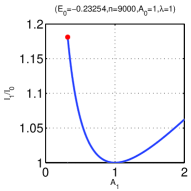
Figure 5: Action ratio for the Morse potential, with $\lambda=1$. $A_{0}=1$ and $n$ is the number of points in initial contour. $x$ for escape orbits is $x\leq x_{esc}=0.31803$, with the action ratio $I_{1}/I_{0}=1.18103$, marked by a bullet.

IV.6 Pöschl-Teller I potential

The Hamiltonian is

$$H(q,p)=\frac{p^{2}}{2}+\frac{A}{\cos^{2}\left(\lambda q\right)},\quad\lambda>0,\;A>0.$$ (67)

The action is

$$I\left(E\right) =\frac{1}{2\pi}\oint p\;dq=\frac{1}{\pi}\int_{q_{1}}^{q_{2}}\sqrt{2\left(E-\frac{A}{\cos^{2}\lambda q}\right)}\;dq,$$

where $q_{1}$ and $q_{2}$ are the two turning points. Using transformation, $y=\tan\left(\lambda q\right)$ and after calculation, we get finally,

$$I\left(E\right)=\frac{\sqrt{2}}{\lambda}(\sqrt{E}-\sqrt{A}).$$ (68)

The frequency is

$$\omega\left(E\right)=\frac{\mathrm{d}E}{\mathrm{d}I}=\left(\frac{\mathrm{d}I}{\mathrm{d}E}\right)^{-1}=\lambda\sqrt{2E}.$$ (69)

Now we calculate the final average energy either using (8) or by direct averaging

$$\langle E_{1}\rangle=E_{0}+\frac{A_{1}-A_{0}}{A_{0}}\langle V_{0}\rangle.$$

where

$$\langle V_{0}\rangle=\frac{1}{T}\int_{0}^{T}\frac{A_{0}}{\cos^{2}\left(\lambda q(t)\right)}\;dt.$$ (70)

Here again we can express $q$ as function of time $t$, namely, after some straightforward calculation, we obtain

$$q(t)=\frac{1}{\lambda}\arcsin\left(\sqrt{\frac{E-A}{E}}\sin\left(\lambda t\sqrt{2E}\right)\right).$$ (71)

Further, using the transformation $y=\lambda\sqrt{2E_{0}}t$, we find

$$\langle V_{0}\rangle = \frac{1}{T}\int_{0}^{T}\frac{A_{0}}{\cos^{2}\left(\lambda q(t)\right)}\;dt$$

$$= \frac{A_{0}}{\lambda T\sqrt{2E_{0}}}\int_{0}^{2\pi}\frac{dy}{1-\frac{E_{0}-A_{0}}{E_{0}}\sin^{2}y}\Rightarrow$$

$$\langle V_{0}\rangle = \sqrt{A_{0}E_{0}}.$$ (72)

The average energy, with $x=A_{1}/A_{0}$, is thus

$$\langle E_{1}\rangle=E_{0}+(x-1)\sqrt{E_{0}A_{0}}.$$ (73)

The minimum energy is at $E_{0}=A_{0}$, so we write $E_{0}=A_{0}+\epsilon$, where $\epsilon\geq 0$. Then, setting $c=\epsilon/A_{0}$, we obtain the action ratio $F(x)$ as

$$\frac{I\left(\langle E_{1}\rangle\right)}{I\left(E_{0}\right)}=F(x)=\frac{\sqrt{c+1+\sqrt{c+1}(x-1)}-\sqrt{x}}{\sqrt{c+1}-1}.$$ (74)

This function $F(x)$ has a single minimum at $x=1$ and $F(1)=1$, in agreement with the PR Conjecture.

IV.7 Pöschl-Teller II potential

The Hamiltonian is

$$H(q,p)=\frac{p^{2}}{2}-\frac{A}{\cosh^{2}\left(\lambda q\right)},\quad\lambda>0,\;A>0.$$ (75)

The action is

$$I\left(E\right) =\frac{1}{2\pi}\oint p\;dq=\frac{\sqrt{2}}{\lambda}\left(\sqrt{A}-\sqrt{|E|}\right).$$ (76)

The frequency is

$$\omega\left(E\right)=\frac{\mathrm{d}E}{\mathrm{d}I}=\left(\frac{\mathrm{d}I}{\mathrm{d}E}\right)^{-1}=\lambda\sqrt{2|E|}.$$ (77)

The final average energy is

$$\langle E_{1}\rangle =\langle K\rangle+\langle V_{1}\rangle=\langle K\rangle+\langle V_{0}\rangle-\langle V_{0}\rangle+\langle V_{1}\rangle\Leftrightarrow$$

$$\langle E_{1}\rangle =E_{0}+\frac{A_{1}-A_{0}}{A_{0}}\langle V_{0}\rangle,$$

where we need

$$\langle V_{0}\rangle=\frac{1}{T}\int_{0}^{T}\frac{A_{0}}{\cosh^{2}\left(\lambda q(t)\right)}\;dt.$$ (78)

In this case again we can find the explicit solution of $q(t)$ in a closed form, namely

$$q(t)=\frac{1}{\lambda}\rm{arcsinh}\left(\sqrt{\frac{E+A}{|E|}}\sin\left(\lambda t\sqrt{2|E|}\right)\right).$$ (79)

The average potential is

$$\langle V_{0}\rangle = -\frac{1}{T}\int_{0}^{T}\frac{A_{0}}{\cosh^{2}\left(\lambda q(t)\right)}\;dt$$

$$= -\frac{A_{0}}{\lambda T\sqrt{2|E_{0}|}}\int_{0}^{2\pi}\frac{dy}{1+\frac{E_{0}+A_{0}}{|E_{0}|}\sinh^{2}y}\Rightarrow$$

$$\langle V_{0}\rangle = -\sqrt{A_{0}|E_{0}|},$$ (80)

The minimum of the potential is $-A_{0}$, so we introduce $\epsilon$, such that $E_{0}=-A_{0}+\epsilon$. Further, by defining $c=\epsilon/A_{0}$, we can calculate the ratio of the actions after the kick, as follows

$$\frac{I\left(\langle E_{1}\rangle\right)}{I\left(E_{0}\right)}=F(x)=\frac{\sqrt{|c-1+\sqrt{|c-1|}(x-1)|}-\sqrt{x}}{\sqrt{|c-1|}-1}.$$ (81)

We have positive average energy after the kick if $x\leq x_{esc}=1-\sqrt{|E_{0}|/A_{0}}$. For $x\geq x_{esc}$ the function $F(x)$ has a single minimum at $x=1$ and its value is $F(1)=1$, in complete agreement with the PR Conjecture.

IV.8 Cosh potential

The Hamiltonian is

$$H(q,p)=\frac{p^{2}}{2}+A\cosh\lambda q,\quad A>0.$$ (82)

The action is

$$I(E) = -\frac{i\,4\sqrt{2(E-A)}}{\pi\lambda}$$ (83)

$$\quad\,{\rm E}\left(\frac{i}{2}\log\left(\frac{E+\sqrt{E^{2}+A^{2}}}{A}\right),\frac{2A}{A-E}\right),$$

where ${\rm E}$ is the elliptic integral of the second kind, with $k^{2}=2A/(A-E)$, and the definition

$${\rm E}(\phi,k)=\int_{0}^{\phi}dt\sqrt{1-k^{2}\sin^{2}t}.$$ (84)

For large energies $E\gg A$ we have the asymptotics $I(E)\approx\sqrt{E}\log E$, and the second derivative of $I^{2}$ is approximately

$$\frac{\partial^{2}I^{2}(E)}{\partial E^{2}}\propto\frac{2\log E}{E},$$ (85)

which means again that the PR Conjecture is satisfied. In figure 6 we plot the function $I^{2}(E)$ as a function of $E$ for the case $A=0$ and $\lambda=0$.

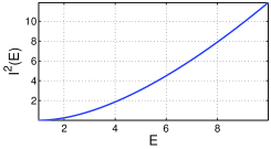
Figure 6: Cosh potential: $I^{2}(E)$ as a function of $E$, for $A=1$ and $\lambda=1$, showing that it is a convex function, satisfying the PR property.

V Studies of breaking the PR Conjecture

In this section we shall investigate the potentials where the PR Conjecture is violated, either because of the nonanalyticity (nonsmoothness) or due to the closeness to a stationary point (separatrix in the phase space). Since the PR Conjecture in full generality is not true, we will better speak of the PR property rather than PR Conjecture. We shall show the breaking of the PR property in case of $C^{0}$ potential in the subsection V.1, and then demonstrate in the two next subsections that PR property is restored if the first derivative is continuous, and even more so if the second derivative of the potential $V(q)$ is continuous. After that we shall study what happens if the potential is not a single well potential, but has other stationary points, implying the existence of a separatrix in the phase space. In those cases the PR property can be broken, typically for a certain energy range around the separatrix.

V.1 Harmonic oscillator in a box

The first example of a potential (system) which violates the PR Conjecture is a nonanalytic potential, namely the harmonic oscillator in a box. The Hamiltonian is

$$H(q,p)=\frac{p^{2}}{2}+V(q),$$ (86)

where

$$V(q)=\left\{\begin{array}[]{lr}\frac{\omega^{2}q^{2}}{2},&\mbox{}q\in[-q_{0},q_{0}]\\ q=\infty,&\mbox{}|q|\geq q_{0}\end{array}\right\},$$

and the kick parameter is $A=-\omega^{2}$. The potential is continuous, but has discontinuous first derivative at $q=q_{0}$, so it is $C^{0}$ only. For the energy $E$ smaller than $E_{c}=\omega^{2}q_{0}^{2}/2$ the system behaves just as the ordinary linear oscillator treated in subsection IV.1, equation (97), and $d^{2}I^{2}/dE^{2}=1/\omega^{2}\geq 0$, whilst at $E\geq E_{c}$ the box potential plays a role. For a pure box potential without the harmonic oscillator we have $I\propto\sqrt{E}$ and consequently $d^{2}I^{2}/dE^{2}=0$. As we will see, for the combined potential (107) at $E\geq E_{c}$ we find that $d^{2}I^{2}/dE^{2}<0$. The action at $E\geq E_{c}$ is

$$I\left(E\right) =\frac{1}{2\pi}\oint p\;dq=\frac{1}{\pi}\int_{-q_{0}}^{q_{0}}\sqrt{2\left(E+\frac{1}{2}\omega^{2}q^{2}\right)}\;dq.$$

$$I\left(E\right) =\frac{2E}{\pi\omega}\left({\rm{arcsin}}\left(\frac{q_{0}\omega}{\sqrt{2E}}\right)+\frac{q_{0}\omega}{\sqrt{2E}}\sqrt{1-\frac{q_{0}^{2}\omega^{2}}{2E}}\;\right).$$ (87)

The action in series expansion is

$$I(E)=\frac{4Ex_{0}}{\pi\omega}\left(1-\frac{x_{0}^{2}}{6}+\frac{3x_{0}^{4}}{20}-\frac{x_{0}^{6}}{112}+h.o.t.\right)$$ (88)

where $x_{0}=\frac{q_{0}\omega}{\sqrt{2E}}$. Finally, we have

$$\frac{\partial^{2}I^{2}(E)}{\partial E^{2}}=-\frac{16x_{0}^{6}}{45\pi^{2}\omega^{2}}\left(2+\frac{18}{7}x_{0}^{2}+h.o.t.\right)\leq 0$$ (89)

Thus we see that due to the harmonic potential inside the box $d^{2}I^{2}/dE^{2}$ is no longer zero, but negative. Therefore, the curve $I^{2}(E)$ is not convex for the energy range $E\geq E_{c}=\omega^{2}q_{0}^{2}/2$ and implies that $Q$ defined in equation (18) and given in the closed form in (25), is negative and therefore $F(x)$ has a maximum $F(1)=1$ at $x=1$ instead of a minimum, which is a violation of the PR property at energy range $E\geq E_{c}$.

V.2 Quadratic-linear potential

The previous nonanalytic potential does not possess the PR property, due to nonanalyticity. In fac, $V(q)$ is only a continuous function, the first derivative is discontinuous. Therefore, let us look at an example where the first derivative is smooth, whilst the second is not. Thus we construct a potential which is quadratic (harmonic) up to $|q|\leq q_{0}$, and linear outside the interval $(-q_{0},q_{0})$, such that the first derivative $dV/dq$ at $|q|=q_{0}$ is continuous. The Hamiltonian is

$$H(q,p)=\frac{p^{2}}{2}-A\;f(q),\quad A>0.$$ (90)

where

$$f(q)=\left\{\begin{array}[]{lr}-\frac{\omega^{2}q^{2}}{2},&\mbox{}q\in[-q_{0},q_{0}]\\ -\omega^{2}q_{0}|q|+\frac{\omega^{2}q_{0}^{2}}{2},&\mbox{}q\not\in[-q_{0},q_{0}].\end{array}\right.$$

In figure 7 we show the plot of the $I^{2}(E)$, obtained numerically, and it is obvious that it is a convex function for all $E$, meaning that the PR property is satisfied. We might conjecture that the $C^{1}$ smoothness of a single minimum potential $V(q)=-Af(q)$ is enough for the PR property to hold.

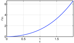
Figure 7: Quadratic-linear potential. The $I^{2}(E)$ with $A=1$, $\omega=1$ and $q_{0}=1$.

V.3 Quadratic-quartic potential

Let us increase the degree of smoothness and consider the $V(q)$ functions of class $C^{2}$, i.e. having a continuous second derivative only. Of course, we expect the PR property to hold, and this is indeed observed. The Hamiltonian is

$$H(q,p)=\frac{p^{2}}{2}-A\;f(q),\quad A>0,$$ (91)

where

$$f(q)=\left\{\begin{array}[]{lr}-\frac{\omega^{2}q^{2}}{2},&\mbox{}q\in[-q_{0},q_{0}]\\ -\frac{\omega^{2}(q+2q_{0}\;{\rm sign}(q))^{4}}{108\;q_{0}^{2}}+\frac{\omega^{2}q_{0}^{2}}{4},&\mbox{}q\not\in[-q_{0},q_{0}].\end{array}\right.$$

We have calculated $I(E)$ numerically, and show the plot of the function $I^{2}(E)$ in figure 8 and it is obvious that it is a convex function of $E$ for all $E$. Thus, the PR property is satisfied.

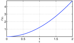
Figure 8: Quadratic-quartic potential: $I^{2}(E)$ with $A=1$, $\omega=1$ and $q_{0}=1$.

V.4 Sextic potential

The Hamiltonian is

$$H(q,p)=\frac{p^{2}}{2}-A\;f(q),\quad A>0,$$ (92)

where the potential $V(q)=-Af(q)$ is given by

$$f(q)=-(cq+(q-1)^{3})(cq+(q+1)^{3}),\;c\geq 0.$$ (93)

This model cannot be analyzed analytically. If $c=0$, there are two stationary points at $q=\pm 1$, namely inflection points, at the energy (potential level) $E=V=0$. By numerical techniques one can convince himself that the $dI^{2}/dE^{2}$ can be negative if the energy is close to the value of the stationary points. This is still true if $c$ is nonzero, but small. We choose $c=0.001$. The potential is plotted in figure 9, and it has only one minimum.

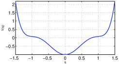
Figure 9: Sextic potential, with $A=1$, $c=0.001$, for $-1.5\leq q\leq 1.5$.

Now let us calculate directly the action ratio $I_{1}/I_{0}=F(x)$ for the parameters $A_{0}=1$ as a function of $x=A_{1}$. We observe three cases in figure 10. At high energy $E=1.9584$ there is a minimum of $F(x)$ at $x=1$, which means that the PR property is satisfied. At small energy $E=0.032004$ we have a maximum at $x=1$, meaning the violation of the PR property, whilst at some intermediate energy $E=0.10509$ we have a very flat maximum, very close to an inflection point.

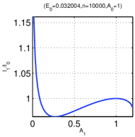
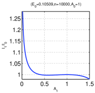
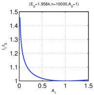
Figure 10: Sextic potential. The action ratio $I_{1}/I_{0}$ with $A_{0}=1$, $c=0.001$ and initial energy $E_{0}$. $n$ is the number of the points in the initial ensemble. Clockwise: For (a) we find a maximum, (b) inflection point (or very shallow maximum) and in (c) we have a minimum, at $x=A_{1}/A_{0}=1$. Only in the last case (c) PR property is satisfied.

V.5 Quartic double well potential

The Hamiltonian is

$$H(q,p)=\frac{p^{2}}{2}-A\;f(q),\quad A>0,$$ (94)

where the quartic double well potential is

$$V(q)=-Af(q)=A(q-1)^{2}(q+1)^{2}.$$ (95)

We plot it in figure 11.

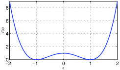
Figure 11: Quartic double well potential, with $A=1$, for $-2\leq q\leq 2$.

We start above the potential maximum $E_{0}>A_{0}$, and make a kick $A_{0}\rightarrow A_{1}$. The critical value $x_{c}$ of $x=A_{1}/A_{0}$ for the energy level $\langle E_{1}\rangle$ to stay outside the separatrix at $E=A_{1}$, namely $x\leq x_{c}$, is

$$x_{c}=\frac{\pi I_{0}}{\pi I_{0}+A_{1}T_{0}-E_{0}T_{0}}.$$ (96)

We have calculated the action ratio $I_{1}/I_{0}$, assuming $A_{0}=1$, as a function of $x=A_{1}$ using only numerical methods, and we find three different cases for the point $x=1$ in figure 12. For the energy $E=1.0323$ close to the potential local maximum having level $V=1$ at $q=0$ we find a maximum of $F(x)$ at $x=1$, meaning the broken PR property, whilst at high energy $E=5.0226$ we observe a local minimum at $x=1$, meaning that the PR Property is satisfied. At intermediate energy $E=1.2205$ we are close to an inflection point.

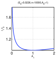
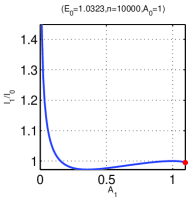
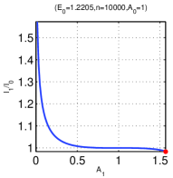
Figure 12: Quartic double well potential: The action ratio $I_{1}/I_{0}$ with $A_{0}=1$ and initial energy $E_{0}$ as a function of $x=A_{1}$. $n$ is the number of points in the initial ensemble and the bullet denotes the critical point at which we cross the separatrix becoming trapped in one of the two wells. Observe the behaviour at $A_{1}=1$, clockwise: For (a) we find a minimum, in (b) we have a maximum, and in (c) the inflection point.

The examples of this section demonstrate that the PR property can be broken if the potential has a single minimum but is not sufficiently smooth (if it is just $C^{0}$), whilst the class $C^{1}$ or higher is sufficient for the PR property to hold. On the other hand, if the potential is analytic but is not a single minimum potential, thus having a separatrix in the phase space, the PR property can be broken for energies in the range near to the separatrix energy level. Moreover, the potential can be analytic, with a single minimum, but has a region where there is almost an inflection point, where the breaking of PR property is observed for the energies in the range close to the almost-inflection point.

VI Discussion and conclusions

In this work we have analyzed the statistical properties of one degree of freedom parametrically kicked Hamiltonian systems, which is the extreme case of fast time dependence, being the opposite extreme to an adiabatic, infinitely slow, changing. As such, the parametric kick behaviour is a very good approximation for the behaviour of the systems under very fast changes in the system parameters, within a time scale of less than one period of oscillation, as has been demonstrated already by Papamikos and Robnik Papamikos and Robnik (2011). The most natural ensemble, and the most important one is the microcanonical ensemble, because if we have a large ensemble of identical systems with the same (”prepared”) energy, and we do not have any further information about them, the uniform distribution with respect to the canonical angle (”the phases”) is the most appropriate one. Our main interest is in the value of the final average energy, just after the parametric kick, and the value of the action, identical to the adiabatic invariant, or identical to the area $\Omega$ inside the energy contour (divided by $2\pi$) in the phase space. If the value of the adiabatic invariant at the average final energy increases after the kick, we say that the system has the PR property, following the conjecture put forward by Papamikos and Robnik Papamikos and Robnik (2011). As discussed in section 2 this implies increasing Gibbs entropy $S_{G}$ at the mean energy.

It turns out that the PR property is satisfied in a vast variety of potentials in which we have proven the validity of the conjecture by direct and rigorous calculations. However, the PR Conjecture is not always satisfied. We have explored exceptions and found that the PR property can be broken if the potential is not sufficiently smooth (if it is $C^{0}$ only), or if it has several local minima and maxima, implying existence of a separatrix, or of several separatrices, in the phase space. Of course, these complications are not unexpected, because the existence of a separatrix in the phase space always plays and important role, e.g. crossing a separatrix breaks the validity of the adiabatic theorem Arnold (1989). In energy ranges close to the separatrix, i.e. stationary points of the potential, the PR property can be broken. Further study of the PR properties in Hamiltonian systems with one and also with more degrees of freedom seems to be very challenging and important. Our results suggest that the following proposition might be true: A strictly convex $C^{2}$ potential (thus with a single minimum) has the PR property. A proof of this statement is lacking and left for the future.

We do believe that this research and the results are important in the statistical mechanics of few body systems, and also for the large, macroscopical, ensembles of identical noninteracting parametrically driven nonlinear oscillators, as discussed in section 2. Further theoretical research is in progress. Moreover, the research of the general statistical behaviour of the energy distribution (and of other dynamical variables), in the regimes between the ideal adiabatic variation and the parametric kicking, is of great interest and importance.

Appendix A: Summary of the cases with or without the PR property

Examples of PR property valid for all energies

1. Homogeneous power law kinetic energy and potential

   $$H(p,q)=\frac{p^{2n}}{2n}+\frac{Aq^{2m}}{2m},\quad A>0,\;m>0,\;n>0.$$ (97)

2. Pendulum (for the average energy inside the separatrix - librations)

   $$H(q,p)=\frac{p^{2}}{2}-\Omega^{2}\cos q.$$ (98)

3. Radial Kepler problem with zero angular momentum

   $$H(r,p)=\frac{p^{2}}{2}-\frac{A}{r},\quad A>0.$$ (99)

4. Radial Kepler problem with nonzero angular momentum

   $$H(r,p)=\frac{p^{2}}{2}-A\left(\frac{a}{r}-\frac{M^{2}}{2r^{2}}\right),\quad A>0,\;a>0,\;M^{2}>0.$$ (100)

5. Morse potential

   $$H(q,p)=\frac{p^{2}}{2}+A(e^{-2\lambda r}-e^{-\lambda r}),\quad A>0,\quad\lambda>0.$$ (101)

6. Pöschl-Teller I potential

   $$H(q,p)=\frac{p^{2}}{2}+\frac{A}{\cos^{2}\left(\lambda q\right)},\quad\lambda>0,\;A>0.$$ (102)

7. Pöschl-Teller II potential

   $$H(q,p)=\frac{p^{2}}{2}-\frac{A}{\cosh^{2}\left(\lambda q\right)},\quad\lambda>0,\;A>0.$$ (103)

8. Cosh potential

   $$H(q,p)=\frac{p^{2}}{2}+A\cosh\lambda q,\quad A>0.$$ (104)

9. Quadratic-linear potential $C^{1}$

   $$H(q,p)=\frac{p^{2}}{2}-A\;f(q),\quad A>0,$$ (105)

   where

   $$f(q)=\left\{\begin{array}[]{lr}-\frac{\omega^{2}q^{2}}{2},&\mbox{}q\in[-q_{0},q_{0}]\\ -\omega^{2}q_{0}|q|+\frac{\omega^{2}q_{0}^{2}}{2},&\mbox{}q\not\in[-q_{0},q_{0}].\end{array}\right.$$

10. Quadratic-quartic potential $C^{2}$

    $$H(q,p)=\frac{p^{2}}{2}-A\;f(q),\quad A>0,$$ (106)

    where

    $$f(q)=\left\{\begin{array}[]{lr}-\frac{\omega^{2}q^{2}}{2},&\mbox{}q\in[-q_{0},q_{0}]\\ -\frac{\omega^{2}(q+2q_{0}\;{\rm sign}(q))^{4}}{108\;q_{0}^{2}}+\frac{\omega^{2}q_{0}^{2}}{4},&\mbox{}q\not\in[-q_{0},q_{0}].\end{array}\right.$$

Examples of violated PR property

1. Harmonic oscillator in a box ($C^{0}$, entirely convex, violation at $E\geq V(q_{0})$ )

   $$H(q,p)=\frac{p^{2}}{2}+V(q),$$ (107)

   where

   $$V(q)=\left\{\begin{array}[]{lr}\frac{\omega^{2}q^{2}}{2},&\mbox{}q\in[-q_{0},q_{0}]\\ q=\infty,&\mbox{}|q|\geq q_{0}\end{array}\right..$$

2. Sextic potential (single minimum potential)

   violation around $E=0$, due to the flatness near $|q|\approx 1$ (close to a stationary point)

   $$H(q,p)=\frac{p^{2}}{2}-A\;f(q),\quad A>0,$$ (108)

   where the potential $V(q)=-Af(q)$ is given by

   $$f(q)=-(cq+(q-1)^{3})(cq+(q+1)^{3}),\;c\geq 0.$$

3. Quartic double well potential

   PR property broken near the local maximum $E=A$.

   $$H(q,p)=\frac{p^{2}}{2}-A\;f(q),\quad A>0,$$ (109)

   where the quartic double well potential is

   $$V(q)=-Af(q)=A(q-1)^{2}(q+1)^{2}.$$

References

- Papamikos and Robnik (2011) G. Papamikos and M. Robnik, Journal of Physics A: Mathematical and Theoretical 44, 315102 (2011).
- Robnik and Romanovski (2006a) M. Robnik and V. G. Romanovski, Journal of Physics A: Mathematical and Theoretical 33, L35 (2006a).
- Robnik and Romanovski (2006b) M. Robnik and V. G. Romanovski, Open Systems & Information Dynamics 13, 197 (2006b).
- Robnik et al. (2006) M. Robnik, V. G. Romanovski, and H.-J. Stöckmann, Journal of Physics A: Mathematical and General , L551 (2006).
- Kuzmin and Robnik (2007) A. V. Kuzmin and M. Robnik, Rep. on Math. Phys. 60, 69 (2007).
- Robnik and Romanovski (2008) M. V. Robnik and V. G. Romanovski, in Let’s Face Chaos through Nonlinear Dynamics, AIP Conference Proceedings, Vol. 1076 (AIP, Mellvile, New York, 2008).
- Robnik and Romanovski (2000) M. Robnik and V. G. Romanovski, Journal of Physics A: Mathematical and General 33, 5093 (2000).
- Arnold (1989) V. I. Arnold, Mathematical Methods of Classical Mechanics, 2nd ed. (Springer-Verlag, 1989).
- McLachlan (1995) R. I. McLachlan, SIAM J.Sci.Comput. 16, 151 (1995).
- McLachlan and Quispel (2002) R. I. McLachlan and G. R. W. Quispel, Acta Numerica 11, 341 (2002).
- Hairer et al. (2006) E. Hairer, C. Lubich, and G. Wanner, Geometric Numerical Integration, 2nd ed., Vol. 31 (Springer-Verlag, 2006).
- Leimkuhler and Reich (2004) B. Leimkuhler and S. Reich, Simulating Hamiltonian Dynamics, 1st ed. (Cambridge University Press, 2004).
- Senz-Serna and Calvo (1994) J. M. Senz-Serna and M. P. Calvo, Numerical Hamiltonian Problems (Chapman & Hall, 1994).
- Shimada and Yoshida (1996) M. Shimada and H. Yoshida, Publ. Astron. Soc. Japan 48, 147 (1996).
- Yoshida (1990) H. Yoshida, Phys. Lett. A 150, 263 (1990).
- Yoshida (1993) H. Yoshida, Celestial Mechanics and Dynamical Astronomy 56, 27 (1993).
- Papamikos (2011) G. Papamikos, Analisis of the adiabatic invariants and the statistical properties of time-dependent low-dimensional Hamilton systems, Ph.D. thesis, University of Ljubljana, FMF (2011).
- Robnik (2013) M. Robnik, Lect. Notes in Comp. Sci. (2013).
- Lochak and Meunier (1988) P. Lochak and C. Meunier, Multiphase Averaging for Classical Systems (Springer-Verlag, 1988).
- Zaslavsky (2007) G. M. Zaslavsky, The Physics of Chaos in Hamiltonian Systems (Imperial College, 2007).
- Ott (1993) E. Ott, Chaos in Dynamical Systems (Cambrige Univarsity Press, 1993).
- Chirikov (1979) B. V. Chirikov, Phys. Rep. 52, 263 (1979).
- Papamikos et al. (2012) G. Papamikos, B. C. Sowden, and M. Robnik, Nonlinear Phenomena in Complex Systems (Minsk) 15, 227 (2012).
- Batistić and Robnik (2011) B. Batistić and M. Robnik, Journal of Physics A: Mathematical and Theoretical 44, 365101 (2011).
- Batistić and Robnik (2012) B. Batistić and M. Robnik, in Let’s Face Chaos through Nonlinear Dynamics, AIP Conference Proceedings, Vol. 1468 (AIP, Mellvile, New York, 2012).
- Schmelcher et al. (2009) P. Schmelcher, F. Lenz, D. Matrasulov, Z. A. Sobirov, and S. K. Avazbaev, in COMPLEX PHENOMENA IN NANOSCALE SYSTEMS, NATO Science for Peace and Security Series B - Physics and Biophysics, edited by Casati, G and Matrasulov, D (2009) pp. 81–95.
- Liebchen et al. (2011) B. Liebchen, R. Büchner, C. Petri, F. K. Diakonos, F. Lenz, and P. Schmelcher, New Journal of Physics 13, 093039 (2011).
- Leonel et al. (2004) E. D. Leonel, P. V. E. McClintock, and J. K. L. da Silva, Phys. Rev. Lett. 93, 014101 (2004).
- Dunkel and Hilbert (2014) J. Dunkel and S. Hilbert, Nat. Phys. 10, 68 (2014).
- Gibbs (1902) J. M. Gibbs, Elementary Principles in Statistical Mechanics (Scribner’s sons, 1902).
- Einstein (1911) A. Einstein, Annalen der Physik 339, 175 (1911).
- Hertz (1910) P. Hertz, Annalen der Physik 338, 225 (1910).
- Landau and Lifshtz (1969) L. D. Landau and E. M. Lifshtz, Mechanics, 2nd ed., Vol. 1 (Pergamon Press, 1969).