Curvature and Optimal Algorithms for Learning and Minimizing Submodular Functions

Abstract

We investigate three related and important problems connected to machine learning: approximating a submodular function everywhere, learning a submodular function (in a PAC-like setting [53]), and constrained minimization of submodular functions. We show that the complexity of all three problems depends on the “curvature” of the submodular function, and provide lower and upper bounds that refine and improve previous results [3, 16, 18, 52]. Our proof techniques are fairly generic. We either use a black-box transformation of the function (for approximation and learning), or a transformation of algorithms to use an appropriate surrogate function (for minimization). Curiously, curvature has been known to influence approximations for submodular maximization [7, 55], but its effect on minimization, approximation and learning has hitherto been open. We complete this picture, and also support our theoretical claims by empirical results.

1 Introduction

Submodularity is a pervasive and important property in the areas of combinatorial optimization, economics, operations research, and game theory. In recent years, submodularity’s use in machine learning has begun to proliferate as well. A set function $f:2^{V}\to\mathbb{R}$ over a finite set $V=\{1,2,\ldots,n\}$ is submodular if for all subsets $S,T\subseteq V$, it holds that $f(S)+f(T)\geq f(S\cup T)+f(S\cap T)$. Given a set $S\subseteq V$, we define the gain of an element $j\notin S$ in the context $S$ as $f(j|S)\triangleq f(S\cup j)-f(S)$. A function $f$ is submodular if it satisfies diminishing marginal returns, namely $f(j|S)\geq f(j|T)$ for all $S\subseteq T,j\notin T$, and is monotone if $f(j|S)\geq 0$ for all $j\notin S,S\subseteq V$.

The search for optimal algorithms for submodular optimization has seen substantial progress [15, 24, 4] in recent years, but is still an ongoing endeavor. The first polynomial-time algorithm used the ellipsoid method [19, 20], and several combinatorial algorithms followed [27, 22, 14, 23, 26, 48]. For a detailed summary, see [24]. Unlike submodular minimization, submodular maximization is NP hard. However, maximization problems admit constant-factor approximations [46, 51, 12, 4], often even in the constrained case [51, 41, 42, 6, 13, 5].

While submodularity, like convexity, occurs naturally in a wide variety of problems, recent studies have shown that in the general case, many submodular problems of interest are very hard: the problems of learning a submodular function or of submodular minimization under constraints do not even admit constant or logarithmic approximation factors in polynomial time [3, 17, 18, 25, 52]. These rather pessimistic results however stand in sharp contrast to empirical observations, which suggest that these lower bounds are specific to rather contrived classes of functions, whereas much better results can be achieved in many practically relevant cases. Given the increasing importance of submodular functions in machine learning, these observations beg the question of qualifying and quantifying properties that make sub-classes of submodular functions more amenable to learning and optimization. Indeed, limited prior work has shown improved results for constrained minimization and learning of sub-classes of submodular functions, including symmetric functions [3, 49], concave functions [17, 37, 47], label cost or covering functions [21, 57].

In this paper, we take additional steps towards addressing the above problems and show how the generic notion of the curvature – the deviation from modularity– of a submodular function determines both upper and lower bounds on approximation factors for many learning and constrained optimization problems. In particular, our quantification tightens the generic, function-independent bounds in [18, 3, 52, 17, 25] for many practically relevant functions. Previously, the concept of curvature has been used to tighten bounds for submodular maximization problems [7, 55]. Hence, our results complete a unifying picture of the effect of curvature on submodular problems. By quantifying the influence of curvature on other problems, we improve previous bounds in [18, 3, 52, 17, 25] for many functions used in applications. Curvature, moreover, does not rely on a specific functional form but generically only on the marginal gains. It allows a smooth transition between the ‘easy’ functions and the ‘really hard’ subclasses of submodular functions.

2 Problem statements, definitions and background

Before stating our main results, we provide some necessary definitions and introduce a new concept, the curve normalized version of a submodular function. Throughout this paper, we assume that the submodular function $f$ is defined on a ground set $V$ of $n$ elements, that it is nonnegative and $f(\emptyset)=0$. We also use normalized modular (or additive) functions $w:2^{V}\to\mathbb{R}$ which are those that can be written as a sum of weights, $w(S)=\sum_{i\in S}w(i)$. We are concerned with the following three problems:

Problem 1.

(Approximation [18]) Given a submodular function $f$ in form of a value oracle, find an approximation $\hat{f}$ (within polynomial time and representable within polynomial space), such that for all $X\subseteq V$, it holds that $\hat{f}(X)\leq f(X)\leq\alpha_{1}(n)\hat{f}(X)$ for a polynomial $\alpha_{1}(n)$.

Problem 2.

(PMAC-Learning [3]) Given i.i.d training samples $\{(X_{i},f(X_{i})\}_{i=1}^{m}$ from a distribution $\mathcal{D}$, learn an approximation $\hat{f}(X)$ that is, with probability $1-\delta$, within a multiplicative factor of $\alpha_{2}(n)$ from $f$. PMAC learning is defined like PAC learning with the added relaxation that the function is, with high probability, approximated within a factor of $\alpha_{2}(n)$.

Problem 3.

(Constrained optimization [52, 17, 25, 35]) Minimize a submodular function $f$ over a family $\mathcal{C}$ of feasible sets, i.e., $\min_{X\in\mathcal{C}}f(X)$.

In its general form, the approximation problem was first studied by Goemans et al. [18], who approximate any monotone submodular function to within a factor of $O(\sqrt{n}\log n)$, with a lower bound of $\alpha_{1}(n)=\Omega(\sqrt{n}/\log n)$. Building on this result, Balcan and Harvey [3] show how to PMAC-learn a monotone submodular function within a factor of $\alpha_{2}(n)=O(\sqrt{n})$, and prove a lower bound of $\Omega(n^{1/3})$ for the learning problem. Subsequent work extends these results to sub-additive and fractionally sub-additive functions [2, 1]. Better learning results are possible for the subclass of submodular shells [45] and Fourier sparse set functions [50]. Very recently Devanur et al [11] investigated a related problem of approximating one class of submodular functions with another and they show how many non-monotone submodular functions can be approximated with simple directed graph cuts within a factor of $n^{2}/4$ which is tight. They also consider problems of approximating symmetric submodular functions and other subclasses of submodular functions.

Both Problems 1 and 2 have numerous applications in algorithmic game theory and economics [3, 18] as well as machine learning [3, 44, 45, 50, 34]. For example, applications like bundle pricing, predicting prices of objects or growth rates etc. often have diminishing returns and a natural problem is to estimate these functions [3]. Similarly in machine learning, a number of problems involving sensor placement, summarization and others [44, 30] can be modeled through submodular functions. Often in these scenarios we would want to explicitly approximate or learn the true objective. For example in the case of document summarization, we are given the ROUGE scores. Since this function is submodular [44], a natural application is to learn these functions for summarization tasks.

Constrained submodular minimization arises in applications such as power assignment or transportation problems [38, 39, 56, 32] . In machine learning, it occurs, for instance, in the form of MAP inference in high-order graphical models [10, 54, 36] or in size-constrained corpus extraction [43]. Recent results show that almost all constraints make it hard to solve the minimization even within a constant factor [52, 16, 35]. Here, we will focus on the constraint of imposing a lower bound on the cardinality, and on combinatorial constraints where $\mathcal{C}$ is the set of all $s$-$t$ paths, $s$-$t$ cuts, spanning trees, or perfect matchings in a graph.

2.1 Curvature of a Submodular function

A central concept in this work is the total curvature $\kappa_{f}$ of a submodular function $f$ and the curvature $\kappa_{f}(S)$ with respect to a set $S\subseteq V$, defined as [7, 55]

$$\kappa_{f}=1-\min_{j\in V}\frac{f(j\mid V\setminus j)}{f(j)},\qquad\quad\kappa_{f}(S)=1-\min_{j\in S}\frac{f(j|S\backslash j)}{f(j)}.$$ (1)

Without loss of generality, assume that $f(j)>0$ for all $j\in V$. This follows since, if there exists an element $j\in V$ such that $f(j)=0$, we can safely remove element $j$ from the ground set, since for every set $X$, $f(j|X)$ = 0 (from submodularity), and including or excluding $j$ does not make any difference to the cost function.

We also define two alternate notions of curvature. Define $\hat{\kappa_{f}}(S)$ and $\tilde{\kappa_{f}}(S)$ as,

$$\hat{\kappa_{f}}(S)=1-\frac{\sum_{j\in S}f(j|S\backslash j)}{\sum_{j\in S}f(j)},\tilde{\kappa_{f}}(S)=1-\min_{T\subseteq V}\frac{f(T|S)+\sum_{j\in S\cup T}f(j|S\cup T\backslash j)}{f(T)}$$ (2)

These different forms of curvature are closely related.

Proposition 2.1.

For any monotone submodular function and set $S\subseteq V$,

$$\hat{\kappa_{f}}(S)\leq\kappa_{f}(S)\leq\tilde{\kappa_{f}}(S)\leq\kappa_{f}$$ (3)

Proof.

It is easy to see that $\kappa_{f}(S)\leq\kappa_{f}(V)=\kappa_{f}$, by the fact that $\kappa_{f}(S)$ is a monotone-decreasing set function. To show that $\kappa_{f}(S)\leq\tilde{\kappa_{f}}(S)$, note that,

$$\tilde{\kappa_{f}}(S) =\min_{T\subseteq V}\frac{f(T|S)+\sum_{j\in S\cup T}f(j|S\cup T\backslash j)}{f(T)}$$

$$\geq\min_{T\subseteq V:|T|=1}\frac{f(T|S)+\sum_{j\in S\cup T}f(j|S\cup T\backslash j)}{f(T)}$$

$$\geq\min\{\min_{j\in S}\frac{f(j|S\backslash j)}{f(j)},\min_{j\notin S}\frac{f(j|S)}{f(j)}\}$$

$$\geq\min_{j\in S}\frac{f(j|S\backslash j)}{f(j)}$$

$$\geq 1-\kappa_{f}(S)$$ (4)

We finally prove that $\hat{\kappa_{f}}(S)\leq\kappa_{f}(S)$. Note that,

$$1-\kappa_{f}(S) =\min_{j\in S}\frac{f(j|S\backslash j)}{f(j)}$$

$$\leq\frac{f(j|S\backslash j)}{f(j)},\forall j\in S$$

Also notice that,

$$1-\hat{\kappa_{f}}(S) =\frac{\sum_{j\in S}f(j|S\backslash j)}{\sum_{j\in S}f(j)}$$

$$\geq\frac{\sum_{j\in S}(1-\kappa_{f}(S))f(j)}{\sum_{j\in S}f(j)}$$

$$\geq 1-\kappa_{f}(S)$$

Hence, $\hat{\kappa_{f}}(S)\leq\kappa_{f}(S)$. ∎

Hence $\hat{\kappa_{f}}(S)$ is the tightest notion of curvature. In this paper, we shall see these different notions of curvature coming up in different bounds. A modular function has curvature $\kappa_{f}=0$, and a matroid rank function has maximal curvature $\kappa_{f}=1$. Intuitively, $\kappa_{f}$ measures how far away $f$ is from being modular. Conceptually, curvature is distinct from the recently proposed submodularity ratio [9] that measures how far a function is from being submodular. Curvature has served to tighten bounds for submodular maximization problems, e.g., from $(1-1/e)$ to $\frac{1}{\kappa_{f}}(1-e^{-\kappa_{f}})$ for monotone submodular maximization subject to a cardinality constraint [7] or matroid constraints [55], and these results are tight. In fact, [55] showed that this result for submodular maximization holds for the tighter version of curvature $\tilde{\kappa_{f}}(S^{*})$, where $S^{*}$ is the optimal solution. In other words, the bound for the greedy algorithm of [55] can be tightened to $\frac{1}{\tilde{\kappa_{f}}(S^{*})}(1-e^{-\tilde{\kappa_{f}}(S^{*})})$.

For submodular minimization, learning, and approximation, however, the role of curvature has not yet been addressed (an exception are the upper bounds in [32] for minimization). In the following sections, we complete the picture of how curvature affects the complexity of submodular maximization and minimization, approximation, and learning.

The above-cited lower bounds for Problems 1–3 were established with functions of maximal curvature ($\kappa_{f}=1$) which, as we will see, is the worst case. By contrast, many practically interesting functions have smaller curvature, and our analysis will provide an explanation for the good empirical results observed with such functions [32, 44, 33]. An example for functions with $\kappa_{f}<1$ is the class of concave over modular functions that have been used in speech processing [44] and computer vision [36]. This class comprises, for instance, functions of the form $f(X)=\sum_{i=1}^{k}(w_{i}(X))^{a}$, for some $a\in[0,1]$ and a nonnegative weight vectors $w_{i}$. Such functions may be defined over clusters $C_{i}\subseteq V$, in which case the weights $w_{i}(j)$ are nonzero only if $j\in C_{i}$ [44, 36, 30].

A related quantity distinct from curvature that has been introduced in the machine learning community is the submodularity ratio [9]:

$$\gamma_{U,k}(f)=\min_{L\subseteq U,S:|S|\leq k,S\cap L=\emptyset}\frac{\sum_{x\in S}f(x|L)}{f(S|L)}$$ (5)

This parameter shows the decay of approximation bounds when an algorithm for submodular maximization is applied to non-submodular functions. The submodularity ratio measures how “close” $f$ is to submodularity, and helps characterize theoretical bounds for functions which are approximately submodular. Curvature, by contrast, measures how close a submodular function to being modular.

2.2 The Curve-normalized Polymatroid function

To analyze Problems 1 – 3, we introduce the concept of a curve-normalized polymatroid. Specifically, we define the $\kappa_{f}$-curve-normalized version of $f$ as

$$f^{\kappa}(X)=\frac{f(X)-{(1-\kappa_{f})}\sum_{j\in X}f(j)}{\kappa_{f}}$$ (6)

If $\kappa_{f}=0$, then we set $f^{\kappa}\equiv 0$. We call $f^{\kappa}$ the curve-normalized version of $f$ because its curvature is $\kappa_{f^{\kappa}}=1$. The function $f^{\kappa}$ allows us to decompose a submodular function $f$ into a “difficult” polymatroid function and an “easy” modular part as $f(X)=f_{\text{difficult}}(X)+m_{\text{easy}}(X)$ where $f_{\text{difficult}}(X)=\kappa_{f}f^{\kappa}(X)$ and $m_{\text{easy}}(X)=(1-\kappa_{f})\sum_{j\in X}f(j)$. Moreover, we may modulate the curvature of given any function $g$ with $\kappa_{g}=1$, by constructing a function $f(X)\triangleq cg(X)+(1-c)|X|$ with curvature $\kappa_{f}=c$ but otherwise the same polymatroidal structure as $g$.

Our curvature-based decomposition is different from decompositions such as that into a totally normalized function and a modular function [8]. Indeed, the curve-normalized function has some specific properties that will be useful later on :

Lemma 2.1.

If $f$ is monotone submodular with $\kappa_{f}>0$, then

$$f(X)\leq\sum_{j\in X}f(j),\,\,\ f(X)\geq(1-\kappa_{f})\sum_{j\in X}f(j).$$ (7)

Proof.

The inequalities follow from submodularity and monotonicity of $f$. The first part follows from the subadditivity of $f$. The second inequality follows since $f(X)\geq\sum_{j\in X}f(j|V\backslash j)\geq(1-\kappa_{f})\sum_{j\in X}f(j)$, since $\forall j\in X,f(j|V\backslash j)\geq(1-\kappa_{f})f(j)$ by definition of $\kappa_{f}$. ∎

Lemma 2.2.

If $f$ is monotone submodular, then $f^{\kappa}(X)$ in Eqn. (6) is a monotone non-negative submodular function. Furthermore, $f^{\kappa}(X)\leq\sum_{j\in X}f(j)$.

Proof.

Submodularity of $f^{\kappa}$ is evident from the definition. To show the monotonicity, it suffices to show that $f(X)-{(1-\kappa_{f})}\sum_{j\in X}f(j)$ is monotone non-decreasing and non-negative submodular. To show it is non-decreasing, notice that $\forall j\notin X,f(j|V\backslash j)-(1-\kappa_{f})f(j)\geq 0$, since $(1-\kappa_{f})f(j)\leq f(j|V\backslash j)$ by the definition of $\kappa_{f}$. Non-negativity follows from monotonicity and the fact that $f^{\kappa}(\emptyset)=0$. To show the second part, notice that $\frac{f(X)-(1-\kappa_{f})\sum_{j\in X}f(j)}{\kappa_{f}}\leq\frac{\sum_{j\in X}f(j)-(1-\kappa_{f})\sum_{j\in X}f(j)}{\kappa_{f}}=\sum_{j\in X}f(j)$. ∎

2.3 A framework for curvature-dependent lower bounds.

The function $f^{\kappa}$ will be our tool for analyzing the hardness of submodular problems. Previous information-theoretic lower bounds for Problems 1–3 [16, 18, 25, 52] are independent of curvature and use functions with $\kappa_{f}=1$. These curvature-independent bounds are proven by constructing two essentially indistinguishable matroid rank functions $h$ and $f^{R}$, one of which depends on a random set $R\subseteq V$. One then argues that any algorithm would need to make a super-polynomial number of queries to the functions for being able to distinguish $h$ and $f^{R}$ with high enough probability. The lower bound will be the ratio $\max_{X\in\mathcal{C}}h(X)/f^{R}(X)$. We extend this proof technique to functions with a fixed given curvature. To this end, we define the functions

$$f_{\kappa}^{R}(X)=\kappa_{f}f^{R}(X)+(1-\kappa_{f})|X|\quad\text{ and }\quad h_{\kappa}(X)=\kappa_{f}h(X)+(1-\kappa_{f})|X|.$$ (8)

Both of these functions have curvature $\kappa_{f}$. This construction enables us to explicitly introduce the effect of curvature into information-theoretic bounds for all monotone submodular functions.

Main results.

The curve normalization (6) leads to refined upper bounds for Problems 1–3, while the curvature modulation (8) provides matching lower bounds. The following are some of our main results: for approximating submodular functions (Problem 1), we replace the known bound of $\alpha_{1}(n)=O(\sqrt{n}\log n)$ [18] by an improved curvature-dependent $O(\frac{\sqrt{n}\log n}{1+(\sqrt{n}\log n-1)(1-\kappa_{f})})$. We complement this with a lower bound of $\tilde{\Omega}(\frac{\sqrt{n}}{1+(\sqrt{n}-1)(1-\kappa_{f})})$. For learning submodular functions (Problem 2), we refine the known bound of $\alpha_{2}(n)=O(\sqrt{n})$ [3] in the PMAC setting to a curvature dependent bound of $O(\frac{\sqrt{n}}{1+(\sqrt{n}-1)(1-\kappa_{f})})$, with a lower bound of $\tilde{\Omega}(\frac{n^{1/3}}{1+(n^{1/3}-1)(1-\kappa_{f})})$. Finally, Table 1 summarizes our curvature-dependent approximation bounds for constrained minimization (Problem 3). These bounds refine many of the results in [16, 52, 25, 35]. In general, our new curvature-dependent upper and lower bounds refine known theoretical results whenever $\kappa_{f}<1$, in many cases replacing known polynomial bounds by a curvature-dependent constant factor $1/(1-\kappa_{f})$. Besides making these bounds precise, the decomposition and the curve-normalized version (6) are the basis for constructing tight algorithms that (up to logarithmic factors) achieve the lower bounds.

Constraint	Modular approx. (MUB)	Ellipsoid approx. (EA)	Lower bound
Card. LB	$\frac{k}{1+(k-1)(1-\kappa_{f})}$	$O(\frac{\sqrt{n}\log n}{1+(\sqrt{n}\log n-1)(1-\kappa_{f})})$	$\tilde{\Omega}(\frac{n^{1/2})}{1+(n^{1/2}-1)(1-\kappa_{f})})$
Spanning Tree	$\frac{n}{1+(n-1)(1-\kappa_{f})}$	$O(\frac{\sqrt{m}\log m}{1+(\sqrt{m}\log m-1)(1-\kappa_{f})})$	$\tilde{\Omega}(\frac{n}{1+(n-1)(1-\kappa_{f})})$
Matchings	$\frac{n}{2+(n-2)(1-\kappa_{f})}$	$O(\frac{\sqrt{m}\log m}{1+(\sqrt{m}\log m-1)(1-\kappa_{f})})$	$\tilde{\Omega}(\frac{n}{1+(n-1)(1-\kappa_{f})})$
Edge Cover	$\frac{n}{1+(\frac{n}{2}-1)(1-\kappa_{f})}$	$O(\frac{\sqrt{m}\log m}{1+(\sqrt{m}\log m-1)(1-\kappa_{f})})$	$\tilde{\Omega}(\frac{n}{1+(0.5n-1)(1-\kappa_{f})}$
s-t path	$\frac{n}{1+(n-1)(1-\kappa_{f})}$	$O(\frac{\sqrt{m}\log m}{1+(\sqrt{m}\log m-1)(1-\kappa_{f})})$	$\tilde{\Omega}(\frac{n^{2/3}}{1+(n^{2/3}-1)(1-\kappa_{f})})$
s-t cut	$\frac{m}{1+(m-1)(1-\kappa_{f})}$	$O(\frac{\sqrt{m}\log m}{1+(\log m\sqrt{m}-1)(1-\kappa_{f})})$	$\tilde{\Omega}(\frac{\sqrt{n}}{1+(\sqrt{n}-1)(1-\kappa_{f})})$

Table 1: Summary of our results for constrained minimization (Problem 3).

3 Approximating submodular functions everywhere

We first address improved bounds for the problem of approximating a monotone submodular function everywhere. Previous work established $\alpha$-approximations $g$ to a submodular function $f$ satisfying $g(S)\leq f(S)\leq\alpha g(S)$ for all $S\subseteq V$ [18]. We begin with a theorem showing how any algorithm computing such an approximation may be used to obtain a curvature-specific, improved approximation. Note that the curvature of a monotone submodular function can be obtained within $2n+1$ queries to $f$. The key idea of Theorem 3.1 is to only approximate the curved part of $f$, and to retain the modular part exactly.

Theorem 3.1.

Given a polymatroid function $f$ with $\kappa_{f}<1$, let $f^{\kappa}$ be its curve-normalized version defined in Equation (6), and let $\hat{f}^{\kappa}$ be a submodular function satisfying $\hat{f}^{\kappa}(X)\leq f^{\kappa}(X)\leq\alpha(n)\hat{f}^{\kappa}(X)$, for some $X\subseteq V$. Then the function $\hat{f}(X)\triangleq\kappa_{f}\hat{f^{\kappa}}(X)+(1-\kappa_{f})\sum_{j\in X}f(j)$ satisfies

$$\hat{f}(X)\leq f(X)\leq\frac{\alpha(n)}{1+(\alpha(n)-1)(1-\kappa_{f})}\hat{f}(X)\leq\frac{\hat{f}(X)}{1-\kappa_{f}}.$$ (9)

The above inequalities hold, even if we use an upper bound $\bar{\kappa_{f}}$ instead of the actual curvature $\kappa_{f}$.

Proof.

The first inequality follows directly from definitions. To show the second inequality, note that $\hat{f^{\kappa}}(X)\geq\frac{f^{\kappa}(X)}{\alpha(n)}$, and therefore

$$\frac{f(X)}{\kappa_{f}\hat{f^{\kappa}}(X)+(1-\kappa_{f})\sum_{j\in X}f(j)} =\frac{\kappa_{f}f^{\kappa}(X)+(1-\kappa_{f})\sum_{j\in X}f(j)}{\kappa_{f}\hat{f^{\kappa}}(X)+(1-\kappa_{f})\sum_{j\in X}f(j)}$$ (10)

$$\leq\frac{\kappa_{f}f^{\kappa}(X)+(1-\kappa_{f})\sum_{j\in X}f(j)}{\kappa_{f}\frac{f^{\kappa}}{\alpha(n)}+(1-\kappa_{f})\sum_{j\in X}f(j)}$$ (11)

$$=\alpha(n)\frac{\kappa_{f}f^{\kappa}(X)+(1-\kappa_{f})\sum_{j\in X}f(j)}{\kappa_{f}f^{\kappa}+(1-\kappa_{f})\alpha(n)\sum_{j\in X}f(j)}$$ (12)

$$=\frac{\alpha(n)}{1+\frac{(\alpha(n)-1)(1-\kappa_{f})\sum_{j\in X}f(j)}{\kappa_{f}f^{\kappa}(X)+(1-\kappa_{f})\sum_{j\in X}f(j)}}$$ (13)

$$\leq\frac{\alpha(n)}{1+(\alpha(n)-1)(1-\kappa_{f})}$$ (14)

The last inequality follows since $\kappa_{f}f^{\kappa}(X)+(1-\kappa_{f})\sum_{j\in X}f(j)\leq\sum_{j\in X}f(j)$. The other inequalities in Eqn. (9) follow directly from the definitions.

It is also easy to see that all the above inequalities will hold using an upper bound $\bar{\kappa_{f}}>\kappa_{f}$ instead of $\kappa_{f}$ in the definition of the curve-normalized function. The bound in that case would be,

$$\hat{f}(X)\leq f(X)\leq\frac{\alpha(n)}{1+(\alpha(n)-1)(1-\bar{\kappa_{f}})}\hat{f}(X)\leq\frac{\hat{f}(X)}{1-\bar{\kappa_{f}}}$$ (15)

where, $\hat{f}(X)=\bar{\kappa_{f}}\hat{f^{\bar{\kappa}}}(X)+(1-\bar{\kappa_{f}})\sum_{j\in X}f(j)$, $\hat{f^{\bar{\kappa}}}$ is an approximation of $f^{\bar{\kappa}}$ satisfying $\hat{f^{\bar{\kappa}}}(X)\leq f^{\kappa}(X)\leq\alpha(n)\hat{f^{\kappa}}(X)$ and,

$$f^{\bar{\kappa}}(X)=\frac{f(X)-{(1-\bar{\kappa_{f}})}\sum_{j\in X}f(j)}{\bar{\kappa_{f}}}$$ (16)

∎

Theorem 3.1 may be directly applied to tighten recent results on approximating submodular functions everywhere. An algorithm by Goemans et al. [18] computes an approximation to a polymatroid function $f$ in polynomial time by approximating the submodular polyhedron via an ellipsoid. This approximation (which we call the ellipsoidal approximation) satisfies $\alpha(n)=O(\sqrt{n}\log{n})$, and has the form $\sqrt{w^{f}(X)}$ for a certain weight vector $w^{f}$.

Theorem 3.2 ([18]).

For any polymatroid rank function $f$, one can compute a weight vector $w^{f}$ and correspondingly an approximation $\sqrt{w^{f}(X)}$ via a polynomial number of oracle queries such that $\sqrt{w^{f}(X)}\leq f(X)\leq O(\sqrt{n}\log{n})\sqrt{w^{f}(X)}$.

The weights $w^{f}$ are computed via an ellipsoidal approximation of the submodular polyhedron [18]. Corollary 3.3 states that a tighter approximation is possible for functions with $\kappa_{f}<1$.

Corollary 3.3.

Let $f$ be a polymatroid function with $\kappa_{f}<1$, and let $\sqrt{w^{f^{\kappa}}(X)}$ be the ellipsoidal approximation to the $\kappa$-curve-normalized version $f^{\kappa}(X)$ of $f$. Then the function $f^{ea}(X)=\kappa_{f}\sqrt{w^{f^{\kappa}}(X)}+(1-\kappa_{f})\sum_{j\in X}f(j)$ satisfies

$$f^{ea}(X)\leq f(X)\leq O\left(\frac{\sqrt{n}\log{n}}{1+(\sqrt{n}\log{n}-1)(1-\kappa_{f})}\right)f^{ea}(X).$$ (17)

If $\kappa_{f}=0$, then the approximation is exact. This is not surprising since a modular function can be inferred exactly within $O(n)$ oracle calls.

Proof.

To compute $f^{ea}$, construct the function $f^{\kappa}$ as in Equation (6), and apply the algorithm in [18] to construct the approximation $\sqrt{w^{f^{\kappa}}(X)}$ such that $\sqrt{w^{f^{\kappa}}(X)}\leq f^{\kappa}(X)\leq O(\sqrt{n}\log n)\sqrt{w^{f^{\kappa}}(X)}$. Note that $\sqrt{w^{f^{\kappa}}(X)}$ is an approximation of $f^{\kappa}$ and not $f$. Then define $f^{ea}(X)\triangleq\kappa_{f}(X)f^{ea}(X)+(1-\kappa_{f})\sum_{j\in X}f(j)$ ∎

The following lower bound shows that Corollary 3.3 is tight up to logarithmic factors. It refines the lower bound in [18] to include $\kappa_{f}$.

Theorem 3.4.

Given a submodular function $f$ with curvature $\kappa_{f}$, there does not exist a (possibly randomized) polynomial-time algorithm that computes an approximation to $f$ within a factor of $\frac{n^{1/2-\epsilon}}{1+(n^{1/2-\epsilon}-1)(1-\kappa_{f})}$, for any $\epsilon>0$.

Proof.

The information-theoretic proof uses a construction and argumentation similar to that in [18, 52], but perturbs the functions to have the desired curvature.

In the following let $\kappa_{f}=\kappa$. Define two monotone submodular functions $h^{\kappa}(X)=\kappa\min\{|X|,\alpha\}+(1-\kappa)|X|$ and $f_{\kappa}^{R}(X)=\kappa\min\{\beta+|X\cap\bar{R}|,|X\cap R|,\alpha\}+(1-\kappa)|X|$, where $R\subseteq V$ is a random set of cardinality $\alpha$. Let $\alpha$ and $\beta$ be an integer such that $\alpha=x\sqrt{n}/5$ and $\beta=x^{2}/5$ for an $x^{2}=\omega(\log n)$. Both $h^{\kappa}$ and $f_{\kappa}^{R}$ have curvature equal to $\kappa_{f}=\kappa$.

Using a Chernoff bound, one can then show that any algorithm that uses a polynomial number of queries can distinguish $h^{\kappa}$ and $f_{\kappa}^{R}$ with probability only $n^{-\omega(1)}$, and therefore cannot reliably distinguish the functions with a polynomial number of queries [52].

Therefore, any such algorithm will, with high probability, approximate $h^{\kappa}$ and $f_{\kappa}^{R}$ by the same function $\hat{f}$. Since the approximation must hold for both functions, the approximation factor must satisfy $h^{\kappa}(R)\leq\gamma\hat{f}(R)\leq\gamma f_{\kappa}^{R}(R)$, and is therefore lower bounded by $h^{\kappa}(R)/f_{\kappa}^{R}(R)$. Given an arbitrary $\epsilon>0$, set $x^{2}=n^{2\epsilon}=\omega(\log n)$. Then

$$\frac{h^{\kappa}(R)}{f_{\kappa}^{R}(R)} =\frac{\alpha}{(1-\kappa)\alpha+\kappa\beta}$$ (18)

$$=\frac{n^{1/2+\epsilon}}{(1-\kappa)n^{1/2+\epsilon}+\kappa n^{2\epsilon}}$$ (19)

$$=\frac{n^{1/2-\epsilon}}{1+(n^{1/2-\epsilon}-1)(1-\kappa)}.$$ (20)

Assume there was an algorithm that generates an approximation $\hat{f}^{\prime}$ with approximation factor $\gamma^{\prime}<\gamma$. This would imply that $h^{\kappa}(R)/f_{\kappa}^{R}(R)<\gamma^{\prime}$, but this contradicts the above derivation. ∎

The simplest alternative approximation to $f$ one might conceive is the modular function $\hat{f}^{m}(X)\triangleq\sum_{j\in X}f(j)$ which can easily be computed by querying the $n$ values $f(j)$.

Lemma 3.1.

Given a monotone submodular function $f$, it holds that

$$f(X)\leq\hat{f}^{m}(X)=\sum_{j\in X}f(j)\leq\frac{|X|}{1+(|X|-1)(1-\kappa_{f}(X))}f(X)$$ (21)

Moreover, it also holds that,

$$f(X)\leq\hat{f}^{m}(X)=\sum_{j\in X}f(j)\leq\frac{|X|}{1+(|X|-1)(1-\hat{\kappa_{f}}(X))}f(X)$$ (22)

Proof.

We first show the result for $\hat{\kappa_{f}}(X)$, and since it is a stronger notion of curvature, the bound will hold for $\kappa_{f}(X)$ as well.

We shall use the following facts, which follow from the definitions of submodularity and curvature.

$$\mbox{Fact 1: }(1-\hat{\kappa_{f}}(X))\sum_{j\in X}f(j)=\sum_{j\in X}f(j|X\backslash j),$$ (23)

$$\mbox{Fact 2: }f(X)-f(k)\geq\sum_{j\in X\backslash k}f(j|X\backslash j),\forall k\in X.$$ (24)

Sum the expressions from Fact 2, $\forall k\in X$, use Fact 1, and we obtain the following series of inequalities,

$$|X|f(X)-\sum_{k\in X}f(k) \geq\sum_{k\in X}\sum_{j\in X\backslash k}f(j|X\backslash j)$$

$$\geq\sum_{k\in X}\sum_{j\in X}f(j|X\backslash j)-\sum_{k\in X}f(j|X\backslash k)$$

$$\geq(|X|-1)\sum_{j\in X\backslash k}f(j|X\backslash j)$$

$$\geq(|X|-1)(1-\hat{\kappa_{f}}(X))\sum_{k\in X}f(k)$$

Hence we obtain that,

$$\sum_{k\in X}f(k)\leq\frac{|X|}{1+(|X|-1)(1-\hat{\kappa_{f}}(X))}f(X)$$

From the fact that $1-\hat{\kappa_{f}}(X)\geq 1-\kappa_{f}(X)$, it immediately follows that,

$$\sum_{k\in X}f(k)\leq\frac{|X|}{1+(|X|-1)(1-\kappa_{f}(X))}f(X)$$

∎

The form of Lemma 3.1 is slightly different from Corollary 3.3. However, there is a straightforward correspondence: given $\hat{f}$ such that $\hat{f}(X)\leq f(X)\leq\alpha^{\prime}(n)\hat{f}(X)$, by defining $\hat{f^{\prime}}(X)=\alpha^{\prime}(n)\hat{f}(X)$, we get that $f(X)\leq\hat{f^{\prime}}(X)\leq\alpha^{\prime}(n)f(X)$. Lemma 3.1 for the modular approximation is complementary to Corollary 3.3: First, the modular approximation is better whenever $|X|\leq\sqrt{n}$. Second, the bound in Lemma 3.1 depends on the curvature $\kappa_{f}(X)$ with respect to the set $X$, which is stronger than $\kappa_{f}$. Third, $\hat{f}^{m}$ is extremely simple to compute. For sets of larger cardinality, however, the ellipsoidal approximation of Corollary 3.3 provides a better approximation, in fact, the best possible one (Theorem 3.4). In a similar manner, Lemma 3.1 is tight for any modular approximation to a submodular function:

Lemma 3.2.

For any $\kappa>0$, there exists a monotone submodular function $f$ with curvature $\kappa$ such that no modular upper bound on $f$,$\hat{f}(X)=\sum_{j\in X}w(j)\geq f(X),\forall X\subseteq V$, can approximate $f(X)$ to a factor better than $\frac{|X|}{1+(|X|-1)(1-\kappa_{f})}$.

Proof.

Let $f^{\kappa}(X)=\kappa\min\{|X|,1\}+(1-\kappa)|X|$. Then $f^{\kappa}(X)=\kappa+(1-\kappa)|X|=1+(1-\kappa)(|X|-1)$ for all $\emptyset\subset X\subseteq V$. Since $\hat{f}^{m}$ is an upper bound, it must satisfy $\hat{f}(j)=w(j)\geq 1$ for all $j\in V$. Therefore, $\hat{f}^{m}(X)=|X|,X\neq\emptyset$. ∎

The improved curvature dependent bounds immediately imply better bounds for the class of concave over modular functions used in [44, 36, 30].

Corollary 3.5.

Given weight vectors $w_{1},\cdots,w_{k}\geq 0$, and a submodular function $f(X)=\sum_{i=1}^{k}\lambda_{i}[w_{i}(X)]^{a},\lambda_{i}\geq 0$, for $a\in(0,1)$, it holds that $f(X)\leq\sum_{j\in X}f(j)\leq|X|^{1-a}f(X)$

Proof.

We first show this result independent of curvature, and then show how the curvature dependent bound also implies this improved bound. First define $f(X)=[w(X)]^{a}$, for $a\in(0,1]$ and $w\geq 0$. since $x^{a}$ is a concave function for $a\in(0,1]$, we have from Jensen’s inequality that, given $x_{1},x_{2},\cdots,x_{n}\geq 0$,

$$\frac{\sum_{i=1}^{n}x_{i}^{a}}{n}\leq\left(\frac{\sum_{i=1}^{n}x_{i}}{n}\right)^{a}$$

Notice that, when $f(X)=[w(X)]^{a}$, we have that $f(i)=w(i)^{a}$. Hence $\sum_{j\in X}f(i)=\sum_{i\in X}w(i)^{a}$. Hence from the inequality above, it directly holds that,

$$\frac{\sum_{i\in X}w(i)^{a}}{|X|}\leq\frac{[\sum_{i\in X}w(i)]^{a}}{|X|^{a}}$$

and hence, $\sum_{j\in X}f(j)\leq|X|^{1-a}f(X)$. This inequality also holds for a sum of concave over modular functions, since for each $w_{i}\geq 0$, we have

$$\sum_{j\in X}w_{i}(j)^{a}\leq|X|^{1-a}w_{i}(X)^{a}.$$ (25)

Moreover, when $f(X)=\sum_{i=1}^{k}\lambda_{i}[w_{i}(X)]^{a}$, the modular upper bound $\sum_{j\in X}f(j)=\sum_{j\in X}\sum_{i=1}^{k}\lambda_{i}[w_{i}(j)]^{a}$. Summing up eqn. (26) for all $i$, we have that,

$$\sum_{i=1}^{k}\sum_{j\in X}\lambda_{i}w_{i}(j)^{a}\leq|X|^{1-a}\sum_{i=1}^{k}\lambda_{i}w_{i}(X)^{a}.$$ (26)

∎

We next show that this result can also be seen from the curvature of the function.

Lemma 3.3.

Given weight vectors $w_{1},\cdots,w_{k}\geq 0$, and a submodular function $f(X)=\sum_{i=1}^{k}\lambda_{i}[w_{i}(X)]^{a},\lambda_{i}\geq 0$, for $a\in(0,1]$, it holds that,

$$\hat{\kappa_{f}}(X)\leq 1-\frac{a}{|X|^{1-a}}$$ (27)

Proof.

Again, let $f(X)=[w(X)]^{a}$, for $w\geq 0$ and $a\in(0,1]$. Then,

$$f(j|X\backslash j) =f(X)-f(X\backslash j)$$

$$=[w(X)]^{a}-[w(X)-w(j)]^{a}$$

$$\geq\frac{aw(j)}{w(X)^{1-a}}$$

The last inequality again holds due to concavity of $g(x)=x^{a}$. In particular, for a concave function, $g(y)-g(x)\leq g^{\prime}(x)(y-x)$, where $g^{\prime}$ is the derivative of $g$. Hence $g(x)\geq g(y)+g^{\prime}(x)(x-y)$. Substitute $y=w(X)-w(j),x=w(X)$ and $g(x)=x^{a}$, and we get the above expression.

Hence we have,

$$1-\hat{\kappa_{f}}(X) =\frac{\sum_{j\in X}f(j|X\backslash j)}{\sum_{j\in X}f(j)}$$

$$\geq\frac{a\sum_{j\in X}w(j)w(X)^{a-1}}{\sum_{j\in X}w(j)^{a}}$$

$$\geq\frac{aw(X)^{a}}{\sum_{j\in X}w(j)^{a}}$$

$$\geq\frac{a}{|X|^{1-a}}$$

The last inequality follows from the previous Lemma. ∎

Hence from the curvature dependent bound, we obtain a slightly weaker bound, which still gives a $O(|X|^{1-a})$ bound for the modular upper bound.

$$\sum_{j\in X}f(j) \leq\frac{1}{1-\hat{\kappa_{f}}(X)}f(X)$$

$$\leq\frac{|X|^{1-a}}{a}f(X)$$

$$\leq O(|X|^{1-a})f(X)$$

In particular, when $a=1/2$, the modular upper bound approximates the sum of square-root over modular functions by a factor of $\sqrt{|X|}$.

4 Learning Submodular functions

We next address the problem of learning submodular functions in a PMAC setting [3]. The PMAC (Probably Mostly Approximately Correct) framework is an extension of the PAC framework [53] to allow multiplicative errors in the function values from a fixed but unknown distribution $\mathcal{D}$ over $2^{V}$. We are given training samples $\{(X_{i},f(X_{i})\}_{i=1}^{m}$ drawn i.i.d. from $\mathcal{D}$. The algorithm may take time polynomial in $n$, $1/\epsilon$, $1/\delta$ to compute a (polynomially-representable) function $\hat{f}$ that is a good approximation to $f$ with respect to $\mathcal{D}$. Formally, $\hat{f}$ must satisfy that

$$\mathrm{Pr}_{X_{1},X_{2},\cdots,X_{m}\sim\mathcal{D}}\left[\mathrm{Pr}_{X\in\mathcal{D}}[\hat{f}(X)\leq f(X)\leq\alpha(n)\hat{f}(X)]\geq 1-\epsilon\right]\geq 1-\delta$$ (28)

for some approximation factor $\alpha(n)$. Balcan and Harvey [3] propose an algorithm that PMAC-learns any monotone, nonnegative submodular function within a factor $\alpha(n)=\sqrt{n+1}$ by reducing the problem to that of learning a binary classifier. If we assume that we have an upper bound on the curvature $\kappa_{f}$, or that we can estimate it , and have access to the value of the singletons $f(j),j\in V$, then we can obtain better learning results with non-maximal curvature:

Lemma 4.1.

Let $f$ be a monotone submodular function for which we know an upper bound on its curvature and the singleton weights $f(j)$ for all $j\in V$. For every $\epsilon,\delta>0$ there is an algorithm that uses a polynomial number of training examples, runs in time polynomial in $(n,1/\epsilon,1/\delta)$ and PMAC-learns $f$ within a factor of $\frac{\sqrt{n+1}}{1+(\sqrt{n+1}-1)(1-\kappa_{f})}$. If $\mathcal{D}$ is a product distribution, then there exists an algorithm that PMAC-learns $f$ within a factor of $O(\frac{\log\frac{1}{\epsilon}}{1+(\log\frac{1}{\epsilon}-1)(1-\kappa_{f})})$.

The algorithm of Lemma 4.1 uses the reduction of Balcan and Harvey [3] to learn the $\kappa_{f}$-curve-normalized version $f^{\kappa}$ of $f$. From the learned function $\hat{f^{\kappa}}(X)$, we construct the final estimate $\hat{f}(X)\triangleq\kappa_{f}\hat{f^{\kappa}}(X)+(1-\kappa_{f})\sum_{j\in X}f(j)$. Theorem 3.1 implies Lemma 4.1 for this $\hat{f}(X)$.

Proof.

The proof of this theorem directly follows from the results in [3] and those from section 3. The idea is that, we use the PMAC setting and algorithm from [3]. We use the same construction as section 3, and construct the function $f^{\kappa}(X)$ which is the curve-normalized version of $f$. Let $\hat{f^{\kappa}}(X)$ be the function learn from $f^{\kappa}$ using the algorithm from [3]. Then define $\hat{f}(X)=(1-\kappa_{f})\hat{f^{\kappa}}(X)+\kappa_{f}\sum_{j\in X}f(j)$ and an analysis similar to that in section 3 conveys that the function $\hat{f}$ is within a factor of $\frac{\sqrt{n+1}}{1+(\sqrt{n+1}-1)(1-\kappa_{f})}$. Note that moreover, whenever the bound $\hat{f^{\kappa}}(X)\leq f^{\kappa}(X)\leq\sqrt{n+1}\hat{f^{\kappa}}(X)$, the above curvature dependent bound will also hold. Hence the curvature dependent bound holds with high probability on a large measure of sets. The case for product distributions also follows from very similar lines and the results from [3]. ∎

Lemma 4.1 is tight as we show below.

Lemma 4.2.

Given a class of submodular functions with curvature $\kappa_{f}$, there does not exist a polynomial-time algorithm (which possibly even has information about $\kappa_{f}$) that is guaranteed to PMAC-learn $f$ for every $\epsilon,\delta>0$ within a factor of $\frac{n^{1/3-\epsilon^{\prime}}}{1+(n^{1/3-\epsilon^{\prime}}-1)(1-\kappa_{f})}$, for any $\epsilon^{\prime}>0$.

Proof.

Again, we use the same matroid functions used in [3]. Notice that the construction of [3], provides a family of matroids and a collection of sets $\mathcal{B}$, with $|A|=n^{1/3}$, such that $f(A)=|A|,A\in\mathcal{B}$ and $f(A)=\beta=\omega(\log n),A\notin\mathcal{B}$. Again set $\beta=n^{\epsilon^{\prime}}$, and using a analysis and construction similar to the hardness proof of section 3 and Theorem 9 from [3] conveys that the lower bound for this problem is $\tilde{\Omega}(\frac{n^{1/3}}{1+(n^{1/3}-1)(1-\kappa_{f})})$ ∎

We end this section by showing how we can learn with a construction analogous to that in Lemma 3.1.

Lemma 4.3.

If $f$ is a monotone submodular function with known curvature (or a known upper bound) $\hat{\kappa_{f}}(X),\forall X\subseteq V$, then for every $\epsilon,\delta>0$ there is an algorithm that uses a polynomial number of training examples, runs in time polynomial in $(n,1/\epsilon,1/\delta)$ and PMAC learns $f(X)$ within a factor of $1+\frac{|X|}{1+(|X|-1)(1-\hat{\kappa_{f}}(X))}$.

Before proving this result, we compare this result to Lemma 4.1. Lemma 4.3 leads to better bounds for small sets, whereas Lemma 4.1 provides a better general bound. Moreover, in contrast to Lemma 4.1, here we only need an upper bound on the curvature and do not need to know the singleton weights $\{f(j),j\in V\}$. Note also that, while $\kappa_{f}$ itself is an upper bound of $\hat{\kappa_{f}}(X)$, often one does have an upper bound on $\hat{\kappa_{f}}(X)$ if one knows the function class of $f$ (for example, say concave over modular). In particular, an immediate corollary is that the class of concave over modular functions $f(X)=\sum_{i=1}^{k}\lambda_{i}[w_{i}(X)]^{a},\lambda_{i}\geq 0$, for $a\in(0,1)$ can be learnt within a factor of $\min\{\sqrt{n+1},1+|X|^{1-a}\}$.

Proof.

To prove this result, we adapt Algorithm 2 in [3] to curvature and modular approximations. Following their arguments, we reduce the problem of learning a submodular function to that of learning a linear seperator, while separately handling the subset of instances where $f$ is zero. We detail the parts where our proof deviates from [3].

We divide $2^{V}$ into the support set $\mathcal{S}=\{X\subseteq V\mid f(X)>0\}$ of $f$ and its complement $\mathcal{Z}=\{X\subseteq V\mid f(X)=0\}$. Using samples from $\mathcal{D}^{\prime}$, we generate new, binary labeled samples from a distribution $\mathcal{D}^{\prime}$ on $\{0,1\}^{n}\times\mathcal{R}$ that will be used to learn the linear separator. These samples differ slightly from those in [3]. Let

$$\alpha(X)=\frac{|X|}{1+(|X|-1)(1-\hat{\kappa_{f}}(X))}.$$ (29)

To sample from $\mathcal{D}^{\prime}$, we repeatedly sample from $\mathcal{D}$ until we obtain a set $X\in\mathcal{S}$. For each such $X$, we flip a fair coin and, with equal probability, generate a sample point from $\mathcal{D}^{\prime}$ as

$$x=(1_{X},f(X)) \text{ and label }y=+1\quad\text{ if heads}$$ (30)

$$x=(1_{X},(\alpha(X)+1)f(X)) \text{ and label }y=-1\quad\text{ if tails.}$$ (31)

We observe that the generated positive and negative sample are linearly separable with the separator $u=(w,-1)$, where $w(j)=0$ if $f(j)=0$, and $w(j)=f(j)+\delta$ if $f(j)>0$, with $\delta$ such that $0<\delta<\min_{j\in\mathcal{S}}f(X_{j})/n$:

$$u^{\top}(1_{X},f(X)) =\sum_{j\in X}f(j)+\delta|X|-f(X)>0$$ (32)

$$u^{\top}(1_{X},(\alpha(X)+1)f(X)) =\sum_{j\in X}f(j)+\delta|X|-(\alpha(X)+1)f(X)<0$$ (33)

for all $X\subseteq V$. The second inequality holds since $\sum_{j\in X}f(j)\leq\alpha(X)f(X)$ and $\delta|X|\leq\delta n<f(X)$. (For points in $\mathcal{Z}$, we have that $u^{\top}(1_{X},f(X))=0$.)

The final algorithm generates a sample from $\mathcal{D}^{\prime}$ for each sample $X\in\mathcal{S}$ from $\mathcal{D}$. For each $X\in\mathcal{Z}$, it adds the constraint that $w(j)=0$ for all $j\in X$. We then find a linear separator $u=(w,-z)$ and output the function $\hat{f}(X)\triangleq w(X)/z$. This is possible by the above arguments.

This function satisfies the approximation constraints for the set $\mathcal{Y}$ of all training points $X\in\mathcal{S}$ for which both generated samples are labeled correctly: the correct labelings $w(X)-zf(X)>0$ and $w(X)-z(\alpha(X)+1)f(X)<0$ imply that

$$f(X)\leq\hat{f(X)}=\frac{w(X)}{z}\leq(\alpha(X)+1)f(X).$$ (34)

Similarly, the constraints on $w$ imply that the same holds for any subset of the union of the training samples in $\mathcal{Z}$.

It remains to show that for sufficiently many, i.e., $\ell=\frac{16n}{\epsilon}\log(\frac{n}{\delta\epsilon})$ samples, the sets $\mathcal{S}\setminus\mathcal{Y}$ and $\mathcal{Z}\setminus\bigcup_{X_{i}\in\mathcal{Z},i\leq\ell}X_{i}$ have small (at most $1-2\epsilon$) measure. This follows from Claim 5 in [3].

∎

5 Constrained submodular minimization

Next, we apply our results to the minimization of submodular functions under constraints. Most algorithms for constrained minimization use one of two strategies: they apply a convex relaxation [25, 35], or they optimize a surrogate function $\hat{f}$ that should approximate $f$ well [16, 18, 35]. We follow the second strategy and propose a new, widely applicable curvature-dependent choice for surrogate functions. A suitable selection of $\hat{f}$ will ensure theoretically optimal results. Throughout this section, we refer to the optimal solution as $X^{*}\in\operatorname*{argmin}_{X\in\mathcal{C}}f(X)$.

Lemma 5.1.

Given a submodular function $f$, let $\hat{f}_{1}$ be an approximation of $f$ such that $\hat{f}_{1}(X)\leq f(X)\leq\alpha(n)\hat{f}_{1}(X)$, for all $X\subseteq V$. Then any minimizer $\widehat{X}_{1}\in\operatorname*{argmin}_{X\in\mathcal{C}}\hat{f}(X)$ of $\hat{f}$ satisfies $f(\widehat{X})\leq\alpha(n)f(X^{*})$. Likewise, if an approximation of $f$ is such that $f(X)\leq\hat{f}_{2}(X)\leq\alpha(X)f(X)$ for a set-specific factor $\alpha(X)$, then its minimizer $\tilde{X}_{2}\in\operatorname*{argmin}_{X\in\mathcal{C}}\hat{f}_{2}(X)$ satisfies $f(\widehat{X}_{2})\leq\alpha(X^{*})f(X^{*})$. If only $\beta$-approximations are possible for minimizing $\hat{f}_{1}$ or $\hat{f}_{2}$ over $\mathcal{C}$, then the final bounds are $\beta\alpha(n)$ and $\beta\alpha(X^{*})$ respectively.

Proof.

We prove the first part and the second part similarly follows. Given that,

$$\hat{f}(X)\leq f(X)\leq\alpha(n)\hat{f}(X)$$ (35)

Then, if $\hat{X}$ is the optimal solution for minimizing $\hat{f}$ over $\mathcal{C}$. We then have that,

$$f(\hat{X})\leq\alpha(n)\hat{f}(\hat{X})\leq\alpha(n)\hat{f}(X^{*})\leq\alpha(n)f(X^{*})$$ (36)

where $X^{*}$ is the optimal solution of $f$. ∎

For Lemma 5.1 to be practically useful, it is essential that $\hat{f}_{1}$ and $\hat{f}_{2}$ be efficiently optimizable over $\mathcal{C}$. We discuss two general curvature-dependent approximations that work for a large class of combinatorial constraints. In particular, we use Theorem 3.1: we decompose $f$ into $f^{\kappa}$ and a modular part $f^{m}$, and then approximate $f^{\kappa}$ while retaining $f^{m}$, i.e., $\hat{f}=\hat{f}^{\kappa}+f^{m}$. The first approach uses a simple modular upper bound (MUB) and the second relies on the Ellipsoidal approximation (EA) we used in Section 3.

MUB: The simplest approximation to a submodular function is the modular approximation $\hat{f}^{m}(X)\triangleq\sum_{j\in X}f(j)\geq f(X)$. Since here, $\hat{f}^{\kappa}$ happens to be equivalent to $f^{m}$, we obtain the overall approximation $\hat{f}=\hat{f}^{m}$. Lemmas 5.1 and 3.1 directly imply a set-dependent approximation factor for $\hat{f}^{m}$:

Corollary 5.1.

Let $\widehat{X}\in\mathcal{C}$ be a $\beta$-approximate solution for minimizing $\sum_{j\in X}f(j)$ over $\mathcal{C}$, i.e. $\sum_{j\in\widehat{X}}f(j)\leq\beta\min_{X\in\mathcal{C}}\sum_{j\in X}f(j)$. Then

$$f(\hat{X})\leq\frac{\beta|X^{*}|}{1+(|X^{*}|-1)(1-\kappa_{f}(X^{*}))}f(X^{*}).$$ (37)

Corollary 5.1 has also been shown in [32]. Thanks to Lemma 3.1 and the second part of Lemma 5.1, however, we can provide a much simpler proof. Similar to the algorithms in [32, 29, 31], MUB can be extended to an iterative algorithm yielding performance gains in practice. In particular, Corollary 5.1 implies improved approximation bounds for practically relevant concave over modular functions, such as those used in [36]. For instance, for $f(X)=\sum_{i=1}^{k}\sqrt{\sum_{j\in X}w_{i}(j)}$, we obtain a worst-case approximation bound of $\sqrt{|X^{*}|}\leq\sqrt{n}$. This is significantly better than the worst case factor of $|X^{*}|$ for general submodular functions.

EA: Instead of employing a modular upper bound, we can approximate $f^{\kappa}$ using the construction by Goemans et al. [18], as in Corollary 3.3. In that case, $\hat{f}(X)=\kappa_{f}\sqrt{w^{f^{\kappa}}(X)}+(1-\kappa_{f})f^{m}(X)$ has a special form: a weighted sum of a concave function and a modular function. Minimizing such a function over constraints $\mathcal{C}$ is harder than minimizing a merely modular function, but with the algorithm in [47] we obtain an FPTAS for minimizing $\hat{f}$ over $\mathcal{C}$ whenever we can minimize a nonnegative linear function over $\mathcal{C}$.

Corollary 5.2.

For a submodular function with curvature $\kappa_{f}<1$, algorithm EA will return a solution $\widehat{X}$ that satisfies

$$f(\widehat{X})\leq O\left(\frac{\sqrt{n}\log n}{(\sqrt{n}\log n-1)(1-\kappa_{f})+1)}\right)f(X^{*}).$$ (38)

Proof.

We use the important result from [47] where they show that any function of the form $\lambda_{1}\sqrt{m_{1}(X)}+\lambda_{2}m_{2}(X)$ where $\lambda_{1}\geq 0,\lambda_{2}\geq 0$ and $m_{1}$ and $m_{2}$ are positive modular functions, has a FPTAS, provided a modular function can easily be optimized over $\mathcal{C}$. Notice that our function is exactly of that form. Hence $\hat{f}(X)$ can be approximately optimized over $\mathcal{C}$. This bound then translates into the approximation guarantee using Corollary 3.3 and the first part of Lemma 5.1.

∎

Next, we apply the results of this section to specific optimization problems, for which we show (mostly tight) curvature-dependent upper and lower bounds.

Cardinality lower bounds (SLB). A simple constraint is a lower bound on the cardinality of the solution, i.e., $\mathcal{C}=\{X\subseteq V:|X|\geq k\}$. Svitkina and Fleischer [52] prove that for monotone submodular functions of arbitrary curvature, it is impossible to find a polynomial-time algorithm with an approximation factor better than $\sqrt{n/\log{n}}$. They show an algorithm which matches this approximation factor.

Observation 5.1.

For the SLB problem, Algorithm EA and MUB are guaranteed to be no worse than factors of $O(\frac{\sqrt{n}\log n}{1+(\sqrt{n}\log n-1)(1-\kappa_{f})})$ and $\frac{k}{1+(k-1)(1-\kappa_{f})}$ respectively.

The guarantee for MUB follows directly from Corollary 5.1, by observing that $|X^{*}|=k$. We also show a similar asymptotic hardness result, which is quite close to the bounds in observation 5.1. These bounds are improvements over the results of [52] whenever $\kappa_{f}<1$. Here, MUB is preferable to EA whenever $k$ is small. The following theorem shows that the bound for EA is tight up to poly-log factors.

Theorem 5.3.

For $\kappa_{f}<1$ and any $\epsilon>0$, there exists submodular functions with curvature $\kappa_{f}$ such that no poly-time algorithm achieves an approx. factor of $\frac{n^{1/2-\epsilon}}{1+(n^{1/2-\epsilon}-1)(1-\kappa_{f})}$ for the SLB problem.

Proof.

The proof of this theorem is analogous to that of theorem 3.4. Define two monotone submodular functions $h_{\kappa}(X)=\kappa_{f}\min\{|X|,\alpha\}+(1-\kappa_{f})|X|$ and $f^{R}_{\kappa}(X)=\kappa_{f}\min\{\beta+|X|\cap\bar{R}|,|X|,\alpha\}+(1-\kappa_{f})|X|$, where $R\subseteq V$ is a random set of cardinality $\alpha$. Let $\alpha$ and $\beta$ be an integer such that $\alpha=x\sqrt{n}/5$ and $\beta=x^{2}/5$ for an $x^{2}=\omega(\log n)$. Also we assume that $k=\alpha$ in this case. Both $h_{\kappa}$ and $f^{R}_{\kappa}$ have curvature $\kappa_{f}$. Given an arbitrary $\epsilon>0$, set $x^{2}=n^{2\epsilon}=\omega(\log n)$. Then the ratio between $f^{R}_{\kappa}$ and $g^{\kappa_{f}}$ is $\frac{n^{1/2-\epsilon}}{1+(n^{1/2-\epsilon}-1)(1-\kappa_{f})}$. Clearly then if any algorithm can achieve better than this bound, it can distinguish between $f_{R}$ and $g$ which is a contradiction. ∎

In the following problems, our ground set $V$ consists of the set of edges in a graph $\mathcal{G}=(\mathcal{V},\mathcal{E})$ with two distinct nodes $s,t\in V$ and $n=|\mathcal{V}|$, $m=|\mathcal{E}|$. The submodular function is $f:2^{\mathcal{E}}\rightarrow\mathbb{R}$.

Shortest submodular s-t path (SSP). Here, we aim to find an s-t path $X$ of minimum (submodular) length $f(X)$. Goel et al. [16] show a $O(n^{2/3})$-approximation with matching curvature-independent lower bound $\Omega(n^{2/3})$. By Corollary 5.1, the curvature-dependent worst-case bound for MUB is $\frac{n}{1+(n-1)(1-\kappa_{f})}$ since any minimal s-t path has at most $n$ edges. Similarly, the factor for EA is $O(\frac{\sqrt{m}\log m}{1+(\sqrt{m}\log m-1)(1-\kappa_{f})})$. The bound of EA will be tighter for sparse graphs while MUB provides better results for dense ones. We can also show the following curvature-dependent lower bound:

Theorem 5.4.

Given a submodular function with a curvature $\kappa_{f}>0$ and any $\epsilon>0$, no polynomial-time algorithm achieves an approximation factor better than $\frac{n^{2/3-\epsilon}}{1+(n^{2/3-\epsilon}-1)(1-\kappa_{f})}$ for the SSP problem.

Proof.

The proof of this follows in very similar lines to the earlier lower bounds using our construction and the matroid constructions in [16]. The main idea is to use their multilevel graph, but define adjusted versions of their cost functions. In particular, define $h(X)=\kappa_{f}\min\{|X|,\alpha\}+(1-\kappa_{f})|X|$ and $f_{R}(X)=\kappa_{f}\min\{\beta+|X|\cap\bar{R}|,|X|,\alpha\}+(1-\kappa_{f})|X|$. In this context $R$ is a randomly chosen s-t path of length $n^{2/3}$ and $\alpha=n^{2/3}$. Similarly the value of $\beta=n^{\epsilon}$. The Chernoff bounds then show that the two functions above are indistinguishable (with high probability) and hence the ratio of the two functions $h$ and $f_{R}$ then provides the hardness result. ∎

Minimum submodular s-t cut (SSC): This problem, also known as the cooperative cut problem [35, 36], asks to minimize a monotone submodular function $f$ such that the solution $X\subseteq\mathcal{E}$ is a set of edges whose removal disconnects $s$ from $t$ in $\mathcal{G}$. Using curvature refines the lower bound in [35]:

Theorem 5.5.

No polynomial-time algorithm can achieve an approximation factor better than $\frac{n^{1/2-\epsilon}}{1+(n^{1/2-\epsilon}-1)(1-\kappa_{f})}$, for any $\epsilon>0$, for the SSC problem with a submodular function of curvature $\kappa_{f}$.

Proof.

This proof follows along the lines of the results shown above. It uses the construction from [35]. ∎

Corollary 5.1 implies an approximation factor of $O(\frac{\sqrt{m}\log m}{(\sqrt{m}\log m-1)(1-\kappa_{f})+1})$ for EA and a factor of $\frac{m}{1+(m-1)(1-\kappa_{f})}$ for MUB, where $m=|\mathcal{E}|$ is the number of edges in the graph. By Theorem 5.5, the factor for EA is tight for sparse graphs. Specifically for cut problems, there is yet another useful surrogate function that is exact on local neighborhoods. Jegelka and Bilmes [35] demonstrate how this approximation may be optimized via a generalized maximum flow algorithm that maximizes a polymatroidal network flow [40]. This algorithm still applies to the combination $\hat{f}=\kappa_{f}\hat{f}^{\kappa}+(1-\kappa_{f})f^{m}$, where we only approximate $f^{\kappa}$. We refer to this approximation as Polymatroidal Network Approximation (PNA).

Corollary 5.6.

Algorithm PNA achieves a worst-case approximation factor of $\frac{n}{2+(n-2)(1-\kappa_{f})}$ for the cooperative cut problem.

For dense graphs, this factor is theoretically tighter than that of the EA approximation.

Proof.

We use the polymatroidal network flow construction from [35], where the approximation $\hat{f}$ is defined via a partition of the ground set, and is separable over groups of edges. This approximation can be solved efficiently via generalized flows in polynomial time [34, 35]. Moreover adding a modular term (for the modulation) does not increase the complexity of the problem.

This approximation satisfies $f^{\kappa}(X)\leq\hat{f^{\kappa}}(X)\leq\frac{n}{2}f^{\kappa}(X)$ for all cuts $X\in\mathcal{C}$.We then convert this expression in the form of Theorem 3.1 as $\frac{2\hat{f^{\kappa}}(X)}{n}\leq f^{\kappa}(X)\leq\hat{f^{\kappa}}(X)$. Then define $\hat{f}(X)\triangleq\kappa_{f}\frac{2\hat{f^{\kappa}(X)}}{n}+(1-\kappa_{f})\sum_{j\in X}f(j)$, and using theorem 3.1, it implies that:

$$\hat{f}(X)\leq f(X)\leq\frac{n}{2+(n-2)(1-\kappa_{f})}f(X)$$ (39)

Then let $\hat{X}$ be the minimizer of $\hat{f}(X)$ over $\mathcal{C}$ (using the generalized flows [35]). It then follows that (let $\alpha=\frac{n}{2+(n-2)(1-\kappa_{f})}$): $f(\hat{X})\leq\alpha\hat{f}(\hat{X})\leq\alpha\hat{f}(X^{*})\leq f(X^{*})$ where $X^{*}$ is the optimal solution of $f$ over $\mathcal{C}$. ∎

Minimum submodular spanning tree (SST). Here, $\mathcal{C}$ is the family of all spanning trees in a given graph $\mathcal{G}$. Such constraints occur for example in power assignment problems [56]. Goel et al. [16] show a curvature-independent optimal approximation factor of $O(n)$ for this problem.

Observation 5.2.

For the minimum submodular spanning tree problem, algorithm MUB achieves an approximation guarantee, which is no worse than $\frac{n-r}{1+(n-r-1)(1-\kappa_{f})}$, where $r$ is the number of connected components of $\mathcal{G}$.

Proof.

This result follows directly from Corollary 5.1 and the fact that $|X^{*}|=n-r$. ∎

In this case, Algorithm EA in fact provides slightly worse guarantees. Moreover the bound for MUB is optimal:

Theorem 5.7.

For the class of submodular functions with curvature $\kappa_{f}<1$, no poly-time algorithm can achieve an approximation factor of $\frac{n^{1-3\epsilon}}{1+(n^{1-3\epsilon}-1)(1-\kappa_{f})+\delta\kappa_{f}}$ for the SST problem for any $\epsilon,\delta>0$.

Proof.

In this case, we use the construction of [16], and define $f_{\kappa}^{R}(X)=\kappa_{f}\min\{|X\cap\bar{R}|+min\{|X\cap R|,\beta\},\alpha\}+(1-\kappa_{f})|X|$, and $g^{\kappa_{f}}(X)=\kappa_{f}min\{|X|,\alpha\}+(1-\kappa_{f})|X|$, where $\alpha=n^{1+\epsilon}$, $\beta=n^{3\epsilon}(1+\delta)$ and $|R|=\alpha$. For the formal graph construction, see [16]. Then with high probability $R$ is connected in the graph [16]. Since $f_{R}$ and $g$ are indistinguishable with high probability, so are $f_{\kappa}^{R}$ and $g^{\kappa_{f}}$. Then notice that the minimum value of $f_{\kappa}^{R}$ and $g^{\kappa_{f}}$ are $\kappa_{f}\beta+(1-\kappa_{f})n$ and $n$ respectively, and it is clear that the ratio between them is better than $\frac{n^{1-3\epsilon}}{1+(n^{1-3\epsilon}-1)(1-\kappa_{f})+\delta\kappa_{f}}$. Hence if any algorithm performs better than this, it will be able to distinguish $f_{R}$ and $g$ with high probability, which is a contradiction. ∎

Ana analogous analysis applies to combinatorial constraints like Steiner trees [16].

Minimum submodular perfect matching (SPM): Here, we aim to find a perfect matching in a graph that minimizes a monotone submodular function. Corollary 5.1 implies that an MUB approximation will achieve an approximation factor of at most $\frac{n}{2+(n-2)(1-\kappa_{f})}$. This bound is also tight:

Theorem 5.8.

Given a submodular function with a curvature $\kappa_{f}>0$ and any $\epsilon>0$, no polynomial-time algorithm achieves an approximation factor better than $\frac{n^{1-3\epsilon}}{2+(n^{1-3\epsilon}-2)(1-\kappa_{f})+2\delta\kappa_{f}}$ for the SPM problem.

Proof.

We use the same submodular functions as the spanning tree case, and it can be shown [16] that with high probability the set $R$ contains a perfect matching and the two functions are indistinguishable. Taking the ratio of $g^{\kappa_{f}}$ and $f_{R}^{\kappa_{f}}$, provides the above result. ∎

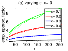
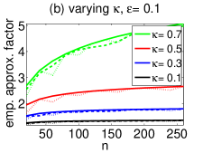
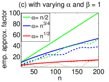
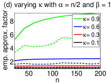
Figure 1: Minimization of $g_{\kappa}$ (Equation 41) for cardinality lower bound constraints. (a) fixed $\kappa=0$, $\alpha=n^{1/2+\epsilon},\beta=n^{2\epsilon}$ for varying $\epsilon$; (b) fixed $\epsilon=0.1$, but varying $\kappa$; (c) different choices of $\alpha$ for $\beta=1$; (d) varying $\kappa$ with $\alpha=n/2,\beta=1$. Dashed lines: MUB, dotted lines: EA, solid lines: theoretical bound. The results of EA are not visible in some instances since it obtains a factor of $1$.

Minimum submodular edge cover:

The minimum submodular edge cover involves finding an edge cover (subset of edges covering all vertices), with minimum submodular cost. This problem has been investigated in [25], and they show that this problem is $O(n)$ hard. Algorithm MUB provides an approximation guarantee which is no worse than $\frac{2n}{2+(n-2)(1-\kappa_{f})}$. We can show a almost matching hardness lower bound for this problem.

Theorem 5.9.

Given a submodular function, with curvature coefficient $\kappa_{f}$ and any $\epsilon,\delta>0$, there cannot exist a polynomial-time approximation algorithm, which achieves an approximation better than $\frac{n^{1-3\epsilon}}{2+(n^{1-3\epsilon}-2)(1-\kappa_{f})+2\delta\kappa_{f}}$ for the minimum submodular edge cover problem.

Proof.

We can use the construction of [25] to show this. However a simple observation shows that a perfect matching is also an edge cover, and hence the hardness of edge cover has to be at least as much as the hardness of perfect matchings. ∎

5.1 Experiments

We end this section by empirically demonstrating the performance of MUB and EA and their precise dependence on curvature. We focus on cardinality lower bound constraints, $\mathcal{C}=\{X\subseteq V:|X|\geq\alpha\}$ and the “worst-case” class of functions that has been used throughout this paper to prove lower bounds,

$$f^{R}(X)=\min\{|X\cap\bar{R}|+\beta,|X|,\alpha\},$$ (40)

where $\bar{R}=V\backslash R$ and $R\subseteq V$ is random set such that $|R|=\alpha$. We adjust $\alpha=n^{1/2+\epsilon}$ and $\beta=n^{2\epsilon}$ by a parameter $\epsilon$. The smaller $\epsilon$ is, the harder the problem. The function (40) has curvature $\kappa_{f}=1$. To obtain a function with specific curvature $\kappa$, we define

$$f^{R}_{\kappa}(X)=\kappa f(X)+(1-\kappa)|X|.$$ (41)

In all our experiments, we take the average over $20$ random draws of $R$. We first set $\kappa=1$ and vary $\epsilon$. Figure 1(a) shows the empirical approximation factors obtained using EA and MUB, and the theoretical bound. The empirical factors follow the theoretical results very closely. Empirically, we also see that the problem becomes harder as $\epsilon$ decreases. Next we fix $\epsilon=0.1$ and vary the curvature $\kappa$ in $f^{R}_{\kappa}$. Figure 1(b) illustrates that the theoretical and empirical approximation factors improve significantly as $\kappa$ decreases. Hence, much better approximations than the previous theoretical lower bounds are possible if $\kappa$ is not too large. This observation can be very important in practice. Here, too, the empirical upper bounds follow the theoretical bounds very closely.

Figures 1(c) and (d) show results for larger $\alpha$ and $\beta=1$. In Figure 1(c), as $\alpha$ increases, the empirical factors improve. In particular, as predicted by the theoretical bounds, EA outperforms MUB for large $\alpha$ and, for $\alpha\geq n^{2/3}$, EA finds the optimal solution. In addition, Figures 1(b) and (d) illustrate the theoretical and empirical effect of curvature: as $n$ grows, the bounds saturate and approximate a constant $1/(1-\kappa)$ – they do not grow polynomially in $n$. Overall, we see that the empirical results quite closely follow our theoretical results, and that, as the theory suggests, curvature significantly affects the approximation factors.

6 Conclusion and Discussion

In this paper, we study the effect of curvature on the problems of approximating, learning and minimizing submodular functions under constraints. We prove tightened, curvature-dependent upper bounds with almost matching lower bounds. These results complement known results for submodular maximization [7, 55]. Moreover, in [28], we also consider the role of curvature in submodular optimization problems over a class of submodular constraints. Given that the functional form and effect of the submodularity ratio proposed in [9] is similar to that of curvature, an interesting extension is the question of whether there is a single unifying quantity for both of these terms. Another open question is whether a quantity similar to curvature can be defined for subadditive functions, thus refining the results in [2, 1] for learning subadditive functions. Finally it also seems that the techniques in this paper could be used to provide improved curvature-dependent regret bounds for constrained online submodular minimization [34].

Acknowledgments: Special thanks to Kai Wei for pointing out that Corollary 3.5 holds and for other discussions, to Bethany Herwaldt for reviewing an early draft of this manuscript, and to the anonymous reviewers. This material is based upon work supported by the National Science Foundation under Grant No. (IIS-1162606), a Google and a Microsoft award, and by the Intel Science and Technology Center for Pervasive Computing. Stefanie Jegelka’s work is supported by the Office of Naval Research under contract/grant number N00014-11-1-0688, and gifts from Amazon Web Services, Google, SAP, Blue Goji, Cisco, Clearstory Data, Cloudera, Ericsson, Facebook, General Electric, Hortonworks, Intel, Microsoft, NetApp, Oracle, Samsung, Splunk, VMware and Yahoo!.

References

- Badanidiyuru et al. [2012] A. Badanidiyuru, S. Dobzinski, H. Fu, R. Kleinberg, N. Nisan, and T. Roughgarden. Sketching valuation functions. In SODA, pages 1025–1035, 2012.
- Balcan et al. [2011] M. F. Balcan, F. Constantin, S. Iwata, and L. Wang. Learning valuation functions. COLT, 2011.
- Balcan and Harvey [2012] N. Balcan and N. Harvey. Submodular functions: Learnability, structure, and optimization. In Arxiv preprint, 2012.
- Buchbinder et al. [2012] N. Buchbinder, M. Feldman, J. Naor, and R. Schwartz. A tight (1/2) linear-time approximation to unconstrained submodular maximization. In FOCS, 2012.
- Calinescu et al. [2007] G. Calinescu, C. Chekuri, M. Pal, and J. Vondrák. Maximizing a monotone submodular function under a matroid constraint. IPCO, 2007.
- Chekuri et al. [2011] C. Chekuri, J. Vondrák, and R. Zenklusen. Submodular function maximization via the multilinear relaxation and contention resolution schemes. STOC, 2011.
- Conforti and Cornuejols [1984] M. Conforti and G. Cornuejols. Submodular set functions, matroids and the greedy algorithm: tight worst-case bounds and some generalizations of the Rado-Edmonds theorem. Discrete Applied Mathematics, 7(3):251–274, 1984.
- Cunningham [1983] W. H. Cunningham. Decomposition of submodular functions. Combinatorica, 3(1):53–68, 1983.
- Das and Kempe [2011] A. Das and D. Kempe. Submodular meets spectral: Greedy algorithms for subset selection, sparse approximation and dictionary selection. In ICML, 2011.
- Delong et al. [2012] A. Delong, O. Veksler, A. Osokin, and Y. Boykov. Minimizing sparse high-order energies by submodular vertex-cover. In NIPS, 2012.
- Devanur et al. [2013] N. R. Devanur, S. Dughmi, R. Schwartz, A. Sharma, and M. Singh. On the approximation of submodular functions. arXiv preprint arXiv:1304.4948, 2013.
- Feige et al. [2007] U. Feige, V. Mirrokni, and J. Vondrák. Maximizing non-monotone submodular functions. SIAM J. COMPUT., 40(4):1133–1155, 2007.
- Feldman et al. [2011] M. Feldman, J. Naor, and R. Schwartz. A unified continuous greedy algorithm for submodular maximization. In Foundations of Computer Science (FOCS), 2011 IEEE 52nd Annual Symposium on, pages 570–579. IEEE, 2011.
- Fleischer and Iwata [2003] L. Fleischer and S. Iwata. A push-relabel framework for submodular function minimization and applications to parametric optimization. Discrete Applied Mathematics, 131(2):311–322, 2003.
- Fujishige [2005] S. Fujishige. Submodular functions and optimization, volume 58. Elsevier Science, 2005.
- Goel et al. [2009] G. Goel, C. Karande, P. Tripathi, and L. Wang. Approximability of combinatorial problems with multi-agent submodular cost functions. In FOCS, 2009.
- Goel et al. [2010] G. Goel, P. Tripathi, and L. Wang. Combinatorial problems with discounted price functions in multi-agent systems. In FSTTCS, 2010.
- Goemans et al. [2009] M. Goemans, N. Harvey, S. Iwata, and V. Mirrokni. Approximating submodular functions everywhere. In SODA, pages 535–544, 2009.
- Grötschel et al. [1981] M. Grötschel, L. Lovász, and A. Schrijver. The ellipsoid method and its consequences in combinatorial optimization. Combinatorica, 1(2):169–197, 1981.
- Grotschel et al. [1984] M. Grotschel, L. Lovász, and A. Schrijver. Geometric methods in combinatorial optimization. In Silver Jubilee Conf. on Combinatorics, pages 167–183, 1984.
- Hassin et al. [2007] R. Hassin, J. Monnot, and D. Segev. Approximation algorithms and hardness results for labeled connectivity problems. J Combinatorial Optimization, 14(4):437–453, 2007.
- Iwata [2002] S. Iwata. A fully combinatorial algorithm for submodular function minimization. In Proceedings of the thirteenth annual ACM-SIAM symposium on Discrete algorithms, pages 915–919. Society for Industrial and Applied Mathematics, 2002.
- Iwata [2003] S. Iwata. A faster scaling algorithm for minimizing submodular functions. SIAM Journal on Computing, 32(4):833–840, 2003.
- Iwata [2008] S. Iwata. Submodular function minimization. Mathematical Programming, 112(1):45–64, 2008.
- Iwata and Nagano [2009] S. Iwata and K. Nagano. Submodular function minimization under covering constraints. In In FOCS, pages 671–680. IEEE, 2009.
- Iwata and Orlin [2009] S. Iwata and J. Orlin. A simple combinatorial algorithm for submodular function minimization. In Proceedings of the twentieth Annual ACM-SIAM Symposium on Discrete Algorithms, pages 1230–1237. Society for Industrial and Applied Mathematics, 2009.
- Iwata et al. [2001] S. Iwata, L. Fleischer, and S. Fujishige. A combinatorial strongly polynomial algorithm for minimizing submodular functions. Journal of the ACM (JACM), 48(4):761–777, 2001.
- Iyer and Bilmes [2013] R. Iyer and J. Bilmes. Submodular optimization with submodular cover and submodular knapsack constraints. In NIPS, 2013.
- Iyer and Bilmes [2012a] R. Iyer and J. Bilmes. The submodular Bregman and Lovász-Bregman divergences with applications. In NIPS, 2012a.
- Iyer and Bilmes [2012b] R. Iyer and J. Bilmes. Algorithms for approximate minimization of the difference between submodular functions, with applications. In UAI, 2012b.
- Iyer et al. [2012] R. Iyer, S. Jegelka, and J. Bilmes. Mirror descent like algorithms for submodular optimization. NIPS Workshop on Discrete Optimization in Machine Learning (DISCML), 2012.
- Iyer et al. [2013] R. Iyer, S. Jegelka, and J. Bilmes. Fast semidifferential based submodular function optimization. In ICML, 2013.
- Jegelka [2012] S. Jegelka. Combinatorial Problems with submodular coupling in machine learning and computer vision. PhD thesis, ETH Zurich, 2012.
- Jegelka and Bilmes [2011a] S. Jegelka and J. Bilmes. Online submodular minimization for combinatorial structures. ICML, 2011a.
- Jegelka and Bilmes [2011b] S. Jegelka and J. A. Bilmes. Approximation bounds for inference using cooperative cuts. In ICML, 2011b.
- Jegelka and Bilmes [2011c] S. Jegelka and J. A. Bilmes. Submodularity beyond submodular energies: coupling edges in graph cuts. In CVPR, 2011c.
- Kohli et al. [2013] P. Kohli, A. Osokin, and S. Jegelka. A principled deep random field for image segmentation. In CVPR, 2013.
- Krause and Guestrin [2005] A. Krause and C. Guestrin. Near-optimal nonmyopic value of information in graphical models. In Proceedings of Uncertainity in Artificial Intelligence. UAI, 2005.
- Krause et al. [2006] A. Krause, C. Guestrin, A. Gupta, and J. Kleinberg. Near-optimal sensor placements: Maximizing information while minimizing communication cost. In IPSN, 2006.
- Lawler and Martel [1982] E. Lawler and C. Martel. Computing maximal “polymatroidal” network flows. Mathematics of Operations Research, 7(3):334–347, 1982.
- Lee et al. [2009a] J. Lee, V. Mirrokni, V. Nagarajan, and M. Sviridenko. Non-monotone submodular maximization under matroid and knapsack constraints. In STOC, pages 323–332. ACM, 2009a.
- Lee et al. [2009b] J. Lee, M. Sviridenko, and J. Vondrák. Submodular maximization over multiple matroids via generalized exchange properties. In APPROX, 2009b.
- Lin and Bilmes [2011a] H. Lin and J. Bilmes. Optimal selection of limited vocabulary speech corpora. In Interspeech, 2011a.
- Lin and Bilmes [2011b] H. Lin and J. Bilmes. A class of submodular functions for document summarization. In The 49th Meeting of the Assoc. for Comp. Ling. Human Lang. Technologies (ACL/HLT-2011), Portland, OR, June 2011b.
- Lin and Bilmes [2012] H. Lin and J. Bilmes. Learning mixtures of submodular shells with application to document summarization. In UAI, 2012.
- Nemhauser et al. [1978] G. Nemhauser, L. Wolsey, and M. Fisher. An analysis of approximations for maximizing submodular set functions—i. Mathematical Programming, 14(1):265–294, 1978.
- Nikolova [2010] E. Nikolova. Approximation algorithms for offline risk-averse combinatorial optimization, 2010.
- Orlin [2009] J. Orlin. A faster strongly polynomial time algorithm for submodular function minimization. Mathematical Programming, 118(2):237–251, 2009.
- Soto and Goemans [2010] J. Soto and M. Goemans. Symmetric submodular function minimization under hereditary family constraints. arXiv:1007.2140, 2010.
- Stobbe and Krause [2012] P. Stobbe and A. Krause. Learning fourier sparse set functions. In International Conference on Artificial Intelligence and Statistics (AISTATS), 2012.
- Sviridenko [2004] M. Sviridenko. A note on maximizing a submodular set function subject to a knapsack constraint. Operations Research Letters, 32(1):41–43, 2004.
- Svitkina and Fleischer [2008] Z. Svitkina and L. Fleischer. Submodular approximation: Sampling-based algorithms and lower bounds. In FOCS, pages 697–706, 2008.
- Valiant [1984] L. G. Valiant. A theory of the learnable. Communications of the ACM, 27(11):1134–1142, 1984.
- Vicente et al. [2008] S. Vicente, V. Kolmogorov, and C. Rother. Graph cut based image segmentation with connectivity priors. In Proc. CVPR, 2008.
- Vondrák [2010] J. Vondrák. Submodularity and curvature: the optimal algorithm. RIMS Kokyuroku Bessatsu, 23, 2010.
- Wan et al. [2002] P.-J. Wan, G. Calinescu, X.-Y. Li, and O. Frieder. Minimum-energy broadcasting in static ad hoc wireless networks. Wireless Networks, 8:607–617, 2002.
- Zhang et al. [2011] P. Zhang, J.-Y. Cai, L.-Q. Tang, and W.-B. Zhao. Approximation and hardness results for label cut and related problems. Journal of Combinatorial Optimization, 21(2):192–208, 2011.