On the persistence properties of the cross-coupled Camassa-Holm system

Abstract

In this paper we examine the evolution of solutions, that initially have compact support, of a recently-derived system [7] of cross-coupled Camassa-Holm equations. The analytical methods which we employ provide a full picture for the persistence of compact support for the momenta. For solutions of the system itself, the answer is more convoluted, and we determine when the compactness of the support is lost, replaced instead by an exponential decay rate.

1 Introduction

This paper is concerned with the persistence of compact support in solutions to a recently derived cross-coupled Camassa-Holm (CCCH) equation [7], which is given by

$$m_{t}+2v_{x}m+vm_{x} =0$$ (1a)

$$n_{t}+2u_{x}n+un_{x} =0,,$$ (1b)

where $m=u-u_{xx}$ and $n=v-v_{xx}$. This system generalises the celebrated Camassa-Holm (CH) equation [1], since for $u=v$ the system (2) reduces to two copies of the CH equation

$$m_{t}+2u_{x}m+um_{x}=0.$$

The CH equation models a variety of phenomena, including the propagation of unidirectional shallow water waves over a flat bed [1, 8, 12, 17, 16]. The CH equation possesses a very rich structure, being an integrable infinite-dimensional Hamiltonian system with a bi-Hamiltonian structure and an infinity of conservation laws [1, 4, 15]. It also has a geometric interpretation as a re-expression of the geodesic flow on the diffeomorphism group of the circle [14]. One of the most interesting features of the CH equation, perhaps, is the rich variety of solutions it admits. Some solutions exist globally, whereas others exist only for a finite length of time, modelling wave breaking [6, 3].

The CCCH equation can be derived from a variational principle as a n Euler-Lagrange system of equations for the Lagrangian

$$l(u,v)=\int_{\mathbb{R}}\left(uv+u_{x}v_{x}\right)\text{ d}x.$$

Alternatively it can be formulated as a two-component system of Euler-Poincaré (EP) equations in one dimension on $\mathbb{R}$ as follows,

$${\partial_{t}}m=-\,{\rm ad}^{*}_{\delta h/\delta m}m=-\,(vm)_{x}-mv_{x}\quad\hbox{with}\quad v:=\frac{\delta h}{\delta m}=K*n,$$

$${\partial_{t}}n=-\,{\rm ad}^{*}_{\delta h/\delta n}n=-\,(un)_{x}-nu_{x}\quad\hbox{with}\quad u:=\frac{\delta h}{\delta n}=K*m,$$

with $K(x,y)=\frac{1}{2}e^{-|x-y|}$ being the Green function of the Helmholtz operator, and $h$ being the Hamiltonian

$$h(n,m)=\int_{\mathbb{R}}n\,K*m\text{ d}x=\!\!\int_{\mathbb{R}}m\,K*n\text{ d}x.$$

This Hamiltonian system has two-component singular momentum map [13]

$$m(x,t)=\sum_{a=1}^{M}m_{a}(t)\,\delta(x-q_{a}(t)),\qquad n(x,t)=\sum_{b=1}^{N}n_{b}(t)\,\delta(x-r_{b}(t)).$$

The $M=N=1$ case is very simple for analysis [7]. If the initial conditions are $m_{1}(0)>0$ and $n_{1}(0)>0$ then one observes the so-called waltzing motion. It could be noted that for half of the waltzing period (half cycle) the two types of peakons exchange momentum amplitudes - see Fig. 1. The explicit solutions as well as other examples with waltzing peakons and compactons are given in [7].

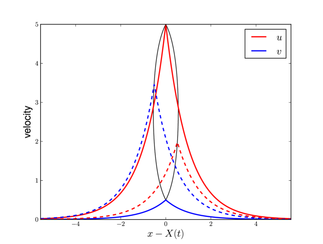
Figure 1: Plot showing velocity fields of a peakon-peakon pair with $m_{1}(0)=10$, $n_{1}(0)=1$ (solid lines). The dotted path indicates the subsequent path of the two peaks in the frame travelling at the particles mean velocity. For these initial conditions the total period for one orbit of the cycle is $T=3.6$. Also shown is the form of the two peakons at subsequent times $t=0.45+1.8n$, $n\in\mathbb{Z}$.

The aim of this study is to analyse the persistence of compact support for solutions of the system (2). In particular, we will examine whether the solution $m,n$, and in turn $u,v$, of (1a)-(1b), which initially have compact support, will continue to do so as they evolve. Solutions of the system which have compact support can be viewed as localized disturbances, and whether a “disturbance” which is initially localized propagates with a finite, or infinite speed, is a matter of great interest. We will see that some solutions will remain compactly supported at all future times of their existence, while others solution display an infinite speed of propagation and instantly lose their compact support. These results have analogues in the CH case, which is simply the CH equation [2, 9, 11].

2 Preliminaries

We may re-express equation (1) in terms of $u$ and $v$ as follows

$$u_{t}-u_{xxt}+2v_{x}u-2v_{x}u_{xx}+vu_{x}-vu_{xxx} =0,$$ (2a)

$$v_{t}-v_{xxt}+2u_{x}v-2u_{x}v_{xx}+uv_{x}-uv_{xxx} =0.$$ (2b)

From this form of the equations one observes that there are no terms with self-interaction (e.g. $uu_{x}$, $u_{x}u_{xx}$, $uu_{xxx}$ etc.) which justifies the name ’cross-coupled’.

If $p(x)=\frac{1}{2}e^{-|x|},\ x\in\mathbb{R}$, then $(1-\partial_{x}^{2})^{-1}f=p\ast f$ for all $f\in L^{2}(\mathbb{R})$ and so $p\ast m=u$, $p\ast n=v$, where $\ast$ denotes convolution in the spatial variable. Indeed,

$$u(x)=\frac{1}{2}e^{-x}\int_{-\infty}^{x}e^{y}m(y)\,dy+\frac{1}{2}e^{x}\int_{x}^{\infty}e^{-y}m(y)\,dy.$$ (3)

$$u_{x}(x)=-\frac{1}{2}e^{-x}\int_{-\infty}^{x}e^{y}m(y)\,dy+\frac{1}{2}e^{x}\int_{x}^{\infty}e^{-y}m(y)\,dy.$$ (4)

In other words, if we denote by $I_{1}(x)$ and $I_{2}(x)$ the integrals appearing in the first and the second term of (3), we have

$$u=I_{1}+I_{2},\qquad u_{x}=-I_{1}+I_{2}.$$ (5)

Applying the convolution operator to equation (2) we can re-express it in the form of a conservation law

$$(u+v)_{t}+\partial_{x}\left(uv+p\ast\left(2uv+u_{x}v_{x}\right)\right)=0,\quad x\in\mathbb{R},\ t\geq 0,$$ (6)

Thus $L=u+v$ is a density of the conserved momentum $\int(m+n)dx$. The representation (6) agrees with the CH reduction when $u=v$, cf. [9].

The Hamiltonian

$$H=\int(uv+u_{x}v_{x})dx$$

(in terms of $u$ and $v$) is of course another conserved quantity, the ’energy’ of the system, see more details in [7].

One can directly observe that (2) can be complexified in a natural way if the variables $u$, $v$ are assumed complex, while the independent variables $x$, $t$ are still real. Such a complexified system is remarkable with the fact that it admits the obvious reduction $u=\bar{v}$ which leads to a single scalar complex equation:

$$u_{t}-u_{xxt}+2\bar{u}_{x}u-2\bar{u}_{x}u_{xx}+\bar{u}u_{x}-\bar{u}u_{xxx}=0.$$ (7)

This is a geodesic equation for a complex $H^{1}$ metric, given by the Hamiltonian $H=\frac{1}{2}\int(|u|^{2}+|u_{x}|^{2})dx$.

Of course, if one reverts to real dependent variables according to $u=r+is$ then (7) leads to the coupled system

$$r_{t}-r_{xxt}+2(rr_{x}+ss_{x})-2(r_{x}r_{xx}+s_{x}s_{xx})-(rr_{xxx}+ss_{xxx}) =0,$$ (8a)

$$s_{t}-s_{xxt}+r_{x}s-rs_{x}-2(r_{x}s_{xx}-s_{x}r_{xx})-(rs_{xxx}-sr_{xxx}) =0.$$ (8b)

Unless it is explicitly specified that the variables $(u,v)$ are complex, we assume that they are real.

3 Results

In the following we let $T=T(u_{0},v_{0})>0$ denote the maximal existence time of the solutions $u(x,t),v(x,t)$ to the system (2) with the given initial data $u_{0}(x)$ and $v_{0}(x)$.

3.1 Persistence of compact support for the momenta

For the following, the flow prescribed by the system (1) is given by the two families of diffeomorphisms $\left\{\varphi(\cdot,t)\right\}_{t\in[0,T)}$, $\left\{\xi(\cdot,t)\right\}_{t\in[0,T)}$ as follows:

$$\left\{\begin{array}[]{l}\varphi_{t}(x,t)=v(\varphi(x,t),t),\\ \varphi(x,0)=x,\end{array}\right.\qquad\begin{array}[]{l}\xi_{t}(x,t)=u(\xi(x,t),t),\\ \xi(x,0)=x.\end{array}$$ (13)

Solving (13), we get

$$\varphi_{x}(x,t)=e^{\int_{0}^{t}v_{x}(\varphi(x,s),s)ds},\ \xi_{x}(x,t)=e^{\int_{0}^{t}u_{x}(\xi(x,s),s)ds}>0,$$ (14)

hence $\varphi(\cdot,t),\xi(\cdot,t)$ are increasing functions.

Lemma 3.1

Assume that $u_{0}$ and $v_{0}$ are such that $m_{0}=u_{0}-u_{0,xx}$ and $n_{0}=v_{0}-v_{0,xx}$ are nonnegative (nonpositive) for $x\in\mathbb{R}$. Then $m(x,t)$ and $n(x,t)$ remain nonnegative (nonpositive) for all $t\in[0,T)$.

• It follows from (1) that

  $$\frac{d\phantom{t}}{dt}m(\varphi(x,t),t)\varphi_{x}^{2}(x,t)=m_{t}\varphi_{x}^{2}+m_{x}\varphi_{t}\varphi_{x}^{2}+2m\varphi_{x}\varphi_{xt}$$

  $$=(m_{t}+2v_{x}m+vm_{x})\varphi_{x}^{2}=0,$$

  and

  $$\frac{d\phantom{t}}{dt}n(\xi(x,t),t)\xi_{x}^{2}(x,t)=n_{t}\xi_{x}^{2}+n_{x}\xi_{t}\xi_{x}^{2}+2m\xi_{x}\xi_{xt}$$

  $$=(n_{t}+2u_{x}n+un_{x})\xi_{x}^{2}=0.$$

  Therefore

  $$m(\varphi(x,t),t)\varphi_{x}^{2}(x,t)=m_{0}(x),\quad n(\xi(x,t),t)\xi_{x}^{2}(x,t)=n_{0}(x).$$ (15)

  Now, since $m_{0}(x),n_{0}(x)$ are nonnegative (nonpositive) then $m(x,t)$ and $n(x,t)$ remain nonnegative (nonpositive) for all $t\in[0,T)$.       

Lemma 3.2

Assume that $u_{0}$ is such that $m_{0}=u_{0}-u_{0,xx}$ has compact support, contained in the interval $[\alpha_{m_{0}},\beta_{m_{0}}]$ say, then for any $t\in[0,T)$, the function $x\mapsto m(x,t)$ has compact support contained in the interval $[\varphi(\alpha_{m_{0}},t),\varphi(\beta_{m_{0}},t)]$ for all $t\in[0,T)$. Similarly, if $n_{0}=v_{0}-v_{0,xx}$ has compact support, then the function $x\mapsto n(x,t)$ is compactly supported for all $t\in[0,T)$.

• From (15) and from the assumption that $m_{0}(x)$ is supported in the compact interval $[\alpha_{m_{0}},\beta_{m_{0}}]$, it follows directly that $m(\cdot,t)$ are compactly supported, with support contained in the interval $[\varphi(\alpha_{m_{0}},t),\varphi(\beta_{m_{0}},t)]$, for all $t\in[0,T)$. Similar reasoning applies to $n_{0}$.       

Relation (15) represents the conservation of momentum in the physical variables cf. discussion in [7].

3.2 On the evolution of $(u,v)$

In this subsection we are going to examine the general behaviour of the solution $(u,v)$ of (2) which is initially compactly supported. The following Theorem provides us with some information about the asymptotic behavior of the solution as it evolves over time - in general, the solution has an exponential decay as $|x|\rightarrow\infty$ for all future times $t\in[0,T)$.

Theorem 3.3

Let $(u,v)$ be a nontrivial solution of (2), with maximal time of existence $T>0$, and which is initially compactly supported on an interval $\mathcal{I}_{0}=[\alpha_{u_{0}},\beta_{u_{0}}]\times[\alpha_{v_{0}},\beta_{v_{0}}]$. Then we have

$$u(x,t)=\left\{\begin{array}[]{ll}\frac{1}{2}E^{u}_{+}(t)e^{-x}&\mbox{ for }x>\xi(\beta_{u_{0}},t),\\ \frac{1}{2}E^{u}_{-}(t)e^{x}&\mbox{ for }x<\xi(\alpha_{u_{0}},t),\end{array}\right.,$$ (18)

$$v(x,t)=\left\{\begin{array}[]{ll}\frac{1}{2}E^{v}_{+}(t)e^{-x}&\mbox{ for }x>\varphi(\beta_{v_{0}},t),\\ \frac{1}{2}E^{v}_{-}(t)e^{x}&\mbox{ for }x<\varphi(\alpha{v_{0}},t),\end{array}\right.$$ (21)

where $\alpha,\beta$ are defined in (22) below, and $E^{u}_{-},E^{u}_{+},E^{v}_{-},E^{v}_{+}$ are continuous functions, with $E^{u}_{+}(0)=E^{v}_{+}(0)=E^{u}_{-}(0)=E^{v}_{-}(0)=0$.

• Firstly, if $(u_{0},v_{0})$ is initially supported on the compact interval $\mathcal{I}_{0}=[\alpha_{u_{0}},\beta_{u_{0}}]\times[\alpha_{v_{0}},\beta_{v_{0}}]$ then so too is $m_{0}$, and from the proof Lemma 3.2 it follows that $\left(m(\cdot,t),n(\cdot,t)\right)$ is compactly supported, with its support contained in the interval $\mathcal{I}_{t}=[\xi(\alpha,t),\xi(\beta,t)]\times[\varphi(\alpha,t),\varphi(\beta,t)]$ for fixed $t\in[0,T)$. Here

  $$\alpha=\min\{\alpha_{u_{0}},\alpha_{v_{0}}\},\ \beta=\max\{\beta_{u_{0}},\beta_{v_{0}}\}.$$ (22)

  We use the relation $u=p\ast m$ to write

  $$u(x)=\frac{1}{2}e^{-x}\int_{-\infty}^{x}e^{y}m(y)\,dy+\frac{1}{2}e^{x}\int_{x}^{\infty}e^{-y}m(y)\,dy,$$

  and then we define our functions

  $$E^{u}_{+}(t)=\int_{\xi(\alpha,t)}^{\xi(\beta,t)}e^{y}m(y,t)\,dy\quad\mbox{ and }E^{u}_{-}(t)=\int_{\xi(\alpha,t)}^{\xi(\beta,t)}e^{-y}m(y,t)dy.$$ (23)

  We have

  $$\begin{array}[]{ll}u(x,t)=\frac{1}{2}e^{-x}E^{u}_{+}(t),&x>\xi(\beta,t),\\ u(x,t)=\frac{1}{2}e^{x}E^{u}_{-}(t),&x<\xi(\alpha,t),\end{array}$$ (24)

  and therefore from differentiating (24) directly we get

  $$\begin{array}[]{ll}\frac{1}{2}e^{-x}E^{u}_{+}(t)=u(x,t)=-u_{x}(x,t)=u_{xx}(x,t),&x>\xi(\beta,t),\\ \frac{1}{2}e^{x}E^{u}_{-}(t)=u(x,t)=u_{x}(x,t)=u_{xx}(x,t),&x<\xi(\alpha,t).\end{array}$$

  Since $u(\cdot,0)$ is supported in the interval $[\alpha,\beta]$, we have $E^{u}_{+}(0)=E^{u}_{-}(0)=0$, as we can see by taking integration by parts where the boundary terms vanish.       

Corollary 3.4

If in addition $m_{0}(x)$ and $n_{0}(x)$ are everywhere nonnegative (nonpositive), then the solution $(u,v)$ (if nontrivial) loses its compactness immediately.

• Indeed, in order for an nontrivial solution to stay compact one needs $E^{u}_{\pm}(t)\equiv 0$, $E^{v}_{\pm}(t)\equiv 0$ for all $t\in[0,T]$. However from Lemma 3.1 it follows that $m(x,t)$ and $n(x,t)$ remain everywhere nonnegative (nonpositive) and thus the quantities $E^{u}_{\pm}(t)$, $E^{v}_{\pm}(t)$ defined e.g. in (23) are positive (negative) for all $t\in(0,T]$ in the case of a nontrivial solution.       

From (6) we know that $L=u+v$ is a density of a conserved quantity and as such it deserves a special attention. From Theorem 3.3 one can find the asymptotics of $L$ as $x\to\pm\infty$ as

$$L\to\frac{1}{2}E_{\pm}(t)e^{-|x|}$$

where $E_{\pm}\equiv E^{u}_{\pm}+E^{v}_{\pm}$. Since the nature of the solution that we expect is several coupled ’waltzing’ waves, i.e. the maximum elevations of $u(x,t)$ and $v(x,t)$ increase and decrease with time in the waltzing process. In other words the functions $E^{u}_{\pm}(t)$ and $E^{v}_{\pm}(t)$ are in general non-monotonic functions of $t$. However in some cases a monotonic property holds for the conserved density $L$:

Theorem 3.5

If $(u,v)$ is an initially compactly supported solution and in addition $m_{0}(x)$ and $n_{0}(x)$ are everywhere nonnegative (nonpositive), then the quantity $E_{+}(t)$ is a monotonically increasing function and $E_{-}(t)$ is a monotonically decreasing function.

• Indeed, from Lemma 3.1 it follows that $m(x,t)$ and $n(x,t)$ remain everywhere nonnegative (nonpositive) and from the explicit form of the inverse Helmholtz operator $u(x,t)$ and $v(x,t)$ remain everywhere nonnegative (nonpositive). Since $m(\cdot,t)$ is supported in the interval $[\xi(\alpha,t),\xi(\beta,t)]$, for each fixed $t$, the derivative is given by

  $$\frac{\mathrm{d}E^{u}_{+}(t)}{\mathrm{d}t}=\int_{\xi(\alpha,t)}^{\xi(\beta,t)}e^{y}m_{t}(y,t)\mathrm{d}y=\int_{-\infty}^{\infty}e^{y}m_{t}(y,t)\mathrm{d}y.$$

  Similarly, if we define

  $$E^{v}_{+}(t)=\int_{\varphi(\alpha,t)}^{\varphi(\beta,t)}e^{y}m(y,t)\,dy\quad\mbox{ and }E^{v}_{-}(t)=\int_{\varphi(\alpha,t)}^{\varphi(\beta,t)}e^{-y}m(y,t)dy,$$

  then $E^{v}_{+}(0)=E^{v}_{-}(0)=0$, and

  $$\frac{\mathrm{d}E^{v}_{+}(t)}{\mathrm{d}t}=\int_{-\infty}^{\infty}e^{y}n_{t}(y,t)\mathrm{d}y.$$

  From 1b and integration by parts we have

  $$\frac{\mathrm{d}E_{+}(t)}{\mathrm{d}t}=\int_{-\infty}^{\infty}e^{y}(m_{t}(y,t)+n_{t}(y,t))\,dx$$

  $$=-\int_{\mathbb{R}}e^{x}\left(2v_{x}(u-u_{xx})+v(u-u_{xx})_{x}+2u_{x}(v-v_{xx})+u(v-v_{xx})_{x}\right)\,dx$$

  $$=\int_{-\infty}^{\infty}e^{y}\left(2uv+u_{x}v_{x}\right)\,dy,\ \quad t\in[0,T),$$

  where all boundary terms after integration by parts vanish, since the functions $m(\cdot,t)$, $n(\cdot,t)$ have compact support and $u(\cdot,t)$, $v(\cdot,t)$ decay exponentially at $\pm\infty$, for all $t\in[0,T)$. Using (5) for $u=I_{1}^{u}+I_{2}^{u}$, $u_{x}=-I_{1}^{u}+I_{2}^{u}$, $v=I_{1}^{v}+I_{2}^{v}$, $v_{x}=-I_{1}^{v}+I_{2}^{v}$, and noticing that all integrals $I_{1,2}^{u,v}$ are all nonnegative (nonpositive), we have that

  $$2uv+u_{x}v_{x}=3I_{1}^{u}I_{1}^{v}+I_{2}^{u}I_{1}^{v}+I_{1}^{u}I_{2}^{v}+3I_{2}^{u}I_{2}^{v}$$

  and thus

  $$\frac{\mathrm{d}E_{+}(t)}{\mathrm{d}t}>0.$$ (26)

  Similarly, we have

  $$\frac{\mathrm{d}E_{-}(t)}{\mathrm{d}t}=\int_{-\infty}^{\infty}e^{-y}(m_{t}(y,t)+n_{t}(y,t))\,dx$$

  $$=-\int_{-\infty}^{\infty}e^{-y}\left(2uv+u_{x}v_{x}\right)\,dy<0,\ \ t\in[0,T)$$ (27)

  for analogous reasons as before.       

3.3 Evolution in the case $u=\bar{v}$ when initially compactly supported

Some analytical results can be established in the case $u=\bar{v}$, for example one can prove immediately the analogue of Theorem 3.5:

Theorem 3.6

If $u=\bar{v}$ is initially compactly supported, then $E_{-}=(E^{u}_{-}+E^{v}_{-})(t)$ is a decreasing function, with $E_{-}(0)=0$, and $E_{+}(t)$ is increasing, with $E_{+}(0)=0$.

• Follows the lines of the proof of Theorem 3.5. In this case $2uv+u_{x}v_{x}=2|u|^{2}+|u_{x}|^{2}\geq 0$ and for nontrivial solutions this expresion is at least somewhere positive.       

The following Lemma is proved by making extensive use of relation (3).

Lemma 3.7

[9] Let $(u,v)$ be a solution of system (2), and suppose $u$ is such that $m=u-u_{xx}$ has compact support. Then, for each fixed time $0<t<T$, $u$ has compact support if and only if

$$\int_{\mathbb{R}}e^{x}m(x)\,dx=\int_{\mathbb{R}}e^{-x}m(x)\,dx=0.$$ (28)

The equivalent relation holds for the functions $v$ and $n$.

We now establish a relation which is satisfied by solutions of (2) whose support remains compact throughout their evolution. This relation will have profound implications for solutions $(u,v)$ of (2) which have a direct relation to each other, as we see in Corollary (3.9).

Theorem 3.8

Let us assume that the functions $u_{0},v_{0}$ have compact support, and let $T>0$ be the maximal existence time of the solutions $u(x,t),v(x,t)$ which are generated by this initial data. If, for every $t\in[0,T)$, the function $x\mapsto\left(u(x,t),v(x,t)\right)$ has compact support, then

$$\int_{\mathbb{R}}e^{x}\left(2uv+u_{x}v_{x}\right)\,dx=\int_{\mathbb{R}}e^{-x}\left(2uv+u_{x}v_{x}\right)\,dx=0\ \ \mbox{ for }t\in[0,T).$$ (29)

• By the assumptions of this theorem, Lemma 3.7 applies. Using (2) and differentiating the left hand side of (28) with respect to $t$ we get

  $$\frac{d}{dt}\int_{\mathbb{R}}e^{x}\left(m+n\right)\,dx=-\int_{\mathbb{R}}e^{x}\left(2v_{x}m+vm_{x}+2u_{x}n+un_{x}\right)\,dx$$

  $$=\int_{\mathbb{R}}e^{x}\left(2uv+u_{x}v_{x}\right)\,dx=0,$$

  similarly to the proof of Theorem 3.5. The final equality follows from the fact that identity (28) holds for all $t\in[0,T)$, by Lemma 3.7.

  Similarly, we get

  $$\frac{d}{dt}\int_{\mathbb{R}}e^{-x}\left(m+n\right)\,dx=-\int_{\mathbb{R}}e^{-x}\left(2uv+u_{x}v_{x}\right)\,dx=0.$$ (30)

  Therefore,

  $$\int_{\mathbb{R}}e^{x}\left(2uv+u_{x}v_{x}\right)\,dx=\int_{\mathbb{R}}e^{-x}\left(2uv+u_{x}v_{x}\right)\,dx=0\quad t\in[0,T).$$ (31)

  The expression under the integral on the right hand side of this relation must be identically zero by (28). This completes the proof.       

Corollary 3.9

Let us suppose that $u(x,t)=\bar{v}(x,t)$. Then the only solution $(u,v)$ of (2) which is compactly supported over a positive time interval is the trivial solution $u\equiv v\equiv 0$. That is to say, any non-trivial solution $(u,v)$ of (2) which is initially compactly supported instantaneously loses this property, and so has an infinite propagation speed.

• The statement follows directly from relations in (31).       

3.4 Global solutions for nonnegative $m_{0},n_{0}$

From (3) and (4) it follows that

$$u(x,t)+u_{x}(x,t)=e^{x}\int_{x}^{\infty}e^{-y}m(y,t)\,dy.$$ (32)

Thus the nonnegativity of $m(x,t)$, $n(x,t)$, ensures $u_{x}(x,t)\geq-u(x,t)$ and similarly $v_{x}(x,t)\geq-v(x,t)$, preventing blowup in finite time, because the solution $(u,v)$ is uniformly bounded as long as it exists.

Blowup however might be possible if $m(x,0)$, $n(x,0)$ take both positive and negative values.

4 Conclusions

In the presented study we analysed the behavior of the solutions of the CCCH system when $m,n$ are initially compactly supported and (i) initially $u,v$ everywhere nonpositive/nonnegative (ii) $u=\bar{v}$. In both cases the result is that the compactness property is lost immediately, i.e. for any time $t>0$. Asymptotically the solutions decay exponentially to zero, such that $u+v$ decays to zero monotonically. The exponential decay is already observed in the case of the peakon solutions, where $m,n$ are supported only at finite number of points.

5 Acknowledgments

We are grateful to our friend and colleague James Percival for providing us the figure. The work of RII is supported by the Science Foundation Ireland (SFI), under Grant No. 09/RFP/MTH2144. The work by DDH was partially supported by Advanced Grant 267382 FCCA from the European Research Council.

References

• [1] R. Camassa and D. Holm, An integrable shallow water equation with peaked solitons, Phys. Rev. Lett. 71 (1993), 1661–1664.
• [2] A. Constantin, Finite Propagation Speed for the Camassa-Holm Equation, J. Math. Phys. 46 (2005), (023506).
• [3] A. Constantin and J. Escher, Wave breaking for nonlinear nonlocal shallow water equations, Acta Mathematica 181 (1998), 229–243.
• [4] A. Constantin, V. S. Gerdjikov and R. Ivanov, Generalized Fourier transform for the Camassa-Holm hierarchy, Inverse Problems 23 (2007), 1565–1597.
• [5] A. Constantin and R. Ivanov, On an integrable two-component Camassa-Holm shallow water system, Phys. Lett. A 372 (2008), 7129–7132.
• [6] A. Constantin and H. P. McKean, A shallow water equation on the circle, Comm. Pure Appl. Math. 52 (1999), 949–982.
• [7] C. Cotter, D. D. Holm, R. I. Ivanov and J. R. Percival Waltzing peakons and compacton pairs in a cross-coupled Camassa-Holm equation, J. Physics A 44 (2011), 265205 (28pp).
• [8] H. R. Dullin, G. A. Gottwald and D. D. Holm, On asymptotically equivalent shallow water wave equation, Phys. D 190 (2004), 1–14.
• [9] D. Henry, Compactly supported solutions of the Camassa-Holm equation, J. Nonlinear Math. Phys. 12 (2005), 342–347.
• [10] D. Henry, Persistence properties for a family of nonlinear partial differential equations, Nonlinear Anal. 70 (2009), 1565–1573.
• [11] D. Henry, Compactly supported solutions of a family of nonlinear partial differential equations, Dyn. Contin. Discrete Impuls. Syst. Ser. A 15 (2008), 145–150.
• [12] D. Holm and R. Ivanov, Smooth and peaked solitons of the Camassa-Holm equation and applications, J. of Geometry and Symmetry in Physics, 22 (2011) 13-49.
• [13] Holm, D. D. and Marsden, J. E. [2004] Momentum Maps and Measure-valued Solutions (Peakons, Filaments and Sheets) for the EPDiff Equation. In: The Breadth of Symplectic and Poisson Geometry, Progr. Math. 232, edited by J. E. Marsden and T. S. Ratiu (Boston: BirkhΓ€user) pp 203–235.
• [14] Holm, D. D., Marsden, J. E. and Ratiu, T. S. [1998] The Euler–PoincarΓ© equations and semidirect products with applications to continuum theories, Adv. in Math. 137, 1–81; Ibid [1998] Euler–PoincarΓ© models of ideal fluids with nonlinear dispersion Phys. Rev. Lett. 349, 4173–4177.
• [15] R. Ivanov, Extended Camassa-Holm hierarchy and conserved quantities, Z. Naturforsch. A 61 (2006), 133–138.
• [16] R. Ivanov, Water waves and integrability, Philos. Trans. R. Soc. Lond. Ser. A 365 (2007), 2267–2280.
• [17] R. S. Johnson, Camassa-Holm, Korteweg-de Vries and related models for water waves, J. Fluid Mech. 455 (2002), 63–82.