Crossover from Electromagnetically Induced Transparency to Autler-Townes Splitting in Open Ladder Systems with Doppler Broadening

Abstract

We propose a general theoretical scheme to investigate the crossover from electromagnetically induced transparency (EIT) to Autler-Townes splitting (ATS) in open ladder-type atomic and molecular systems with Doppler broadening. We show that when the wavenumber ratio $k_{c}/k_{p}\approx-1$, EIT, ATS, and EIT-ATS crossover exist for both ladder-I and ladder-II systems, where $k_{c}$ ($k_{p}$) is the wavenumber of control (probe) field. Furthermore, when $k_{c}/k_{p}$ is far from $-1$ EIT can occur but ATS is destroyed if the upper state of the ladder-I system is a Rydberg state. In addition, ATS exists but EIT is not possible if the control field used to couple the two lower states of the ladder-II system is a microwave field. The theoretical scheme developed here can be applied to atoms, molecules, and other systems (including Na₂ molecules, and Rydberg atoms), and the results obtained may have practical applications in optical information processing and transformation.

I INTRODUCTION

In recent years, much attention has been paid to the study of electromagnetically induced transparency (EIT), a quantum interference effect induced by a strong control field, by which the optical absorption of a probe field in resonant three-level atomic systems can be largely suppressed. In addition to the interest in fundamental research, EIT has many important applications in slow light and quantum storage, nonlinear optics at low-light level, precision laser spectroscopy, and so on Fleischhauer2005 .

The most prominent character of EIT is the opening of a transparency window in probe-field absorption spectra. However, the occurrence of transparency window is not necessarily due to EIT effect. In 1955, Autler and Townes at showed that the absorption spectrum of molecular transition can split into two Lorentzian lines (doublet) when one of two levels involved in the transition is coupled to a third one by a strong microwave field. Such doublet is now called Autler-Townes splitting (ATS) and has also been intensively investigated in atomic and molecular spectroscopy coh .

Although both EIT and ATS effects can open transparency windows in probe absorption spectra, the physical mechanisms behind them are quite different. EIT is resulted from a quantum destructive interference between two competing transition pathways, whereas ATS is a dynamic Stark shift caused by a gap between two resonances. Usually, it is not easy to distinguish EIT and ATS by simply looking at the appearance of absorption spectra.

Because EIT and ATS are two typical phenomena appeared widely in laser spectroscopy and have many applications, it is necessary to develop an effective technique to distinguish the difference between them. In 1997, Agarwal Agarwal1997 proposed a spectrum decomposition method, by which the probe-field absorption spectra of cold three-level atomic systems were decomposed into two absorptive contributions plus two interference contributions. Recently, this method was used to clarify EIT and ATS in a more general way Anisimov2008 ; Tony2010 ; Anisimov2011 . In a recent work, an experimental investigation on EIT-ATS crossover was carried out giner . Very recently, the spectrum decomposition method was adopted to investigate the EIT-ATS crossover in $\Lambda$- and $V$-type molecular systems with Doppler broadening tan2013 ; Zhu2013 .

In the study of EIT and ATS, several typical three-level systems (i.e. $\Lambda$, $V$, and ladder) note00 are widely used. For ladder systems, there are two typical configurations, with the level diagrams and excitation schemes shown in Figs. 1(a) and 1(b) below, called here as ladder-I (or upper-level-driven ladder system; Fig. 1(a) ) and ladder-II (or lower-level-driven ladder system; Fig. 1(b) ), respectively. The so-called upper-level-driven (lower-level-driven) means that the control field couples the two upper (lower) levels of the system. In recent years, much interest has been focused on the Rydberg excitations in cold and hot atomic gases, where ladder-type excitation schemes are widely employed saf ; pri1 ; sevi ; moh1 ; moh2 ; wea ; rai ; pri .

In this article, we propose a general theoretical scheme to investigate the crossover from electromagnetically induced transparency (EIT) to Autler-Townes splitting (ATS) in open ladder-type atomic and molecular systems with Doppler broadening. We show that when the wavenumber ratio $k_{c}/k_{p}\approx-1$, EIT, ATS, and EIT-ATS crossover exist for both ladder-I and ladder-II systems, where $k_{c}$ ($k_{p}$) is the wavenumber of control (probe) field. Furthermore, when $k_{c}/k_{p}$ is far from $-1$ EIT can occur but ATS is destroyed if the upper state of the ladder-I system is a Rydberg state. In addition, ATS exists but EIT is not possible if the control field used to couple the two lower states of the ladder-II system is a microwave field. The theoretical scheme developed and the results obtained here can be applied to various ladder systems (including hot gases of Rubidium atoms, Na₂ molecules, and Rydberg atoms).

Before proceeding, we note that many studies exist on the study of ladder systems. Except for EIT and ATS Agarwal1997 ; Tony2010 ; saf ; moh1 ; moh2 ; wea ; rai ; pri ; pri1 ; sevi ; Lazoudis2008 ; Yang1997 ; Yong1995 ; Julio1995 ; Lee2000 ; Jason2001 ; Qi2002 ; Ahmed2006 ; Ahmed2007 ; Ray2007 ; Moon ; Kubler2010 ; gor ; petro ; ate , other related investigations have also been carried out, including Rabi oscillations dudin ; Huber2011 , coherent population transfer schemp , quantum nonlinear optics at single-photon level Peyr , fast entanglement generation Bari , and microwave electrometry with Rydberg atoms Sedl . However, to the best of our knowledge no systematic analysis on the crossover from EIT to ATS in ladder systems has been carried out up to now; furthermore, no theory on the EIT-ATS crossover in open ladder systems with Doppler broadening has been presented. Our theoretical scheme is valid for both atoms, molecules, and other systems, and can elucidate various quantum interference characters (EIT, ATS, and EIT-ATS crossover) in a clear way. The results obtained here are not only useful for understanding the detailed feature of quantum interference in multi-level systems and guiding new experimental findings, but also may have promising applications in atomic and molecular spectroscopy, light and quantum information processing, etc.

The article is arranged as follows. In the next section, we describe the theoretical model. In Sec. III and Sec. IV, the quantum interference characters of the ladder-I and ladder-II systems are analyzed, respectively. Finally, in the last section we summarize the main results obtained in this work.

II MODEL

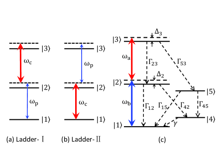
Figure 1: (Color online) (a) Ladder-I system, where states $|3\rangle$ and $|2\rangle$ are coupled by the control field with center angular frequency $\omega_{c}$, and states $|2\rangle$ and $|1\rangle$ are coupled by the probe field with center angular frequency $\omega_{p}$; (b) Ladder-II system. (c) Open ladder system. The state $|2\rangle$ couples to the state $|3\rangle$ by field $a$ (with center angular frequency $\omega_{a}$) and the ground state $|1\rangle$ by field $b$ (with center angular frequency $\omega_{b}$). $\Delta_{2}$ and $\Delta_{3}$ are detunings, $\Gamma_{jl}$ are population decay rates from $|l\rangle$ to $|j\rangle$, and $\gamma$ is the transit rate. Particles occupying the state $|2\rangle$ ($|3\rangle$) may decay to other states besides $|1\rangle$ ($|2\rangle$). Levels $|4\rangle$ and $|5\rangle$ denote these other states rendering the system open.

We consider a hot gas consisting of atoms or molecules, where particles have three resonant levels (i.e. ground state $|1\rangle$, intermediate state $|2\rangle$, and upper state $|3\rangle$) with a ladder configuration (Fig. 1(c) ) Ahmed2007 . Especially, the upper state $|3\rangle$ may be a Rydberg state. Two laser fields with central angular frequency $\omega_{a}$ and $\omega_{b}$ couple to the transition $|2\rangle\leftrightarrow|3\rangle$ and $|1\rangle\leftrightarrow|2\rangle$, respectively. The electric field vector is $\mathbf{E}=\sum_{l=a,b}\mathbf{e}_{l}{\cal E}_{l}{\rm exp}[i({\bf k}_{l}\cdot{\bf r}-\omega_{l}t)]+$c.c., where $\mathbf{e}_{l}$ $(k_{l})$ is the unit polarization vector (wavenumber) of the electric field component with the envelope ${\cal E}_{l}$ $(l=a,b)$.

We assume the system is open, i.e. particles occupying the state $|2\rangle$ ($|3\rangle$) can follow various relaxation pathways and decay into other states besides $|1\rangle$ ($|2\rangle$). For simplicity, all these other states are represented by states $|4\rangle$ and $|5\rangle$ Ahmed2007 . In the figure, $\Delta_{2}$ and $\Delta_{3}$ are detunings, $\Gamma_{jl}$ is the population decay rate from state $|l\rangle$ to state $|j\rangle$, $\gamma$ is the beam-transit rate added to account for the rate with which particles escape the interaction region (significant only for the level $|4\rangle$ since it cannot radiatively decay).

Under electric-dipole and rotating-wave approximations, the interaction Hamiltonian of the system in interaction picture reads

$${\cal H}_{\rm int}=-\hbar(\Omega_{a}e^{i[\mathbf{k}_{a}\cdot(\mathbf{r}+\mathbf{v}t)-\omega_{a}t]}|3\rangle\langle 2|+\Omega_{b}e^{i[\mathbf{k}_{b}\cdot(\mathbf{r}+\mathbf{v}t)-\omega_{b}t]}|2\rangle\langle 1|+{\rm h.c.}),$$ (1)

where $\Omega_{a}=\bm{\mu}_{32}\cdot{\cal E}_{a}/\hbar$ ($\Omega_{b}=\bm{\mu}_{21}\cdot{\cal E}_{b}/\hbar$) is the half Rabi-frequency of the field $a$ (field $b$), with $\bm{\mu}_{jl}$ being the electric-dipole matrix element associated with the transition from the state $|l\rangle$ to the state $|j\rangle$. The optical Bloch equation in the interaction picture is

$$i\frac{\partial}{\partial t}\sigma_{11}-i\Gamma_{12}\sigma_{22}-i\gamma\sigma_{44}-i\Gamma_{15}\sigma_{55}+\Omega_{b}^{*}\sigma_{21}-\Omega_{b}\sigma_{21}^{*}=0,$$ (2a)

$$i\frac{\partial}{\partial t}\sigma_{22}+i\Gamma_{2}\sigma_{22}-i\Gamma_{23}\sigma_{33}+\Omega_{b}\sigma_{21}^{*}+\Omega_{a}^{*}\sigma_{32}-\Omega_{b}^{*}\sigma_{21}-\Omega_{a}\sigma_{32}^{*}=0,$$ (2b)

$$i\frac{\partial}{\partial t}\sigma_{33}+i\Gamma_{3}\sigma_{33}+\Omega_{a}\sigma_{32}^{*}-\Omega_{a}^{*}\sigma_{32}=0,$$ (2c)

$$i\frac{\partial}{\partial t}\sigma_{44}+i\gamma\sigma_{44}-i\Gamma_{42}\sigma_{22}-i\Gamma_{45}\sigma_{55}=0,$$ (2d)

$$i\frac{\partial}{\partial t}\sigma_{55}+i\Gamma_{5}\sigma_{55}-i\Gamma_{53}\sigma_{33}=0,$$ (2e)

$$(i\frac{\partial}{\partial t}+d_{21})\sigma_{21}+\Omega_{a}^{*}\sigma_{31}+\Omega_{b}(\sigma_{11}-\sigma_{22})=0,$$ (2f)

$$(i\frac{\partial}{\partial t}+d_{31})\sigma_{31}-\Omega_{b}\sigma_{32}+\Omega_{a}\sigma_{21}=0,$$ (2g)

$$(i\frac{\partial}{\partial t}+d_{32})\sigma_{32}-\Omega_{b}^{*}\sigma_{31}+\Omega_{a}(\sigma_{22}-\sigma_{33})=0,$$ (2h)

where $d_{21}=-\mathbf{k}_{b}\cdot\mathbf{v}+\Delta_{2}+i\gamma_{21}$, $d_{31}=-(\mathbf{k}_{b}+\mathbf{k}_{a})\cdot\mathbf{v}+\Delta_{3}+i\gamma_{31}$, $d_{32}=-\mathbf{k}_{a}\cdot\mathbf{v}+\Delta_{3}-\Delta_{2}+i\gamma_{32}$ with $\gamma_{jl}=(\Gamma_{j}+\Gamma_{l})/2+\gamma_{jl}^{{\rm col}}\ (j,l=1,2,3)$. Here, $\bf{v}$ is the thermal velocity of the particles, $\Gamma_{j}$ denotes the total population decay rates out of levels $|j\rangle$, defined by $\Gamma_{j}=\sum_{l\neq j}\Gamma_{lj}$. The quantity $\gamma_{jl}^{{\rm col}}$ is the dephasing rate due to processes that are not associated with population transfer, such as elastic collisions.

The evolution of the electric field is governed by the Maxwell equation

$$\nabla^{2}{\bf E}-\frac{1}{c^{2}}\frac{\partial^{2}{\bf E}}{\partial t^{2}}=\frac{1}{\epsilon_{0}c^{2}}\frac{\partial^{2}{\bf P}}{\partial t^{2}}.$$ (3)

Due to the Doppler effect, the electric polarization intensity of the system reads

$${\bf P}={\cal N}\int_{-\infty}^{\infty}dvf(v)\left[\bm{\mu}_{12}\sigma_{21}e^{i(k_{b}z-\omega_{b}t)}+\bm{\mu}_{23}\sigma_{32}e^{i(k_{a}z-\omega_{a}t)}+{\rm c.c.}\right],$$ (4)

where ${\cal N}$ is particle concentration and $f(v)=e^{-(v/v_{T})^{2}}/(\sqrt{\pi}v_{T})$ is Maxwellian velocity distribution function, where $v_{T}=(2k_{B}T/M)^{1/2}$ is the most probable speed at temperature $T$ with $k_{B}$ the Boltzmann constant and $M$ the particle mass. For simplicity and without loss of generality, we have assumed the two laser fields propagate along the $z$ direction with a counter-propagating configuration, i.e. ${\bf k}_{a,b}=(0,0,k_{a,b})$ with $k_{b}=-k_{a}$ in order to suppress the first-order Doppler effect.

Note that the model given above is valid also for a closed ladder system, which can be obtained by simply taking $\Gamma_{15}=\Gamma_{42}=\Gamma_{45}=\Gamma_{53}=\gamma=0$; furthermore, if the system is not only closed but also cold, one has $\Gamma_{15}=\Gamma_{42}=\Gamma_{45}=\Gamma_{53}=\gamma=0$ and $f(v)=\delta(v)$.

III Quantum interference character of ladder-I system

III.1 Linear dispersion relation

When the laser field $a$ (field $b$) is taken as the control (probe) field, the system is the ladder-I system (i.e. $\omega_{a}=\omega_{c}$, $\omega_{b}=\omega_{p}$; see Fig. 1(a) ). In this case, under slowly varying envelope approximation (SVEA) the Maxwell Eq. (3) is reduced to the form

$$i\left(\frac{\partial}{\partial z}+\frac{1}{c}\frac{\partial}{\partial t}\right)\Omega_{b}+\kappa_{12}\int_{-\infty}^{\infty}dvf(v)\sigma_{21}(v)=0,$$ (5)

where $\kappa_{12}={\cal N}\omega_{b}|\bm{\mu}_{21}|^{2}/(2\hbar\varepsilon_{0}c)$ with $c$ is the light speed in vacuum.

The base state (zero-order) solution of the system, i.e. the steady-state solution of the MB Eqs. (2) and (5) for $\Omega_{b}=0$ is given by $\sigma_{11}^{(0)}=1$, $\sigma_{jl}^{(0)}=0$ ($j,l\neq 1$). When the probe field is switched on, the system will involve into time-dependent state. At the first order of $\Omega_{b}$, the population and the coherence between the states $|2\rangle$ and $|3\rangle$ are not changed, but

$$\Omega_{b}^{(1)}=Fe^{i\theta}$$ (6a)

$$\sigma_{21}^{(1)}=\frac{\omega+d_{31}}{|\Omega_{a}|^{2}-(\omega+d_{21})(\omega+d_{31})}Fe^{i\theta},$$ (6b)

$$\sigma_{31}^{(1)}=-\frac{\Omega_{a}}{|\Omega_{a}|^{2}-(\omega+d_{21})(\omega+d_{31})}Fe^{i\theta},$$ (6c)

here $F$ is a constant and $\theta=K(\omega)z-\omega t$. The linear dispersion relation $K(\omega)$ reads

$$K(\omega)=\frac{\omega}{c}+\kappa_{12}\int_{-\infty}^{\infty}dvf(v)\frac{\omega+d_{31}}{|\Omega_{a}|^{2}-(\omega+d_{21})(\omega+d_{31})}.$$ (7)

The integrand in the dispersion relation (7) depends on two factors. The first is the ac Stark effect induced by the control field, reflected in the denominator, corresponding to the appearance of dressed states out of states $|2\rangle$ and $|3\rangle$, by which two Lorentzian peaks in the probe-field absorption spectrum are shifted from their original positions. The second is the Doppler effect, reflected by $d_{ij}=d_{ij}(v)$ and the velocity distribution $f(v)$, which results in an inhomogeneous broadening in Im($K$) (the imaginary part of $K$).

The lineshape of Im($K$) depends strongly on the wavenumber ratio $x=k_{a}/k_{b}$. Fig. 2 shows

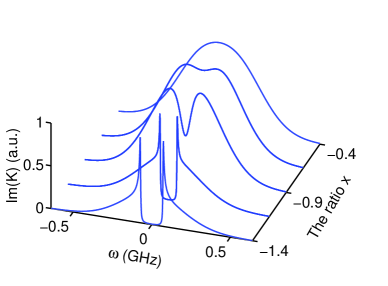
Figure 2: (Color online) The probe-field absorption spectrum Im($K$) of the ladder-I system as a function of $\omega$ and the wavenumber ratio $x$.

the numerical result of Im($K$) as a function of $\omega$ and $x$. The system parameters are chosen as $\Gamma_{2}=6$ MHz, $\Gamma_{3}=1$ MHz, $\gamma=0.5$ MHz, $\gamma_{ij}^{\rm col}=1$ MHz, and $\Omega_{a}=80$ MHz. We see that Im($K$) undergoes a transition from a deep, wide transparency window (doublet) to a single absorption peak when $x$ changes from $-1.4$ to $-0.4$. Since Fig. 2 is obtained by a numerical calculation, it is not easy to get a clear and definite conclusion on the quantum interference characters of the system. Thus we turn to an analytical approach by using the method developed in Refs. Agarwal1997 ; Anisimov2008 ; Tony2010 ; Anisimov2011 ; tan2013 ; Zhu2013 .

III.2 EIT-ATS crossover in hot Rubidium atomic gases

In many experimental studies on EIT or EIT-related effects in the ladder-I system with Doppler broadening, the excitation scheme $5S_{1/2}\rightarrow 5P_{3/2}\rightarrow 5D_{5/2}$ of ⁸⁷Rb atoms was adopted, such as did in Refs. Julio1995 ; Moon . In this situation, the wavenumber ratio $x=-1$, and the integration in Eq. (7) can be carried out analytically by using the residue theorem when the Maxwellian velocity distribution is replaced by the modified Lorentzian velocity distribution $f(v)=v_{T}/\left[\sqrt{\pi}(v^{2}+v_{T}^{2})\right]$. Such technique has been widely employed by many authors tan2013 ; Zhu2013 ; Elena2002 ; Lee2003 ; LiHuang2010 .

Note that the integrand in the second term of the Eq. (7) has only one pole $k_{b}v=-ik_{b}v_{T}=-i\Delta\omega_{D}$ in the lower half complex plane of $v$. Considering the contour integration shown in Fig. 3(a)

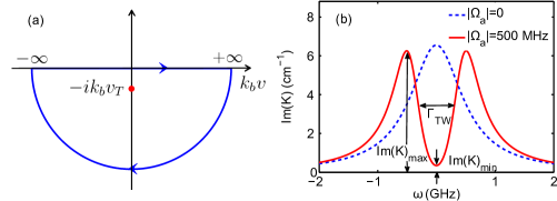
Figure 3: (Color online) (a) The pole $(0,-ik_{b}v_{T})$ of the integrand in Eq. (7) in the lower half complex plane of $v$. The closed curve with arrows is the contour chosen for calculating the integration in Eq. (7) by using the residue theorem. (b) Probe-field absorption spectrum Im($K$) as a function of $\omega$ for the hot ladder-I system with wavenumber ratio $x=-1$. The solid (dashed) line is for $|\Omega_{a}|=500$ MHz ($|\Omega_{a}|=0$). Definitions of Im$(K)_{\rm min}$, Im$(K)_{\rm max}$, and the width of transparency window $\Gamma_{\rm TW}$ are indicated in the figure.

and using the residue theorem, we obtain the exact result

$$K(\omega)=\frac{\omega}{c}+\frac{\sqrt{\pi}\kappa_{12}(\omega+i\gamma_{31})}{|\Omega_{a}|^{2}-(\omega+i\gamma_{21}+i\Delta\omega_{D})(\omega+i\gamma_{31})},$$ (8)

with$\Delta_{2}=\Delta_{3}=0$. Explicit expression of $K(\omega)$ for nonvanishing $\Delta_{2}$ and $\Delta_{3}$ can also be obtained but lengthy and thus omitted here.

Fig. 3(b) shows the profile of Im($K$) as a function of $\omega$. The dashed (solid) line is for the case of $|\Omega_{a}|=0$ ($|\Omega_{a}|=500$ MHz) for $\Gamma_{2}=6$ MHz, $\Gamma_{3}=1$ MHz, $\gamma=0.5$ MHz, $\gamma_{jl}^{{\rm col}}=1$ MHz, $\Delta\omega_{D}=270$ MHz and $\kappa_{12}=1\times 10^{9}$ cm^-1s^-1, used in Ref. Julio1995 . We see that the probe-field absorption spectrum for $|\Omega_{a}|=0$ has only a single peak. However, a transparency window is opened for $\Omega_{a}=500$ MHz. The minimum (Im$(K)_{\rm min}$), maximum (Im$(K)_{\rm max}$), and width of transparency window ($\Gamma_{\rm TW}$) are defined in the figure.

Equation (8) can be written as the form

$$K(\omega)=\frac{\omega}{c}-\sqrt{\pi}\kappa_{12}\frac{\omega+i\gamma_{31}}{(\omega-\omega_{+})(\omega-\omega_{-})},$$ (9)

with

$$\omega_{\pm}=\frac{1}{2}\left\{-i(\gamma_{21}+\gamma_{31}+\Delta\omega_{D})\pm 2\left[|\Omega_{a}|^{2}-|\Omega_{\rm ref}|^{2}\right]^{1/2}\right\},$$ (10)

where

$$\Omega_{\rm ref}\equiv\frac{1}{2}(\gamma_{21}+\Delta\omega_{D}-\gamma_{31}).$$ (11)

In order to illustrate the quantum interference effect in a simple and clear way, we decompose Im$(K)$ for different $\Omega_{a}$ as follows.

(i). Weak control field region (i.e. $|\Omega_{a}|<\Omega_{\rm ref}\approx\Delta\omega_{D}/2$): Equation (9) can be written as

$$K(\omega)=\frac{\omega}{c}+\sqrt{\pi}\kappa_{12}\left(\frac{A_{+}}{\omega-\omega_{+}}+\frac{A_{-}}{\omega-\omega_{-}}\right),$$ (12)

where $A_{\pm}=\mp(\omega_{\pm}+i\gamma_{31})/(\omega_{+}-\omega_{-})$. Since in this region ${\rm Re}(\omega_{\pm})={\rm Im}(A_{\pm})=0$, we obtain

$${\rm Im}(K)=\sqrt{\pi}\kappa_{12}\left(\frac{B_{+}}{\omega^{2}+\delta_{+}^{2}}+\frac{B_{-}}{\omega^{2}+\delta_{-}^{2}}\right)\equiv L_{2}+L_{1},$$ (13)

with $\delta_{\pm}={\rm Im}(\omega_{\pm})$, $B_{\pm}=A_{\pm}\delta_{\pm}$, and $L_{1(2)}=\sqrt{\pi}\kappa_{12}B_{-(+)}/(\omega^{2}+\delta_{-(+)}^{2})$. Thus the probe-field absorption profile comprises two Lorentzians centered at $\omega=0$.

Shown in Fig. 4(a)

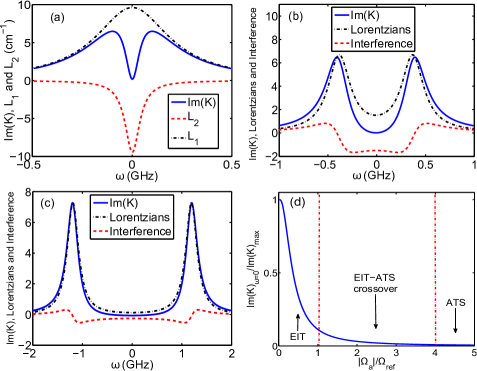
Figure 4: (Color online) EIT-ATS crossover for hot ladder-I system. (a) Probe-field absorption spectrum Im($K$) (solid line) in the region $|\Omega_{a}|<\Omega_{\rm ref}$ is a superposition of the positive $L_{1}$ (dash-dotted line) and the negative $L_{2}$ (dashed line). (b) Im($K$) (solid line) composed by two Lorentzians (dashed-dotted line) and destructive interference (dashed line) in the region $|\Omega_{a}|>\Omega_{\rm ref}$. (c) Im($K$) (solid line) composed by two Lorentzians (dashed-dotted line) and destructive interference (dashed line) in the region $|\Omega_{a}|>\Omega_{\rm ref}$. Panels (a), (b) and (c) correspond to EIT, EIT-ATS crossover, and ATS, respectively. (d) The “phase diagram” of ${\rm Im}(K)_{\omega=0}/{\rm Im}(K)_{\rm max}$ as a function of $|\Omega_{a}|/\Omega_{\rm ref}$ illustrating the transition from EIT to ATS for the hot ladder-I system. Three regions (EIT, EIT-ATS crossover, and ATS) are divided by two vertical dashed-dotted lines.

are the results of $L_{1}$, which is a positive single peak (the dash-dotted line), and $L_{2}$, which is a negative single peak (the dashed line). When plotting the figure, we have taken $\Omega_{a}=100$ MHz and the other parameters are the same as those used in Fig. 3(b). The superposition of $L_{1}$ and $L_{2}$ gives Im($K$) (the solid line), which displays a absorption doublet with a transparency window near at $\omega=0$. Because there exists a destructive interference between the positive $L_{1}$ and the negative $L_{2}$ in the probe-field absorption spectrum, the phenomenon found here belongs to EIT based on the criterion given in Refs. Anisimov2008 ; Tony2010 ; Anisimov2011 .

(ii). Intermediate control field region (i.e. $|\Omega_{a}|>\Omega_{\rm ref}$): In this region ${\rm Re}(\omega_{\pm})\neq 0$, we obtain

$$K(\omega)=\frac{\omega}{c}-\sqrt{\pi}\kappa_{12}\left[\frac{\omega+iW}{(\omega+iW-\delta)(\omega+iW+\delta)}+\frac{i(\gamma_{31}-W)}{(\omega+iW-\delta)(\omega+iW+\delta)}\right].$$ (14)

where $W\equiv(\gamma_{21}+\gamma_{31}+\Delta\omega_{D})/2$ and $\delta\equiv\sqrt{4|\Omega_{a}|^{2}-(\gamma_{21}+\Delta\omega_{D}-\gamma_{31})^{2}}/2$. The imaginary part of the Eq. (14) is given by

$${\rm Im}(K)= \frac{\sqrt{\pi}\kappa_{12}}{2}\left\{\frac{W}{(\omega-\delta)^{2}+W^{2}}+\frac{W}{(\omega+\delta)^{2}+W^{2}}\right.$$ (15)

$$\left.\hskip 19.91684pt+\frac{g}{\delta}\left[\frac{\omega-\delta}{(\omega-\delta)^{2}+W^{2}}-\frac{\omega+\delta}{(\omega+\delta)^{2}+W^{2}}\right]\right\},$$

with $g=W-\gamma_{31}$. The previous two terms (i.e. the two Lorentzian terms) in Eq. (15) can be thought of as the net contribution coming to the absorption from two different channels corresponding to the two dressed states created by the control field $\Omega_{a}$ Agarwal1997 . The following terms proportional to $g$ are clearly interference terms. The interference is controlled by the parameter $g$ and it is destructive (constructive) if $g>0$ ($g<0$). Since in the ladder-I system with $x=-1$, $g=(\gamma_{21}+\Delta\omega_{D}-\gamma_{31})/2$ is always positive, thus the quantum interference induced by the control field is always destructive.

Fig. 4(b) shows the probe-field absorption spectrum Im($K$) (solid line) as a function of $\omega$ for $|\Omega_{a}|>\Omega_{\rm ref}$. The dashed-dotted (dashed) line denotes the contribution by the two positive Lorentzians (negative interference terms). We see that the interference is destructive. The system parameters used are the same as those in Fig. 4(a) but with $\Omega_{a}=400$ MHz. A transparency window is opened due to the combined effect of EIT and ATS, which is deeper and wider than that in Fig. 4(a). We attribute such phenomenon as EIT-ATS crossover.

(iii). Large control field region (i.e., $|\Omega_{a}|\gg\Omega_{\rm ref}$): In this case, the quantum interference strength $g/\delta$ in Eq. (15) is very weak (i.e. $g/\delta\approx 0$). Im$(K)$ reduces to

$${\rm Im}(K)=\frac{\sqrt{\pi}\kappa_{12}}{2}\left[\frac{W}{(\omega-\delta)^{2}+W^{2}}+\frac{W}{(\omega+\delta)^{2}+W^{2}}\right].$$ (16)

Fig. 4(c) shows the result of the probe-field absorption spectrum as a function of $\omega$ for $|\Omega_{a}|\gg\Omega_{\rm ref}$. The dashed-dotted line represents the contribution by the sum of the two Lorentzians. For illustration, we have also plotted the contribution from the small interference terms [neglected in Eq. (15) ], denoted by the dashed line. We see that the interference is still destructive but very small. The solid line is the curve of Im($K$), which has two resonances at $\omega\approx\pm\Omega_{a}$. Parameters used are the same as those in Fig. 4(a) and Fig. 4(b) but with $\Omega_{a}=1.2$ GHz. Obviously, the phenomenon found in this case belongs to ATS because the transparency window opened is mainly due to the contribution of the two Lorentzians.

From the results given above, we see that the probe-field absorption spectrum experiences a transition from EIT to ATS as the control field is changed from small to large values. From the above result we can distinguish three different regions, i.e. the EIT ($|\Omega_{a}|<\Omega_{\rm ref}$), the EIT-ATS crossover ($1<|\Omega_{a}|/\Omega_{\rm ref}\leq 4$), and ATS $(|\Omega_{a}|/\Omega_{\rm ref}>4$). Fig. 4(d) shows a “phase diagram” that illustrates the transition from the EIT to ATS by plotting ${\rm Im}(K)_{\omega=0}/{\rm Im}(K)_{\rm max}$ as a function of $|\Omega_{a}|/\Omega_{\rm ref}$. Note that we have defined ${\rm Im}(K)_{\omega=0}/{\rm Im}(K)_{\rm max}=0.01$ as the border between EIT-ATS crossover and ATS regions. Our results on the characters of the quantum interference effect in the hot Rubidium atomic gases are consistent with those obtained in the experiments Julio1995 ; Moon . According to our analysis, the experiments carried out in Refs. Julio1995 ; Moon are mainly in the EIT region. We expect the EIT-ATS crossover and ATS may be observed experimentally if $\Omega_{a}$ is increased to the intermediate and the large control-field regions.

III.3 EIT-ATS crossover in hot molecular gases

In 2008, Lazoudis et al. Lazoudis2008 made an important experimental observation on EIT and ATS in a hot Na₂ molecular ladder-I system for the wavenumber ratio $x=-0.896$ and $x=-1.08$ note1 . Two excitation schemes of Na₂ molecules were adopted in Ref. Lazoudis2008 . The first (called the system B) is $X^{1}\sum_{g}^{+}(1,19)\rightarrow A^{1}\sum_{u}^{+}(3,18)\rightarrow 4^{1}\sum_{g}^{+}(0,17)$, and the second (called the system A) is $X^{1}\sum_{g}^{+}(0,19)\rightarrow A^{1}\sum_{u}^{+}(0,20)\rightarrow 2^{1}\Pi_{g}(0,19)$. Both of them correspond to the levels $|1\rangle\rightarrow|2\rangle\rightarrow|3\rangle$ in our Fig. 1(b). We now analyze this system by using the Eq. (7).

When $x$ is different from $-1$, the approach used in the last subsection is not easy to implement since the pole of the integrand in the Eq. (7) is not fixed in the lower (or upper) half complex plane of $v$. In this case, the value of the pole depends on both $x$ and $\omega$; moreover, it has an intersection with the real axis for $\omega=0$. As a result, the residue of the pole is a piecewise function, and the spectrum decomposition gives very complicated expressions not convenient for analyzing the quantum interference character of the system.

Because of the above mentioned difficulty, we turn to adopt the fitting method developed from the spectrum decomposition method, proposed by Anisimov et al. Anisimov2011 . According to the spectrum-decomposition formulas (13) and (16), we expect: (i)if the probe-field absorption spectrum has a good fit to the function

$$A_{\rm EIT}=\frac{B_{+}^{2}}{\omega^{2}+\delta_{+}^{2}}-\frac{B_{-}^{2}}{\omega^{2}+\delta_{-}^{2}},$$ (17)

EIT dominates, where $B_{+},\delta_{+},B_{-},\delta_{-}$ are fitting parameters; (ii)if the absorption spectrum has a good fit to the function

$$A_{\rm ATS}=C\left[\frac{1}{(\omega-\delta)^{2}+W^{2}}+\frac{1}{(\omega+\delta)^{2}+W^{2}}\right],$$ (18)

ATS dominates, with $C,\delta,W$ being fitting parameters.

Based on such technique, we find that EIT, ATS, and EIT-ATS crossover exist in the open molecular ladder-I system for both $x=-1.08$ and $x=-0.896$. Fig. 5(a) shows

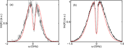
Figure 5: (Color online) The probe absorption spectrum Im($K$) as a function of $\omega$ for (a) $x=-0.896$ and $\Omega_{a}=265$ MHz (corresponding to system B of Ref. Lazoudis2008 ), and (b) $x=-1.08$ and $\Omega_{a}=242.5$ MHz (corresponding to system A of Ref. Lazoudis2008 ). The red dashed lines are our theoretical results, and the black-solid lines are the experimental ones from Ref. Lazoudis2008 .

the probe-field absorption spectrum Im($K$) for $x=-0.896$ and $\Omega_{a}=265$ MHz (corresponding to system B in Ref. Lazoudis2008 ). The black solid line is the experimental result from Ref. Lazoudis2008 , while the red dashed line is given by our theoretical calculation. The system parameters are given by $\Gamma_{12}=\Gamma_{42}=4.0\times 10^{7}$ $\mathrm{s}^{-1}$, $\Gamma_{23}=5.6\times 10^{6}$ $\mathrm{s}^{-1}$, $\Gamma_{53}=5.0\times 10^{7}$ $\mathrm{s}^{-1}$, $\gamma=2.7\times 10^{5}$ $\mathrm{s}^{-1}$, $\gamma_{jl}^{{\rm col}}=1\times 10^{6}$ $\mathrm{s}^{-1}$, and $\Delta\omega_{D}=5\times 10^{8}$ $\mathrm{s}^{-1}$. We see that our theoretical result agrees well with the experimental one. Note that the value of the reference Rabi frequency $\Omega_{\rm ref}$ is a function of the wavenumber ratio $x$. When $x=-0.896$, one has $\Omega_{\rm ref}\simeq 400$ MHz. Thus the system is in the weak control field region and the phenomenon found belongs to the EIT. Note in passing that here we have plotted the quantity Im$(K)$ which is proportional to the fluorescence intensity related to state $|2\rangle$ because $\sigma_{22}\simeq 2|\Omega_{b}|^{2}{\rm Im}(K)/\Gamma_{2}$.

Shown in Fig. 5(b) is the absorption spectrum Im($K$) for $x=-1.08$ and $\Omega_{a}=242.5$ MHz (corresponding to system A in Ref. Lazoudis2008 ). The system parameters are the same as that in Fig. 5(a). We see that our result also agrees well with the experimental one. Since in this case $\Omega_{\rm ref}\approx 150$ MHz, the system is in the intermediate control field region and hence the phenomenon found belongs to the EIT-ATS crossover. Note that there is a small difference for the width of the EIT transparency window between our result and that in the experiment Lazoudis2008 . The reason is mainly due to the approximation using the modified Lorentzian velocity distribution to replace the Maxwellian velocity distribution.

III.4 EIT in hot Rydberg atomic gases

Recently, much interest has focused on the EIT in hot Rydberg atomic gases due to its promising applications for storing, manipulating quantum information and precision spectroscopy saf ; moh1 ; moh2 ; wea ; rai ; pri ; pri1 ; sevi ; Lazoudis2008 ; Yang1997 ; Yong1995 ; Julio1995 ; Lee2000 ; Jason2001 ; Qi2002 ; Ahmed2006 ; Ahmed2007 ; Ray2007 ; Moon ; Kubler2010 ; gor ; petro ; ate . The ladder-I system has been widely adopted in the experimental study of Rydberg EIT, in which the transition is $5S_{1/2}\rightarrow 5P_{3/2}\rightarrow nD_{5/2}$ of ⁸⁵Rb atoms with $n$ being a large integer number. In this case, the upper state $|3\rangle$ in Fig. 1(c) is a Rydberg state. If the density (e.g. lower than $10^{8}$ cm^-3) of a Rydberg gas is low, the interaction between Rydberg atoms can be ignored. Our theory developed in Sec. II and Sec. III.1 can be applied to study the probe-field propagation in such system.

Shown in Fig. 6(a)

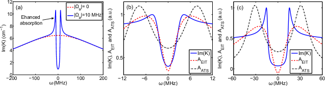
Figure 6: (Color online) (a) Probe-field absorption spectrum Im($K$) as a function of $\omega$. The blue solid (red dashed) line is for $|\Omega_{a}|=10$ MHz ($|\Omega_{a}|=0$). (b) Im($K$) (blue solid line), $A_{\rm EIT}$ (red dashed line) and $A_{\rm ATS}$ (black dashed-dotted line) as a function of $\omega$ for the weak control-field $\Omega_{a}=3$ MHz where $A_{\rm EIT}$ has a good fit. (c) The case for the intermediate control field $\Omega_{a}=15$ MHz where both $A_{\rm EIT}$ and $A_{\rm ATS}$ have poor fit.

is the numerical result of the probe-field absorption spectrum Im($K$) as a function of $\omega$ for the hot ladder-I system with wavenumber ratio $x=-1.63$, which corresponds to the experiment carried out in 2007 moh1 by Mohapatra et al. The red dashed (blue solid) line is for the case of $|\Omega_{a}|=0$ ($|\Omega_{a}|=10$ MHz) for the system parameters $\Gamma_{2}=6$ MHz, $\Gamma_{3}=1$ kHz, $\gamma_{jl}^{{\rm col}}=1$ MHz, $\Delta\omega_{D}=270$ MHz, and $\kappa_{12}=1\times 10^{9}$ cm^-1s^-1. We find that the line shape of Im($K$) displays enhanced absorption on both sides of the transparency window. This effect arises due to the wavelength mismatch between the control and probe fields combined with the effect of Doppler broadening. We now analyze the quantum interference character of such system.

Since the spectrum decomposition method is not convenient for the analysis for the case $x\neq-1$, we employ the fitting method as done in the last subsection. Shown in Fig. 6(b) and Fig. 6(c) are the results of Im($K$) (blue solid line), $A_{\rm EIT}(B_{+},\delta_{+},B_{-},\delta_{-})$ (red dashed line) and $A_{\rm ATS}(C,\delta,W)$ (black dash-dotted line) as a function of $\omega$ for $\Omega_{a}=3$ MHz and 15 MHz, respectively. The expressions of $A_{\rm EIT}$ and $A_{\rm ATS}$ have been given by Eqs. (17) and (18). From Fig. 6(b) we see that Im($K$) has a good fit to $A_{\rm EIT}(3.04,1.58,0.0381,0.208)$ and a poor fit to $A_{\rm ATS}(0.237,0.686,0.513)$. Thus EIT occurs in this weak control field region. However, for intermediate and large control field one can not find out the fitting parameters by which $A_{\rm EIT}$ and $A_{\rm ATS}$ can have a good fit to Im($K$) (Fig. 6(c) shows the result for $\Omega_{a}=15$ MHz). Consequently, based on the criterion of Ref. Anisimov2011 , neither EIT nor ATS dominates in the intermediate large control field regions.

Note that in the system discussed here the probe-field absorption spectrum Im($K$) doesn’t possess standard Lorentzian lineshape for large control field, which is due to the enhanced absorption by the Doppler effect and by the large wavenumber mismatch between the probe and control fields. Experimentally, EIT in hot Rydberg atomic gases has been observed in Ref. moh1 . Our theoretical result given above agrees with the experimental one. We hope that the theoretical result for the intermediate and large control field region predicted here may be verified experimentally in near future.

IV Quantum interference character of ladder-II system

If the probe field and the control field in the ladder-I system are exchanged, we obtain the ladder-II system (Fig. 1(b) with $\omega_{b}=\omega_{c}$, $\omega_{a}=\omega_{p}$). In this case, the Maxwell Eq. (3) under the SVEA is reduced to

$$i\left(\frac{\partial}{\partial z}+\frac{1}{c}\frac{\partial}{\partial t}\right)\Omega_{a}+\kappa_{23}\int_{-\infty}^{\infty}dvf(v)\sigma_{32}(v)=0,$$ (19)

with $\kappa_{23}={\cal N}\omega_{a}|\bm{\mu}_{32}|^{2}/(2\hbar\varepsilon_{0}c)$.

IV.1 Linear dispersion relation

The base state solution of the MB Eqs. (2) and (19) of the ladder-II system reads

$$\sigma_{11}^{(0)}=\left(\gamma\Gamma_{2}|d_{21}|^{2}+2\gamma\gamma_{21}|\Omega_{b}|^{2}\right)\frac{1}{D_{1}},$$ (20a)

$$\sigma_{22}^{(0)}=2\gamma\gamma_{21}|\Omega_{b}|^{2}\frac{1}{D_{1}},$$ (20b)

$$\sigma_{44}^{(0)}=2\gamma_{21}\Gamma_{42}|\Omega_{b}|^{2}\frac{1}{D_{1}},$$ (20c)

$$\sigma_{21}^{(0)}=-\gamma\Gamma_{2}\Omega_{b}d_{21}^{*}\frac{1}{D_{1}},$$ (20d)

and $\sigma^{(0)}_{31}=\sigma^{(0)}_{32}=\sigma^{(0)}_{33}=\sigma^{(0)}_{55}=0$, with $D_{1}\equiv\gamma\Gamma_{2}|d_{21}|^{2}+2\gamma_{21}(2\gamma+\Gamma_{42})|\Omega_{b}|^{2}$.

By using the same method as in Sec. III.1, one can obtain the solution of the MB Eqs. (2) and (19) in linear regime, with the linear dispersion relation given by

$$K(\omega)=\frac{\omega}{c}+\kappa_{23}\int_{-\infty}^{\infty}dvf(v)\frac{(\omega+d_{31})2\gamma\gamma_{21}|\Omega_{b}|^{2}-\gamma\Gamma_{2}|\Omega_{b}|^{2}d_{21}^{*}}{D_{1}\left[|\Omega_{b}|^{2}-(\omega+d_{31})(\omega+d_{32})\right]}.$$ (21)

Fig. 7 shows

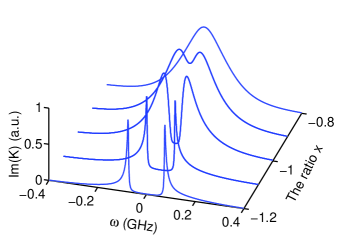
Figure 7: (Color online) The probe-field absorption spectrum Im($K$) of the ladder-II system as a function of $\omega$ and the wavenumber ratio $x=k_{a}/k_{b}$.

the probe-field absorption spectrum Im($K$) as a function of $\omega$ and the wavenumber ratio $x$. We see that, similar to the ladder-I system (Fig. 2), Im($K$) undergoes also a transition from a wide transparency window in the line center to a single absorption peak when $x$ changes from $-1.2$ to $-0.8$. The system parameters have been chosen as $\Gamma_{2}=6$ MHz, $\Gamma_{3}=1$ MHz, $\gamma=0.5$ MHz, $\gamma_{ij}^{\rm col}=1$ MHz, and $\Omega_{b}=100$ MHz.

IV.2 EIT-ATS crossover in hot Sodium atomic gases

In 1978, Gray and Stroud Gray1978 made an experimental observation on ATS in a ladder-II type hot sodium atomic system with $|1\rangle=|3S_{1/2},F=2,M_{F}=2\rangle$, $|2\rangle=|3P_{3/2},F=3,M_{F}=3\rangle$, $|3\rangle=4D_{5/2},F=4,M_{F}=4\rangle$, and the wavenumber ratio $x\approx-1$. Such system can be described by the MB Eqs. (2) and (19), and hence the linear dispersion relation (21) can be used to describe the probe-field propagation.

To get an analytical insight, we replace the Maxwellian velocity distribution by the modified Lorentzian velocity distribution and calculate the integration (21) using the residue theorem. We find two poles of the integrand in the lower half complex plane of $v$, which are $k_{a}v=-ik_{a}v_{T}=-i\Delta\omega_{D}$ and $k_{a}v=-iC=-i[\gamma_{21}^{2}+2\gamma_{21}(2\gamma+\Gamma_{42})|\Omega_{b}|^{2}/\gamma\Gamma_{2}]^{1/2}$. By taking the contour consisting of the lower half complex plane of $v$ and its real axis, we can calculate the integration exactly, with the result given by

$$K(\omega)=\omega/c+{\cal K}_{1}+{\cal K}_{2},$$ (22)

with

$${\cal K}_{1}=\frac{2\sqrt{\pi}\kappa_{23}\gamma_{21}|\Omega_{b}|^{2}\left\{\omega+i[\gamma_{31}+\Gamma_{2}(\Delta\omega_{D}+\gamma_{21})/(2\gamma_{21})]\right\}}{\Gamma_{2}(C^{2}-\Delta\omega_{D}^{2})\left[|\Omega_{b}|^{2}-(\omega+i\gamma_{31})(\omega+i\gamma_{32}+i\Delta\omega_{D})\right]},$$ (23a)

$${\cal K}_{2}=\frac{2\sqrt{\pi}\kappa_{23}\gamma_{21}\Delta\omega_{D}|\Omega_{b}|^{2}\left\{\omega+i[\gamma_{31}+\Gamma_{2}(C+\gamma_{21})/(2\gamma_{21})]\right\}}{\Gamma_{2}C(\Delta\omega_{D}^{2}-C^{2})\left[|\Omega_{b}|^{2}-(\omega+i\gamma_{31})(\omega+i\gamma_{32}+iC)\right]}.$$ (23b)

We can also carry out a spectrum decomposition for ${\cal K}_{j}$ ($j=1,2$), like that done in Ref. III.1. The explicit expressions of the decomposition have been given in Appendix A. Similarly, three different control field regions (i.e. the weak control field region $|\Omega_{b}|<\Omega_{\rm ref}$, the intermediate control field region $|\Omega_{b}|>\Omega_{\rm ref}$, and the strong control field region $|\Omega_{b}|\gg\Omega_{\rm ref}$; $\Omega_{\rm ref}\equiv\Delta\omega_{D}/2$) can also be obtained.

Fig. 8(a)

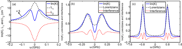
Figure 8: (Color online) EIT-ATS crossover for the hot atoms in the ladder-II system for the wavenumber ratio $x=-1$. (a) Probe-field absorption spectrum Im($K$) in the weak control field region ($|\Omega_{a}|<\Omega_{\rm ref}$). The dashed-dotted line is the contribution by positive $L_{1}$, the dashed line is by negative $L_{2}$. The sum of $L_{1}$ and $L_{2}$ gives Im($K$) (solid line). (b) Probe-field absorption spectrum Im($K$) (solid line) composed by two Lorentzians (dashed-dotted line) and the destructive interference (dashed line) in the intermediate control field region $|\Omega_{a}|>\Omega_{\rm ref}$. (c) Probe-field absorption spectrum Im($K$) (solid line) composed by two Lorentzians (dashed-dotted line) and the destructive interference (dashed line) in the strong control field region $|\Omega_{a}|\gg\Omega_{\rm ref}$. Panels (a), (b) and (c) correspond to EIT, EIT-ATS crossover, and ATS, respectively.

shows the absorption spectrum Im($K$) in the weak control field region ($|\Omega_{b}|=100$ MHz, which is smaller than $\Omega_{\rm ref}=150$ MHz). The dashed-dotted line is the contribution by positive $L_{1}$, and the dashed line is by negative $L_{2}$. The superposition (sum) of $L_{1}$ and $L_{2}$ gives Im($K$) (solid line). The expressions of $L_{1}$ and $L_{2}$ have been presented in Appendix A. System parameters are chosen as $\Gamma_{2}=10$ MHz, $\Gamma_{3}=3.15$ MHz, $\Delta\omega_{D}=300$ MHz Stroud96 , with other parameters the same as those in the last section. We see that in the curve of Im($K$) a deep transparency window is opened, resulting from the destructive quantum interference (because $L_{1}$ is positive and $L_{2}$ is negative). Hence in this region EIT exists.

Fig. 8(b) shows Im($K$) (solid line) in the intermediate control field region ($|\Omega_{b}|=200$ MHz), which is the sum of the two Lorentzians (dashed-dotted line) and the destructive interference (dashed line). In this region, a large dip appears in Im($K$) due to the contribution of the destructive interference. This region belongs to an EIT-ATS crossover.

Fig. 8(c) illustrates Im($K$) (solid line), the two Lorentzians (dashed-dotted line), and the destructive interference (dashed line) in the large control field region ($|\Omega_{b}|=800$ MHz). We see that in this region the contribution of the quantum interference is too small to be neglected. Obviously, the phenomenon found in this situation belongs to ATS because the transparency window opened is mainly due to the contribution by the two Lorentzians.

From the above analysis, we see that EIT, EIT-ATS crossover, and ATS exist in the ladder-II system with the Doppler broadening for the wavenumber ratio $x=-1$. This is different from cold ladder-II systems where no EIT and thus EIT-ATS crossover exist Tony2010 . Although the experiment on ATS in a hot atomic system with the ladder-II configuration for $x=-1$ has been realized Gray1978 ; Stroud96 , it seems that up to now no experimental study has been carried out on EIT, and EIT-ATS crossover in the ladder-II system with Doppler broadening. We hope new experiments can be designed to verify our predictions given here.

IV.3 Microwave induced transparency

We now discuss the case when the control field in the ladder-II system is a microwave field, i.e. $x\rightarrow 0$. The relevant experimental result, named by Zhao et al. Yang1997 as microwave induced transparency, was first reported in 1997.

In this case, the level diagram and excitation scheme is given by Fig. 9,

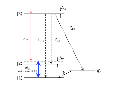
Figure 9: (Color online) Microwave field driven ladder-II configuration. All notations are given in the text.

in which the optical transition between the two lower states $|1\rangle$ and $|2\rangle$ is forbidden, but the optical transitions between the highest state $|3\rangle$ and the two lower states $|1\rangle$, $|2\rangle$ are allowed, so $\Gamma_{12}=\Gamma_{42}=0$. All spontaneous emission decay rates $\Gamma_{31}$, $\Gamma_{32}$, and $\Gamma_{34}$ (corresponding to the decay pathways $|3\rangle\rightarrow|1\rangle$, $|3\rangle\rightarrow|2\rangle$, and $|3\rangle\rightarrow|4\rangle$, respectively), and the transit rate $\gamma$ from $|4\rangle\rightarrow|3\rangle$ have been indicated in the figure.

The base state solution of the MB equations for the present case reads $\sigma_{11}^{(0)}=\sigma_{22}^{(0)}=1/2$ and other $\sigma_{jl}^{(0)}=0$. The linear dispersion relation of the system is given by

$$K(\omega)=\frac{\omega}{c}+\frac{\kappa_{23}}{2}\int_{-\infty}^{\infty}dvf(v)\frac{\omega+d_{31}}{|\Omega_{b}|^{2}-(\omega+d_{31})(\omega+d_{32})},$$ (24)

with $d_{31}=-k_{a}v+\Delta_{3}+i\gamma_{31}$. Because $\gamma_{31}=\gamma_{32}$, the integrand in Eq.(24) has only one pole in the lower half complex plane of $v$, given by $k_{a}v=-ik_{a}v_{T}=-i\Delta\omega_{D}$. When replacing the Maxwellian distribution by the modified Lorentzian distribution, the integration can be calculated exactly by using the residue theorem. One obtains

$$K(\omega)=\frac{\omega}{c}+\frac{\sqrt{\pi}\kappa_{23}}{2}\frac{\omega+i\gamma_{31}+i\Delta\omega_{D}}{|\Omega_{b}|^{2}-(\omega+i\gamma_{31}+i\Delta\omega_{D})^{2}}.$$ (25)

It is easy to get the probe-field absorption spectrum Im($K$) from Eq. (25), which reads

$${\rm Im}(K)=\frac{\sqrt{\pi}\kappa_{23}}{2}\left[\frac{W}{(\omega-\delta)^{2}+W^{2}}+\frac{W}{(\omega+\delta)^{2}+W^{2}}\right],$$ (26)

with $W=\gamma_{31}+\Delta\omega_{D}$ and $\delta=|\Omega_{b}|$. Equation (26) consists of two pure Lorentzians, which means that there is no quantum interference occurring in the system and the phenomenon found is an ATS one. Consequently, we conclude that there is no EIT and EIT-ATS crossover in the ladder-II system when the control field used is a microwave one.

V Summary

In Sec. III and Sec. IV, we have analyzed the quantum interference characters in the hot ladder-I and ladder-II systems with Doppler broadening for many different cases. For clearness and for comparison, in Table 1

Table 1: Quantum interference characters for various ladder systems with different wavenumber ratio $x$. “Hot” (“Cold”) means hot (cold) atoms or molecules. “Any” means any value of $x$. The last column gives some references in which related experiments have been carried out.

System	Wavenumber ratio $x$	EIT	ATS	Reference
Ladder-I (Hot)	$-0.896$	Yes	Yes	Lazoudis2008
	$-1$	Yes	Yes	Julio1995 ; Moon
	$-1.08$	Yes	Yes	Lazoudis2008
	$-1.63$	Yes	No	moh1
Ladder-II (Hot)	$-1$	Yes	Yes	Gray1978
	0	No	Yes	Yang1997
Ladder-I (Cold)	Any	Yes	Yes	Jason2001 ; Weatherill2008
Ladder-II (Cold)	Any	No	Yes	Teo2003 ; Hao2013

we have summarized the main results obtained for different ladder configurations with different wavenumver ratio $x$. The first four lines are for the hot ladder-I system; the next two lines are for the hot ladder-II system. The seventh and eighth lines are for cold ladder-I system and cold ladder-II system, for which relevant theoretical analysis has been given in Refs. Agarwal1997 ; Tony2010 and related experiments were made in Refs. Jason2001 ; Weatherill2008 ; Teo2003 ; Hao2013 . If in the table there is “Yes” in the same line for both EIT and ATS, an EIT-ATS crossover also exists in the system. The last column of the table gives some references in which related experimental results were reported.

In summary, in this work we have proposed a general theoretical scheme for studying the crossover from EIT to ATS in the open systems of ladder-type level configuration with Doppler broadening. We have elucidated various mechanisms of the EIT, ATS, and their crossover in such systems in a clear and unified way. We have obtained the following conclusions. First, when the wavenumber ratio $x\approx-1$, EIT, ATS, and EIT-ATS crossover exist for both ladder-I and ladder-II systems. Second, when $x$ is far from $-1$, EIT can occur but ATS is destroyed if the upper state of the ladder-I system is a Rydberg state. Third, ATS exists but EIT is not possible if the control field that couples the two lower states of the ladder-II system is a microwave field. Our theoretical analysis have applied to various ladder systems (including hot gases of Rubidium atoms, molecules, and Rydberg atoms, and so on), and the results obtained on the quantum interference characters agree well with experimental ones reported up to now. The results obtained here may have practical applications in optical information processing and transmission.

Appendix A Spectrum decomposition of the ladder-II system for the wavenumber ratio $x=-1$

${\cal K}_{j}$ $(j=1,2)$ in Eq. (23) can be decomposed as the form

$${\cal K}_{j}=\eta_{j}\left(\frac{A_{j+}}{\omega-\delta_{j+}}+\frac{A_{j-}}{\omega-\delta_{j-}}\right),$$ (27)

where $\eta_{j}$, $A_{j\pm}$ are constants, $\delta_{j+}$ and $\delta_{j-}$ are two spectrum poles of ${\cal K}_{j}$, given by

$$\eta_{1}=\frac{2\sqrt{\pi}\kappa_{23}\gamma_{21}|\Omega_{b}|^{2}}{\Gamma_{2}(C^{2}-\Delta\omega_{D}^{2})},$$ (28a)

$$\eta_{2}=\frac{2\sqrt{\pi}\kappa_{23}\gamma_{21}\Delta\omega_{D}|\Omega_{b}|^{2}}{\Gamma_{2}C(\Delta\omega_{D}^{2}-C^{2})},$$ (28b)

$$\delta_{1\pm}=\frac{1}{2}\left[-i(\gamma_{32}+\Delta\omega_{D}+\gamma_{31})\pm\sqrt{4|\Omega_{b}|^{2}-(\gamma_{32}+\Delta\omega_{D}-\gamma_{31})^{2}}\right],$$ (28c)

$$\delta_{2\pm}=\frac{1}{2}\left[-i(\gamma_{32}+C+\gamma_{31})\pm\sqrt{4|\Omega_{b}|^{2}-(\gamma_{32}+C-\gamma_{31})^{2}}\right],$$ (28d)

$$A_{1\pm}=\mp\left\{\delta_{1\pm}-\left[\gamma_{31}+\frac{\Gamma_{2}}{2\gamma_{21}}(\Delta\omega_{D}+\gamma_{21})\right]\right\}/(\delta_{1+}-\delta_{1-}),$$ (28e)

$$A_{2\pm}=\mp\left\{\delta_{2\pm}-\left[\gamma_{31}+\frac{\Gamma_{2}}{2\gamma_{21}}(C+\gamma_{21})\right]\right\}/(\delta_{2+}-\delta_{2-}).$$ (28f)

In order to illustrate the quantum interference effect in a simple and clear way, we decompose Im$({\cal K}_{j})$ in different control field regions as follows.

(i).Weak control field region (i.e. $|\Omega_{b}|<\Omega_{\rm ref}\approx\Delta\omega_{D}/2$): In this region, one has Re$(\delta_{j\pm})$=0, Im$(A_{j\pm})$=0, and hence

$${\rm Im}(K)=\sum_{j=1}^{2}{\rm Im}({\cal K}_{j})=\sum_{j=1}^{2}\eta_{j}\left(\frac{B_{j+}}{\omega^{2}+W_{j+}^{2}}+\frac{B_{j-}}{\omega^{2}+W_{j-}^{2}}\right)=L_{1}+L_{2},$$ (29)

where $L_{1}$ and $L_{2}$ are defined by

$$L_{1}=\frac{\eta_{1}B_{1-}}{\omega^{2}+W_{1-}^{2}}+\frac{\eta_{2}B_{2-}}{\omega^{2}+W_{2-}^{2}}$$ (30a)

$$L_{2}=\frac{\eta_{1}B_{1+}}{\omega^{2}+W_{1+}^{2}}+\frac{\eta_{2}B_{2+}}{\omega^{2}+W_{2+}^{2}},$$ (30b)

with the real constants

$$C_{j+}=-W_{j+}(W_{j+}+\Gamma^{w}_{j})/(W_{j+}-W_{j-}),$$ (31a)

$$C_{j-}=W_{j-}(W_{j-}+\Gamma^{w}_{j})/(W_{j+}-W_{j-}),$$ (31b)

$$W_{1\pm}=\frac{1}{2}\left[\gamma_{32}+\gamma_{31}+\Delta\omega_{D}\pm\sqrt{[\gamma_{32}+\Delta\omega_{D}-\gamma_{31}]^{2}-4|\Omega_{b}|^{2}}\right],$$ (31c)

$$W_{2\pm}=\frac{1}{2}\left[\gamma_{32}+\gamma_{31}+C\pm\sqrt{[\gamma_{32}+C-\gamma_{31}]^{2}-4|\Omega_{b}|^{2}}\right],$$ (31d)

$$\Gamma_{1}^{w}=\gamma_{31}+\frac{\Gamma_{2}}{2\gamma_{21}}(\Delta\omega_{D}+\gamma_{21}),$$ (31e)

$$\Gamma_{2}^{w}=\gamma_{31}+\frac{\Gamma_{2}}{2\gamma_{21}}(C+\gamma_{21}).$$ (31f)

(ii).Intermediate control field region (i.e. $|\Omega_{b}|>\Omega_{\rm ref}$): By extending the approach by Agarwal Agarwal1997 , we can decompose Im$({\cal K}_{j})$ ($j=1,2$) as the form

$${\rm Im}({\cal K}_{j})=\eta_{j} \left\{\frac{1}{2}\left[\frac{W_{j}}{(\omega-\delta_{j}^{r})^{2}+W_{j}^{2}}+\frac{W_{j}}{(\omega+\delta_{j}^{r})^{2}+W_{j}^{2}}\right]\right.$$ (32)

$$\left.+\frac{g_{j}}{2\delta_{j}^{r}}\left[\frac{\omega-\delta_{j}^{r}}{(\omega-\delta_{j}^{r})^{2}+W_{j}^{2}}-\frac{\omega+\delta_{j}^{r}}{(\omega+\delta_{j}^{r})^{2}+W_{j}^{2}}\right]\right\},$$

where

$$W_{1}=(\gamma_{31}+\gamma_{32}+\Delta\omega_{D})/2,$$ (33a)

$$W_{2}=(\gamma_{31}+\gamma_{32}+C)/2,$$ (33b)

$$\delta^{r}_{1}=\sqrt{4|\Omega_{b}|^{2}-(\gamma_{32}+\Delta\omega_{D}-\gamma_{31})^{2}}/2,$$ (33c)

$$\delta^{r}_{2}=\sqrt{4|\Omega_{b}|^{2}-(\gamma_{32}+C-\gamma_{31})^{2}}/2,$$ (33d)

$$g_{1}=-\frac{\Gamma_{2}}{4}+\frac{\gamma_{21}-\Gamma_{2}}{2\gamma_{21}}\Delta\omega_{D},$$ (33e)

$$g_{2}=-\frac{\Gamma_{2}}{4}+\frac{\gamma_{21}-\Gamma_{2}}{2\gamma_{21}}C.$$ (33f)

(iii).Large control field region (i.e. $|\Omega_{b}|\gg\Omega_{\rm ref}$): In this case, the quantum interference strength $g_{j}/\delta_{j}^{r}$ in Eq. (32) is very weak and negligible. We have

$${\rm Im}({\cal K}_{j})\approx\frac{\eta_{j}}{2}\left[\frac{W_{j}}{(\omega-\delta_{j}^{r})^{2}+W_{j}^{2}}+\frac{W_{j}}{(\omega+\delta_{j}^{r})^{2}+W_{j}^{2}}\right].$$ (34)

References

- (1) M. Fleischhauer, A. Imamoglu, and J. P. Marangos, Rev. Mod. Phys. 77, 633 (2005).
- (2) S. H. Autler and C. H. Townes, Phys. Rev. 100, 703 (1955).
- (3) C. Cohen-Tannoudji, in “Amazing Light: a volume dedicated to Charles Hard Townes on his 80th birthday”, edited by R. Y. Chiao, p. 109 (Springer, 1996).
- (4) G. S. Agarwal, Phys. Rev. A 55, 2467 (1997).
- (5) P. Anisimov and O. Kocharovskaya, J. Mod. Opt. 55, 3159 (2008).
- (6) T. Y. Abi-Salloum, Phys. Rev. A 81, 053836 (2010).
- (7) P. M. Anisimov, J. P. Dowling, and B. C. Sanders, Phys. Rev. Lett 107 , 163604 (2011).
- (8) L. Giner et al., Phys. Rev. A 87, 013823 (2013).
- (9) C. Tan, C. Zhu, and G. Huang, J. Phys. B: At. Mol. Opt. Phys. 46, 025103 (2013).
- (10) C. Zhu, C. Tan, and G. Huang, Phys. Rev. A 87, 043813 (2013).
- (11) In literature, the ladder system is also called cascade system by many authors, e.g. Tony2010 .
- (12) M. Saffman, T. G. Walker, and K. Mölmer, Rev. Mod. Phys. 82, 2313 (2010).
- (13) J. D. Pritchard, K. J. Weatherill, and C. S. Adams, arXiv: 1205.4890v1.
- (14) S. Sevincli et al., J. Phys. B 44, 184018 (2011).
- (15) A. K. Mohapatra, T. R. Jackson, and C. S. Adams, Phys. Rev. Lett. 98, 113003 (2007).
- (16) A. K. Mohapatra et al., Nature Phys. 4, 890 (2008).
- (17) K. J. Weatherill et al., J. Phys. B 41, 201002 (2008).
- (18) U. Raitzsch et al., New J. Phys. 11, 055014 (2009).
- (19) J. D. Pritchard et al., Phys. Rev. Lett. 105, 193603 (2010).
- (20) A. Lazoudis et al., Phys. Rev. A 78, 043405 (2008).
- (21) Y. Zhao et al., Phys. Rev. Lett 79, 641 (1997).
- (22) Y.-q. Li and M. Xiao, Phys. Rev. A 51, 4959 (1995).
- (23) J. Gea-Banacloche et al., Phys. Rev. A 51, 579 (1995).
- (24) H. Lee, Y. Rostovtsev, and M. O. Scully, Phys. Rev. A 62, 063804 (2000).
- (25) J. J. Clarke, W. A. van Wijngaarden, and H. Chen, Phys. Rev. A 64, 023818 (2001).
- (26) J. Qi et al., Phys. Rev. Lett 88, 173003 (2002).
- (27) E. Ahmed et al., J. Chem. Phys. 124, 084308 (2006).
- (28) E. Ahmed and A. M. Lyyra, Phys. Rev. A 76, 053407 (2007).
- (29) R.-Y. Chang et al., Phys. Rev. A 76, 053420 (2007).
- (30) H. S. Moon, L. Lee, and J. B. Kim, Opt. Express 16, 12163 (2008).
- (31) H. Kbler et al., Nature Photon. 4, 112 (2010).
- (32) A. V. Gorshkov et al., Phys. Rev. Lett. 107, 133602 (2011).
- (33) D. Petrosyan, J. Otterbach, and M. Fleischhauer, Phys. Rev. Lett. 107, 213601 (2011).
- (34) C. Ates, S. Sevincli, and T. Pohl, Phys. Rev. A 83, 041802(R) (2011).
- (35) Y. O. Dudin, L. Li, F. Bariani, and A. Kuzmich, Nat. Phys. 8, 790 (12).
- (36) B. Huber et al., Phys. Rev. Lett 107, 243001 (2011).
- (37) H. Schempp et al., Phys. Rev. Lett 104, 173602 (2010).
- (38) T. Peyronel et al., Nature 488, 57 (2012).
- (39) F. Bariani et al., Phys. Rev. Lett 108, 030501 (2012).
- (40) J. A. Sedlacek et al., Nat. Phys. 8, 819 (2012).
- (41) E. Kuznetsova et al., Phys. Rev. A 66, 063802 (2002).
- (42) H. Lee et al., Appl. Phys. B 76, 33 (2003).
- (43) L. Li and G. Huang, Phys. Rev. A 82, 023809 (2010).
- (44) Note that the wavenumber ratio defined in our paper is the reciprocal of that defined in Ref. Lazoudis2008 .
- (45) H. R. Gray and C. R. Stroud Jr., Opt. Commun. 25, 359 (1978).
- (46) S. Papademetriou, M. F. Van Leeuwen, and C. R. Stroud, Jr., Phys. Rev. A 53, 997 (1996).
- (47) K. J. Weatherill et al., J. Phys. B: At. Mol. Opt. Phys. 41, 201002 (2008).
- (48) B. K. Teo et al., Phys. Rev. A 68, 053407 (2003).
- (49) H. Zhang et al., Phys. Rev. A 87, 033835 (2013).