SPH Entropy Errors and the Pressure Blip

Abstract

The spurious pressure jump at a contact discontinuity, in SPH simulations of the compressible Euler equations is investigated. From the spatiotemporal behaviour of the error, the SPH pressure jump is likened to entropy errors observed for artificial viscosity based finite difference/volume schemes. The error is observed to be generated at start-up and dissipation is the only recourse to mitigate it’s effect.
We show that similar errors are generated for the Lagrangian plus remap version of the Piecewise Parabolic Method (PPM) finite volume code (PPMLR). Through a comparison with the direct Eulerian version of the PPM code (PPMDE), we argue that a lack of diffusion across the material wave (contact discontinuity) is responsible for the error in PPMLR. We verify this hypothesis by constructing a more dissipative version of the remap code using a piecewise constant reconstruction. As an application to SPH, we propose a hybrid GSPH scheme that adds the requisite dissipation by utilizing a more dissipative Riemann solver for the energy equation. The proposed modification to the GSPH scheme, and it’s improved treatment of the anomaly is verified for flows with strong shocks in one and two dimensions.
The result that dissipation must act across the density and energy equations provides a consistent explanation for many of the hitherto proposed “cures” or “fixes” for the problem.

1 Introduction

SPH solutions to the compressible Euler equations are characterized by an anomalous “blip” or kink in the pressure at the contact discontinuity. The density profile is accurate which means the internal energy shows a corresponding heating/cooling to mirror the pressure jump. The error, once introduced, neither grows nor attenuates without dissipation and is simply advected with the particles at the local material velocity. Monaghan and Gingold [1] were the first to observe this behaviour when they applied SPH to simulate shock-tube problems. Their observations lead them to ascribe the phenomenon to general “starting” errors when discontinuous initial profiles are used. Presumably, SPH struggles with the discontinuous thermal energy. Resolving this behaviour has been the focus of numerous researchers over the last thirty years as this is manifestly a grave drawback of the method. Despite this error, SPH has been found to be useful within the astrophysics community, it’s application often preceded by “code-comparisons” with existing Eulerian techniques. One of the early comparisons was undertaken by Davies et al. [2], who compared SPH simulations of stellar collisions with the Piecewise Parabolic Method (PPM). They suggest that the advantages of each approach are mutually exclusive, although the two approaches were qualitatively similar. Caution is advised in extending this observation for other calculations in which different hydrodynamic effects determine the solution. About the same time, Steinmetz and Müller [3] had also suggested that SPH and finite difference methods should be looked upon as complimentary methods to solve hydrodynamic problems. In their seminal work, Agertz et al. [4] performed a comprehensive comparison of astrophysical codes (using GADGET [5] for SPH) for the simulation of interacting multi-phase fluids. The un-physical pressure jump at a density gradient, as produced by SPH in it’s standard formulation was found to render the method incapable of resolving hydrodynamic instabilities like the Kelvin-Helmholtz (KHI) or Rayleigh-Taylor instabilities (RTI). A similar comparison was carried out by Tasker et al. [6] for test problems with analytical solutions, therefore enabling a more quantitative comparison. While SPH was found to be generally comparable in it’s accuracy with the Eulerian schemes, a major difference was the pressure jump at the contact discontinuity, which is absent for grid-based codes. For the hydrodynamics of multi-phase fluids (more generally at a density gradient), this spurious pressure jump behaves like an artificial surface tension force, inhibiting the development of density driven instabilities like KHI. In another study, Okamoto et al. [7] observed that the erroneous pressure jump can also result in spurious momentum transfer across shearing flows, significantly affecting numerical results. These code comparisons rekindled the need to resolve the spurious pressure at the contact discontinuity, with the Kelvin-Helmholtz instability (KHI) often used as a canonical “mixing” problem exposing the method’s vulnerability.
Among the many tricks for SPH [8], arguably the oldest one is a judicious use of artificial dissipation. Thermal conduction is as old as artificial viscosity itself with Monaghan [9] and Brookshaw [10] being early advocates for it’s use in treating “wall-heating” errors. It has been used for example, by Sigalotti et al. [11, 12] and Rosswog and Price [13] for strong shock problems in hydrodynamics and magnetohydrodynamics respectively. Addressing the mixing problem originally highlighted by Agertz et al. [4], Price [14] demonstrated that a judicious use of thermal conduction enables a suitable description of density driven instabilities like KHI. The conduction terms are formulated using the signal-based artificial viscosity [15] and are constructed to result in a diffusion of energy across the contact discontinuity. The use of and need for similar thermal conduction terms was also suggested by Wadsley et al. [16], García-Senz et al. [17] and and Valcke et al. [18] for mixing problems in astrophysics. Some authors also suggest that apart from the use of the thermal conduction, the magnitude of the pressure jump can be curtailed by relaxing the initial conditions and by using a modified kernel with an increased sampling. Thermal conduction is necessary for the long term simulation and to avoid “oily” [18] or “gloopy” [19] features in the solution. Following Price, Valdarnini [20], Kawata et al. [21] and Rosswog [22] have also advocated the use of artificial thermal conduction. By using an error and stability analysis, Read et al. [19] showed that the inability of SPH to adequately resolve mixing was due in part to a “Local Mixing Instability” (LMI), whereby, particles are inhibited to mix on the kernel scale due to entropy conservation, which in turn results in a pressure discontinuity. The LMI is therefore another term for the pressure “blip” in the context of hydrodynamic mixing. The LMI was cured by using a modified density estimate, similar to that employed by Ritchie and Thomas [23], to ensure a single valued pressure throughout the flow. The modified density approaches ([23, 24, 19]) are designed for a more accurate density estimation for multi-phase fluids (mixing problems) in pressure equilibrium. Consequently, they perform poorly for flows with strong shocks. Indeed, in a recent article, Read and Hayfield [25] discuss a new high-order dissipation switch for adaptive viscosity in which they forgo the modified density approach in favour of an artificial heating term as proposed by Price [14].

Moving away from adding thermal conduction in a somewhat ad-hoc manner, Price [26] argues that the assumption of a differentiable density is the cause of the spurious pressure jump. The density estimate plays a central role in the variational formulation of SPH and is used to define an implicit particle volume through the ratio of particle mass to particle density. Saitoh and Makino [27] took cue from this idea to develop a density-independent SPH (DISPH) by replacing the mass density by an equivalent pressure density and it’s arbitrary function. Hopkins [28] also considered the idea of replacing the particle volume, traditionally defined by the mass density, by an arbitrary smoothed function. A family of equivalent Lagrangian schemes are derived by different choices of the function. In particular, the pressure-entropy formulation was shown to be superior at resolving mixing in the hydrodynamic context. However, there appear to be problems for shocked flows (due to the non-isentropic nature of the flow), similar to the modified density approach occurs for this formulation as well [29].

The SPH formulations discussed hitherto were of the variational kind with the use of explicit dissipation terms. Inutsuka [30] developed an artificial-viscosity free scheme that requires the solution of a Riemann problem between interacting particle pairs. The Riemann solver introduces the necessary and sufficient dissipation required to stabilize the scheme. Although the pressure blip is present for these Godunov SPH (GSPH) schemes, it is less pronounced. The result is a more suitable description of fluid instabilities like KHI. Indeed, Cha et al. [31] found GSPH to be superior to the standard SPH for the development of KHI. They argue in favour of the linear consistency in the GSPH momentum equation and a more accurate Lagrangian function used in GSPH. Murante et al. [32] observed similar advantages of GSPH for the simulation of hydrodynamical instabilities vis-a-vis standard SPH. Another artificial-viscosity free SPH scheme was proposed by Lanzafame [33] by considering shock flows as non-equilibrium events. The equation of state is reformulated according to a Riemann problem to introduce the necessary dissipation. Incidentally, these GodunovSPH schemes typically include an implicit thermal conduction term which is known ([14]) to ameliorate the pressure jump. Indeed, the authors have shown [34] that GSPH with a class of approximate Riemann solvers is essentially equivalent to the standard SPH with artificial viscosity and thermal conduction terms.

It is worth noting that despite the numerous efforts to address this pressure jump, the error is at best ameliorated, with it’s adverse effects kept to within acceptable limits. Care must be exercised with the use of thermal conduction so as to avoid excessive smearing and a resulting loss of accuracy. This is achieved through viscosity limiters [35, 25, 36, 26] and solution dependent conductivity coefficients [12, 26]. Without a unifying theory however, the different approaches seem serendipitous and somewhat ad-hoc. Success of a particular method notwithstanding, a discernible pattern among all proposed solutions is the introduction of a certain dissipation into the equations of motion to handle the pressure jump. The dissipation is introduced either in the form of an explicit ([37, 14, 26]) or implicit (GSPH) thermal conduction ([30, 31, 32]), or by more subtle means via the state equation [33], density estimate [19] or particle volume [27, 28].
That dissipation can be used to progressively smear the pressure blip once it is created should be fairly obvious. A more fundamental question that can be asked perhaps, pertains to the origin of this error. Towards this goal, we search for similar behaviour in finite difference/volume schemes. These grid-based schemes have received a great deal of attention and success within the CFD community and it is therefore helpful to study them. In particular, if we can relate the SPH errors to those generated with a suitable finite volume scheme, we can gain new insights and a more satisfying explanation as to why the aforementioned approaches work.

As it turns out, a pressure blip, exactly analogous to SPH, is produced when using the Lagrange plus Eulerian remap version of the PPM code, PPMLR [38, 39, 40]. Remap schemes involve a Lagrangian advection step in which the cells move, followed by a conservative remap onto the original Eulerian grid. We find (agreeing with the argument of Davies et al. [2]) it highly unlikely that two fundamentally different approaches result in the same erroneous features. Interestingly, the Eulerian version of the PPM (PPMDE) and indeed, other Eulerian schemes [41, 42] do not exhibit this anomaly. Lagrangian finite difference codes have traditionally fallen out in favour of their Eulerian counterparts and we are led to conjecture therefore that the difference between the two versions of the PPM scheme can provide an answer to origin of the pressure jump in SPH.

This work is outlined as follows. In Sec. 2, we use a one-dimensional shock tube problem to provide numerical evidence to the claim that PPMLR exhibits, qualitatively the same errors as the SPH pressure jump at the contact discontinuity. In Sec. 3, we use the spatiotemporal behaviour of the SPH error to draw an analogy with “wall-heating” errors for traditional finite difference schemes and argue that the pressure jump is a result of a spurious entropy generation in the initial transient phase of shock formation. In Sec. 4, through a comparison of PPMLR and PPMDE schemes, a lack of diffusion in the material wave (contact) is highlighted as the source of the error and we demonstrate how it may be eliminated for PPMLR by using a more diffusive Lagrangian advection step. Finally, in Sec. 5, we use these ideas to propose a minor modification to the GSPH scheme, where the requisite dissipation is added through a suitable choice of an approximate Riemann solver (similar to the method proposed by Shen et al. [43]). The scheme is applied to standard test problems in one and two dimensions to demonstrate it’s effectiveness in mitigating the pressure jump for flows with strong shocks. We summarize this work in Sec. 6, with conclusions drawn from this work and suggestions for possible extensions. All numerical results presented in this manuscript are generated using the code (SPH2D), which is freely available for validation and use.

2 Numerical evidence of the pressure blip

In this section, we provide numerical evidence for the existence of the pressure discontinuity when using SPH and the Lagrange plus remap version of the Piecewise Parabolic Method (PPMLR [38, 39]) finite difference code. The error is particularly severe for SPH and generally arises across a density gradient (contact discontinuity). We consider two one-dimensional shock tube problems that work well to highlight the anomalous behaviour. The initial conditions are defined with the the left (l) and right (r) states displayed in Table. 1

Test	$\rho_{l}$	$p_{l}$	$u_{l}$	$\rho_{r}$	$p_{r}$	$u_{r}$
Sod’s shock-tube	1	1	0	0.125	0.1	0
Blast-wave	1	1000	0	1	0.01	0

Table 1: Initial data for the test problems to highlight the pressure discontinuity

The first test is the famous Sod’s shock tube [44] problem. This test represents the bare minimum a numerical scheme for the compressible Euler equations should hope to resolve. The initial conditions result in a right moving contact discontinuity sandwiched between a left moving rarefaction and a right moving shock wave. The solution is self similar with four constant states separated by the three waves. The second test is a more stringent version, referred to as the blast-wave problem, in which the magnitude of the initial pressure jump ($p_{l}/p_{r}$) is $10^{5}$. The wave structure is similar with a strong, right facing shock wave ($M=198$) moving into the low pressure gas.
For the SPH results, we use our SPH2D [45] code that implements the variational formulation described by Price [26]. Thermal conduction is turned off for both test problems to highlight the errors at the contact discontinuity. For the PPMLR method, we have used John Blondin’s VH-1 [39] and Jim Stone’s CMHOG [40] codes independently to verify our results. Both codes implement the PPMLR algorithm proposed by Colella and Woodward [38].

2.1 Test $1$: Sod’s shock-tube problem

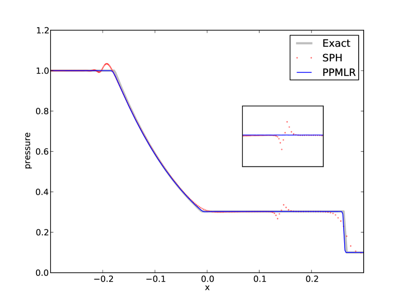
Figure 1: Numerical pressure for Sod’s shock-tube problem using SPH (dots), PPMLR (solid blue line) at $t=0.15s$, compared with the exact solution (solid black line). The pressure “blip” is clearly visible in the SPH solution at the contact $x\approx 0.17$. A close-up of the solution around the contact is shown in the inset.

The numerical pressure profiles for the SPH and PPMLR schemes is shown in Fig. 1. The SPH simulation was performed using a total of $450$ particles. Initially, $400$ particles were placed to the left of the initial discontinuity ($x=0$) with spacing $\Delta x_{l}=0.00125$. The remaining $50$ particles were placed to the right of $x=0$, with a spacing of $\Delta x_{r}=0.01$. The particle mass was set equal to the inter-particle spacing $\Delta x_{l}$ so that $m/\Delta x$ reproduces the desired density. For the PPMLR results, we used a total of $500$ grid cells (zones). The pressure discontinuity is clearly visible for the SPH results. A close up of the solution in the vicinity of the contact is shown in the inset. For this relatively simple problem, PPMLR does not exhibit the anomalous pressure jump at the contact. The situation is different for the blast-wave problem discussed next.

2.2 Test $2$: Blast-wave problem

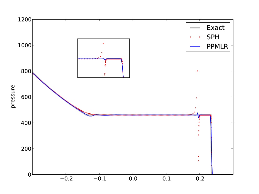
Figure 2: Numerical pressure for the blast-wave problem using SPH (dots), PPMLR (solid blue line) at $t=0.01s$ compared with the exact solution (solid black line). The pressure blip is visible for both SPH and PPMLR (see inset) schemes.

Numerical pressure profiles for the SPH and PPMLR schemes are shown in Fig. 2. We notice that the blip which was absent in the PPMLR solution for the Sod’s shock-tube problem is now present. Another striking feature is the huge jump in the pressure for the SPH solution. The results were generated using a total of $500$ particles for SPH and $500$ grid cells for PPMLR. At the outset, it may seem that the SPH results are no-where in comparison to PPMLR but this is not the case. This is because the PPMLR scheme has an inherent diffusion for the thermal energy which works to dissipate the error with time. Recall that we explicitly switched off the thermal conduction for the SPH scheme. With a small amount of thermal conduction, the results of the two schemes are similar as

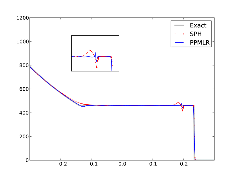
Figure 3: Numerical pressure for Blast-wave problem using SPH with thermal conduction (dots), PPMLR (solid blue line) at $t=0.01s$ compared with the exact solution (black line). The pressure blip produced by each of the schemes is now similar.

can be seen in Fig. 3, where the magnitude of the SPH pressure jump is dramatically reduced and is only slightly larger than that of the PPMLR scheme. Having established the presence of the numerical error for both schemes, we now proceed to a discussion on the nature of the error and provide an explanation for it’s occurrence.

3 A discussion on the error

In the previous section, we provided numerical evidence to support our original claim that the ubiquitous pressure jump at the contact discontinuity for SPH solutions, occurs for a class of finite difference schemes. In particular, the Lagrange plus remap version of the Piecewise Parabolic Method (PMPLR) results in an error remarkably similar to SPH. We note that although code comparisons for SPH and PPM in different contexts have previously been conducted ([2, 46, 4, 6]), this error has rather strangely gone unnoticed or has not been reported. It is possible that the comparisons were carried out with the fully Eulerian version of PPM, as two step (Lagrange plus remap) codes have traditionally fallen out in favour of their fully Eulerian counterparts. Indeed, Woodward and Colella [47], in their comparison of numerical schemes for flows with strong shocks showed that the cell-centred, direct Eulerian version of the PPM scheme (PPMDE) was the most accurate. In a more recent study, Pember and Anderson [48] argue otherwise, stating that the two approaches yield generally equivalent results. Nevertheless, direct Eulerian schemes are undoubtedly more prevalent and higher order versions of these schemes do not exhibit the SPH-like pressure jump at the contact, as can be verified by any of the schemes presented in the monographs by Toro [41] and LeVeque [42]. We believe the differences between the remap and direct Eulerian finite difference schemes could provide insight into the nature of the pressure jump in SPH. We would like to remind the reader that although we know of a suitable “fix” in the form of thermal conduction, we are looking for a consistent explanation for it’s origin and a justification for the myriad approaches outlined in the introduction.

3.1 The nature of the error

A natural question to ask of a numerical scheme is convergence to the physically correct solution. The pressure jump at the contact, being clearly erroneous, raises valid questions as to the behaviour of the error with the spatial resolution. It is instructive therefore, to catalogue known features of the pressure jump in the SPH context. We continue with the strong shock problem of Sec. 2.2 as the canonical example exposing this behaviour for SPH. Thermal conduction is switched off to avoid cosmetic smoothing of the results. Concerning the question of numerical convergence, we first examine the error as we increase the number of particles.

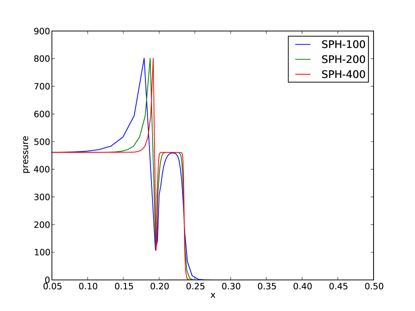
Figure 4: Numerical pressure for Blastwave problem using SPH with different resolutions. The solution profiles are expectedly more crisp for higher resolutions. The spread of the error reduces with increasing resolution but peak magnitude of the error remains constant.

Fig. 4 shows the results for the blastwave problem when we have used $100$, $200$ and $400$ particles respectively. The shock transition region is sharper with higher resolution as expected. We notice that the spread of the error reduces with increasing resolution but the peak point-wise error remains constant. Convergence in $L_{\infty}$ is therefore not possible in SPH. Convergence in $L_{1}$ with a convergence rate or approximately $2$ has been observed previously [37]. The temporal behaviour of the error can be studied through Fig. 5, which shows snapshots of the pressure profile at the times $t=0.0025$, $t=0.005$, $t=0.0075$ and $t=0.01$. These results highlight another feature of the error.

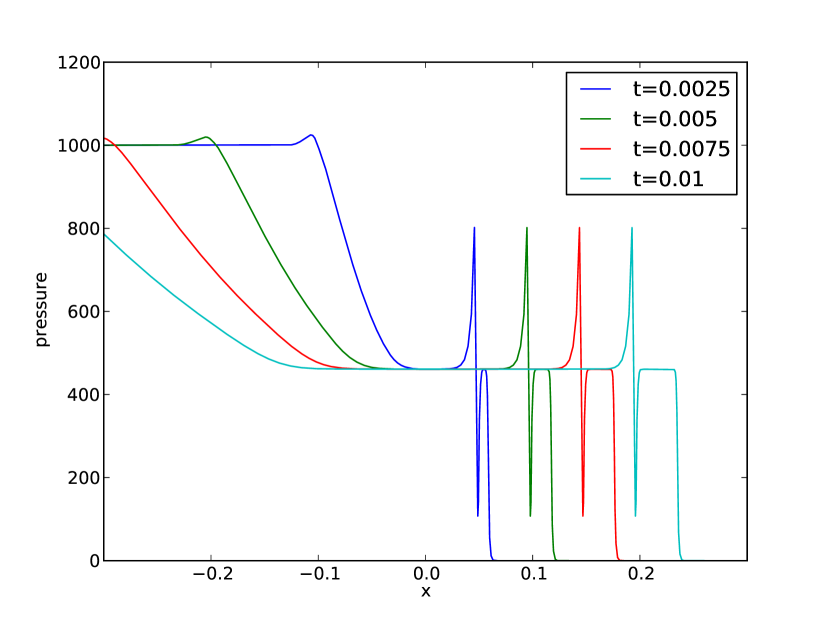
Figure 5: Numerical pressure for Blastwave problem at the time instants $t=0.0025$, $t=0.005$, $t=0.0075$ and $t=0.01$ seconds, when simulated with SPH. Once the pressure “blip” is generated, it is advected without dissipation. Thermal conduction was explicitly turned off to highlight this behaviour.

Namely, once the error is created, the pressure jump simply advects with the flow and neither grows nor attenuates without explicit thermal conduction. Artificial viscosity has no discernible effect on the solution. This is not surprising when we consider that the artificial viscosity is added to generate the correct entropy jump across the shock and therefore, has no effect at the contact discontinuity. To summarize, the pressure jump at the contact discontinuity, in the context of SPH has the following properties:

• The error, once created is simply advected with the material velocity.

• With the increase of spatial resolution, the spread of the error decreases whilst maintaining a constant peak magnitude.

• Artificial viscosity has no role to play in suppressing or mitigating it’s effect.

3.2 The relation to wall-heating errors

A multi-valued pressure in the presence of an accurate density profile results, in a corresponding jump in the thermal energy, via the equation of state. The pressure jump in SPH can therefore be thought of as a spurious heating/cooling of the fluid. For the numerical solution of the compressible Euler equations, “wall-heating” is the canonical term given to errors that result in a spurious rise in thermal energy (heating). The problem has generated considerable interest and has received the attention of several researchers [49]. The term was coined by Noh. [50] when he considered the problem of shock reflection in planar, cylindrical and spherical geometries. The reason for our interest in these errors is the similarity it bears with the SPH errors at the contact discontinuity. For instance, under mesh refinement, Noh observed that the overheating decreases in spatial range while maintaining it’s peak point-wise value. This leads Noh to conjecture that the error is built into the exact solution of the modified viscous equations. He further argues that any numerical method based on “shock-smearing” (artificial viscosity) will demonstrate this error. By considering the asymptotic solution of the governing equations with artificial viscosity, Menikoff [51] argues that entropy errors, resulting in spurious heating/cooling are generated not only for shock reflection, but also for shock interaction or when a shock passes through a change in mesh spacing. The errors are generated over a short transient phase as a result of the numerical width of the shock. After the initial transient phase, the entropy errors are frozen and simply advected with the fluid and the only recourse is to add thermal conduction which leads to a diffusion of the energy. A similar analysis in Lagrangian coordinates was carried out by Shen et al. [43]. Once again, entropy errors were observed to occur over a short, initial transient phase of shock interaction/reflection.
These observations for wall heating errors in the context of traditional finite volume methods bear a striking similarity to the SPH pressure/entropy errors. Thus, we conjecture that the SPH errors are a form of spurious heating that occurs in an initial transient phase. Once the entropy errors are generated, diffusion of entropy (thermal conduction) is the only recourse to mitigate it’s effect.

4 An Explanation for the Error

We argued that the pressure jump at the contact discontinuity for SPH has symptoms of wall-heating errors previously observed for traditional finite difference/volume codes. Essentially, an entropy error is generated during the initial transient phase of shock formation, the magnitude of which is independent of the spatial resolution. After the initial transient, the error is convected along the particle trajectories without dissipation. Monaghan and Gingold. [1] had originally ascribed this anomalous behaviour for SPH, to generic “starting” errors. More than twenty years later, Tasker et al. [6] had also suggested that the discontinuous initial conditions give rise to an entropy error. Since the errors are generated at start-up, and subsequently passively advected with the particles, thermal conduction is required to mitigate it’s effect. This was the also the conclusion drawn by Noh. [50] when he proposed an artificial heat flux for finite difference schemes. While this reasoning serves to justify the artificial conductivity approach in treating the error, it sheds no light onto the origins of the error. Towards this aim, we adopt a different perspective by studying grid-based schemes.
Recall that in Sec. 2, the errors for the Lagrange plus Eulerian remap version of the PPM scheme (PPMLR) was shown to be qualitatively similar to those of SPH. Agreeing with the reasoning of Davies et al. [2], we find it highly unlikely that two fundamentally different schemes (SPH and PPMLR) would result in the same erroneous features. This leads us to believe that both schemes solve a similar modified equation, the solution of which exhibits the heating and corresponding pressure jump at the contact. A scaling argument similar to Noh. [50] shows that the magnitude of the error is independent of the spatial resolution. This justifies to some extent the claim that the error is built into the exact solution of the discrete SPH equations. It is therefore reasonable to assume that a solution to the problem within the finite volume context using PPMLR might provide clues for a similar resolution in SPH. This can be done by comparing the Lagrangian plus remap PPM scheme, PPMLR, with it’s direct Eulerian counterpart, PPMDE, for which the error is absent.

4.1 PPMLR and PPMDE

The Piecewise Parabolic Method (PPM) [38] is a high order, Godunov finite difference method that has, as it’s building block, a third order advection scheme. Along with the ENO/WENO type schemes [52], PPM is considered to be a highly accurate method for the compressible Euler equations [47]. The scheme, as originally proposed by Colella and Woodward [38], can be formulated to follow either Lagrangian or Eulerian hydrodynamics. Although the two equation sets are mathematically the same, their numerical solutions exhibit differences which we are interested in.
In what follows, we focus on the development of the one-dimensional PPM scheme since multi-dimensional extensions are constructed with the dimensional splitting approach. Thus, essential details of the method and the error producing mechanism in particular are contained within the one-dimensional scheme. In a such a scheme, the conserved variables are the specific volume $1/\rho$, velocity $u$, and the specific energy $\hat{e}=e+\frac{1}{2}u^{2}$ for the Lagrangian formulation, and density $\rho$, momentum $\rho u$, and total energy $\rho\hat{e}$, for the Eulerian formulation. Both versions of the PPM scheme (PPMLR, PPMDE) advance the solution (vector of conserved variables $\boldsymbol{U}$) over physical zones or cells. The generic $i^{\text{th}}$ cell has it’s center at $x_{i}$, left and right faces at $x_{i-\frac{1}{2}}$ and $x_{i+\frac{1}{2}}$ respectively and $\Delta x_{i}=x_{i+\frac{1}{2}}-x_{i-\frac{1}{2}}$ denotes the cell volume.

4.1.1 PPMLR

The conservative equations for Lagrangian hydrodynamics are given as

$$\tau_{t}-u_{\xi} =0$$ (1a)

$$u_{t}+p_{\xi} =0$$ (1b)

$$\hat{e}_{t}+(pu)_{\xi} =0$$ (1c)

where $\tau=1/\rho$ is the specific volume, $\hat{e}=\frac{1}{2}u^{2}+e$ is the total energy per unit mass and the time derivative is to be understood as a derivative moving with the fluid (material derivative) $\frac{d}{dt}(*)=\frac{\partial}{\partial t}(*)+u\nabla(*)$. $\xi$ is the mass coordinate, which is related to the spatial coordinate $x$, through the transformation $d\xi=\rho dx$. The system is hyperbolic with eigenvalues $\lambda_{1}=-C$, $\lambda_{2}=0$ and $\lambda_{3}=C$, where $C=(\gamma p\rho)^{\frac{1}{2}}$ is the Lagrangian sound speed. The convective terms are absent in this formulation which is reflected as a wave of speed $0$.
In PPMLR, the procedure to advance the solution is carried out in two steps. In the first step, piecewise parabolic interpolations of the pressure, velocity and density are used to compute the effective left and right states for a Riemann problem between two adjacent cells. Since the zone edge is moving with the fluid velocity, the input state is determined purely by the acoustic modes $\lambda_{1}$ and $\lambda_{3}$. With the input (left, right) states constructed from the parabolic reconstructions, a Riemann problem is solved to calculate fluxes through the cell boundaries. The vector of conserved variables are updated using the conservative differencing equations:

$$x_{j+\frac{1}{2}}^{n+1} =x_{j+\frac{1}{2}}^{n}+\Delta t\overline{u}_{j+\frac{1}{2}}$$ (2a)

$$\tau_{j+\frac{1}{2}}^{n+1} =\frac{1}{\Delta m_{j}}\left(x_{j+\frac{1}{2}}^{n+1}-x_{j-\frac{1}{2}}^{n+1}\right)$$ (2b)

$$u_{j+\frac{1}{2}}^{n+1} =u_{j+\frac{1}{2}}^{n}+\frac{\Delta t}{\Delta m_{j}}\left(\overline{p}_{j-\frac{1}{2}}-\overline{p}_{j+\frac{1}{2}}\right)$$ (2c)

$$\hat{e}_{j+\frac{1}{2}}^{n+1} =u_{j+\frac{1}{2}}^{n}+\frac{\Delta t}{\Delta m_{j}}\left(\overline{u}_{j-\frac{1}{2}}\overline{p}_{j-\frac{1}{2}}-\overline{u}_{j+\frac{1}{2}}\overline{p}_{j+\frac{1}{2}}\right)$$ (2d)

In these equations, $\overline{p}$ and $\overline{u}$ denote the intermediate pressure and velocity that results from the solution to Riemann problem at a zone edge. Convection is introduced through the cell motion. After the advection step, the solution is conservatively re-mapped onto the original Eulerian grid. A necessary condition for high-order Godunov schemes, non-linearity is introduced by using limiters and monotonicity constraints in the piecewise parabolic data reconstruction.

4.1.2 PPMDE

The one-dimensional equations for Eulerian, inviscid hydrodynamics are given as

$$\rho_{t}+(\rho u)_{x} =0$$ (3a)

$$(\rho u)_{t}+(\rho u^{2}+p)_{x} =0$$ (3b)

$$(\rho\hat{e})_{t}+(\rho\hat{e}u+pu)_{x} =0$$ (3c)

where the symbols have the same meaning and $(*)_{t}$ is the partial derivative with respect to time. The system of equations is again hyperbolic with eigenvalues $\lambda_{1}=u-c$, $\lambda_{2}=u$ and $\lambda_{3}=u+c$, where $c=\rho C$, is the Eulerian sound speed. The procedure to update the solution in the one-step, direct Eulerian formulation is essentially the same as PPMLR. Piecewise parabolic interpolations of the dependent variables are used to compute effective left and right states for Riemann problems between adjacent cells. Zone fluxes, computed from the Riemann solution are used in a conservative differencing scheme.

$$\boldsymbol{U}_{j+\frac{1}{2}}^{n+1} =\boldsymbol{U}_{j+\frac{1}{2}}^{n}+\frac{\Delta t}{\Delta x_{j}}\left(\boldsymbol{F}(\overline{\boldsymbol{U}}_{j-\frac{1}{2}})-\boldsymbol{F}(\overline{\boldsymbol{U}}_{j+\frac{1}{2}})\right)$$ (4a)

$$\overline{\boldsymbol{U}}_{j+\frac{1}{2}} \approx\frac{1}{\Delta t}\int_{t^{n}}^{t^{n+1}}\boldsymbol{U}(x_{j+\frac{1}{2}},t)dt$$ (4b)

The difference is in the construction of the input states for the Riemann problem. This is now more complicated than the Lagrangian case as there may now be as many as $3$ and as few as $0$ waves impinging on a zone edge from a given side. A consequence of this is that in general, for the input state at a given zone edge, contributions from each wave family must be accounted for [38].

4.2 Diffusion in the material wave

Both PPMLR and PPMDE employ piecewise parabolic interpolations of the cell centered density, pressure and velocity to construct the input left and right states as integral averages over the characteristic domain of dependence. The domain of dependence for a given wave family is defined by tracing back the path of the wave if it impinges on the zone edge from a given side. For the Lagrangian formulation, we have two waves corresponding to the acoustic modes, $\lambda_{1}$ and $\lambda_{3}$. The material wave is absent as the cells are assumed to move with the local fluid velocity ($\lambda_{2}=0$). For the Eulerian formulation, waves from each of the three families can impinge on an edge from a given side. The input state in this case is constructed such that the amount of wave associated with each family of characteristics transported across a zone edge is correct up to terms of second order [38]. Thus, the additional material wave must be accounted for in the Eulerian formulation. Diffusion across this wave is the main difference between the two versions of PPM. Indeed, Eulerian Godunov schemes are known to be more diffusive at the contact when compared to Lagrangian formulations. This was highlighted by Woodward and Colella [47] and later by Pember and Anderson [48], when they compared remap and direct Eulerian finite volume schemes.

Figure 6: Results for the blast-wave problem using a remap code with piecewise parabolic (PPMLR) and piecewise constant (PCMLR) interpolations. The entropy error (pressure jump) is eliminated with when using the diffusive PCMLR method.

This suggests a lack of dissipation is actually the cause of the SPH-like entropy error for PPMLR as observed in Sec. 2. It was suggested by Jim Stone (private communication, August 2013) that the low dissipation in PPM causes these “start-up” errors. The discontinuous initial conditions gives rise to additional waves on a discrete level which is captured by the low dissipative schemes like PPMLR. One is then tempted to verify the hypothesis by constructing a more diffusive version of the PPMLR scheme. The easiest way to do this is to use a piecewise constant reconstruction instead of the parabolic reconstruction used in PPMLR. Results for the blast-wave problem using such a scheme (PCMLR) is shown in Fig. 6. The solution is expectedly less crisp than PPMLR but remarkably, the pressure jump at the contact is eliminated. We note that it is not possible for the remap phase of PPMLR to introduce the error. This is because remapping can be viewed as a projection and is inherently a diffusive process. As a result, no new extrema can occur in this step. The error is therefore generated in the Lagrangian advection phase.
What does dissipation in the material wave look like? To answer this question, we consider the eigenstructure of the equations in the Lagrangian formulation (Eq. 1). The right and left eigenvectors for this hyperbolic system is given as ([53])

$$R=\begin{pmatrix}1&1&1\\ C&0&-C\\ uC-p&\frac{p}{\gamma-1}&-uC-p\end{pmatrix},\,\,\,R^{-1}=\begin{pmatrix}\frac{1}{2\gamma}&\frac{1}{2C}+\frac{u(\gamma-1)}{2\gamma p}&\frac{1-\gamma}{2\gamma p}\\ \frac{\gamma-1}{\gamma}&\frac{u(\gamma-1)}{\gamma p}&\frac{\gamma-1}{\gamma p}\\ \frac{1}{2\gamma}&-\frac{1}{2C}+\frac{u(\gamma-1)}{2\gamma p}&\frac{1-\gamma}{2\gamma p}\end{pmatrix}$$ (5)

where $C=(\gamma p\rho)^{\frac{1}{2}}$ is the Lagrangian sound speed. A conservative finite volume scheme with a general diffusive flux contribution can be defined as

$$\left(\boldsymbol{F}_{j+\frac{1}{2}}\right)_{\text{diss}}=-\frac{1}{2}\sum_{k=1}^{3}\hat{\boldsymbol{r}}_{k}|\hat{\lambda}_{k}|\left(\hat{\boldsymbol{r}}_{k}^{-1}\cdot\Delta\hat{\boldsymbol{U}}_{j+\frac{1}{2}}\right),$$ (6)

where the caret denotes a suitably averaged value at the zone interface $x_{j+\frac{1}{2}}$. This is the numerical flux for linearized schemes such as Roe’s scheme [54] and is applicable to SPH [15, 34]. The diffusive flux in Eq. 6 computes jumps across each wave family. The magnitude of the jump (wave strength), $\alpha=\hat{\boldsymbol{r}}_{k}^{-1}\cdot\Delta\hat{\boldsymbol{U}}$, is weighted by the wave speed. The final contribution to the conserved variables is determined by the right eigenvector for that wave family. For the Lagrangian scheme, this contribution vanishes for the material wave ($k=2$), since $\lambda_{2}=0$. This is the contribution we are interested in, the algebraic form of which is given by

$$\left(f_{j+\frac{1}{2}}^{2}\right)_{\text{diss}}=-|\lambda_{2}|\frac{1}{2}\,\begin{bmatrix}\frac{1}{2C}+\frac{u(\gamma-1)}{2\gamma p}&\frac{u(1-\gamma)}{\gamma p}&-\frac{1}{2C}+\frac{u(\gamma-1)}{2\gamma p}\end{bmatrix}\cdot\begin{bmatrix}\Delta\hat{\tau}\\ \Delta\hat{u}\\ \Delta\hat{e}\end{bmatrix}\begin{bmatrix}1\\ 0\\ \frac{p}{\gamma-1}\end{bmatrix}$$ (7)

Due to the structure of the right eigenvector ($\boldsymbol{r}_{2}$ in Eq. 5), the dissipation acts on the first and third components of $\boldsymbol{U}$. For the Lagrangian formulation, these are the specific volume $\tau=1/\rho$, and total energy per uni mass $\hat{e}=\frac{1}{2}u^{2}+e$ respectively. Thus, dissipation in the material wave would result in an additional density and energy diffusion simultaneously that is absent in a purely Lagrangian formulation.

5 Application to SPH

The lack of dissipation in the material wave, coupled with the low diffusion of PPMLR is responsible for the entropy errors, and hence the SPH-like pressure jump at the contact. The introduction of dissipation helped eliminate the error for the finite volume remap code in Sec. 4. It is then reasonable to assume that an improvement of results can be expected for SPH if this dissipation is somehow introduced. Indeed, this has been the adopted practice within the SPH community, with dissipation often introduced directly through thermal conduction [11, 14, 16, 17, 22, 18, 25], or via surrogate means such as using a smoother estimate to define particle volume [27, 28], relaxing initial conditions [18, 19] and a modification to the equation of state [33]. The problem with the dissipation introduced in these schemes is that they appear serendipitous and their reasoning belies the simplicity of the SPH formulation. The requirement that dissipation should act across the material wave provides a consistent explanation as to why the aforementioned approaches work. From Eq. 7, we know that a combination of dissipation in the density and energy variables is required to suppress the entropy errors. Dissipation for velocity (artificial viscosity) has no role to play. This was verified numerically in Sec. 3. Armed with this knowledge, we can attempt to introduce the requisite dissipation in a consistent manner for SPH, thereby validating our hypothesis.

5.1 Adding diffusion to SPH

We consider the GSPH formulation [30] with an approximate Riemann solver. We have shown ([34]) that with a suitable choice of an approximate Riemann solver, this formulation is equivalent to a variational SPH scheme with artificial dissipation and thermal conduction. The advantage of this formulation is the explicit control of the dissipation through numerical fluxes akin to finite difference/volume schemes. The discrete SPH equations in this formulation, for the density, velocity and thermal energy are given as

$$\rho_{a} =\sum_{b\in\mathcal{N}(a)}m_{b}W_{ab}(h_{a})$$ (8a)

$$\ddot{\boldsymbol{x}}_{a} =-\sum_{b\in\mathcal{N}(a)}m_{b}p^{*}_{ab}\left(\frac{1}{\rho_{a}^{2}}\nabla W_{ab}(h_{a})+\frac{1}{\rho_{b}^{2}}\nabla W_{ab}(h_{b})\right)$$ (8b)

$$\dot{e}_{a} =-\sum_{b\in\mathcal{N}(a)}m_{b}p^{*}_{ab}[\boldsymbol{v}_{ab}^{*}-\dot{\boldsymbol{x}}_{a}]\left(\frac{1}{\rho_{a}^{2}}\nabla W_{ab}(h_{a})+\frac{1}{\rho_{b}^{2}}\nabla W_{ab}(h_{b})\right)$$ (8c)

where, the starred quantities ($p^{*},\,\boldsymbol{v}^{*}$) are the intermediate state arising from the solution of a Riemann problem between two interacting particles. The solution to the Riemann problem introduces the minimum and necessary dissipation required to stabilize the scheme.
We follow the approach proposed by Shen et al. [43] by constructing a hybrid scheme in which a regular Riemann solver is used in the momentum equation equation, and a diffusive Riemann solver is used for the energy equation. Recall that the flux vector for the conservative equations in the Lagrangian formulation are $\left(-u,p,pu\right)$. Thus, using a more dissipative intermediate velocity is akin to introducing dissipation in the density and energy equations. In [34], we evaluated $5$ different approximate Riemann solvers in Lagrangian coordinates for use with GSPH. From an analysis of an accuracy test for the Euler equations, we find that the Harten, Lax, van Leer and Einfeldt (HLLE) [53] solver is a suitable choice for the diffusive approximate Riemann solver. For the regular Riemann solver, we can use any one from the exact [55], Ducowicz [56] or Roe [54] approximate Riemann solvers.

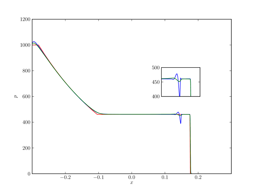
Figure 7: Numerical pressure profiles for the blastwave problem using standard GSPH (blue) and the hybrid GSPH (green) using the HLLE approximate Riemann solver, compared with the exact solution (ref). The HLLE solver is successful in suppressing the entropy errors as can be seen in the inset plot.

We construct such a scheme, where the two approximate Riemann solvers used are the van Leer exact and the HLLE approximate Riemann solver. In particular, the diffusive contribution is constructed as

$$u^{*} =\frac{1}{t_{f}}(tu^{*}_{\text{regular}}+(t_{f}-t)u^{*}_{\text{diff}}),$$ (9a)

$$p^{*} =\frac{1}{t_{f}}(tp^{*}_{\text{regular}}+(t_{f}-t)p^{*}_{\text{diff}}),$$ (9b)

where, $t_{f}$ is the final time in the simulation. This corresponds to a linear blending of the two estimates with a more diffusive estimate used in the initial stages of the computation. Since the errors are expected to be generated at start-up, the blending avoids excessive dissipation that may ruin the solution. Fig. 7 shows the numerical pressure profiles for the standard (blue) and hybrid GSPH (green), compared with the exact solution (red), when using $1000$ equal mass particles. As expected, the dissipation helps to suppress the entropy error, with only a slight kink visible in the inset plot.

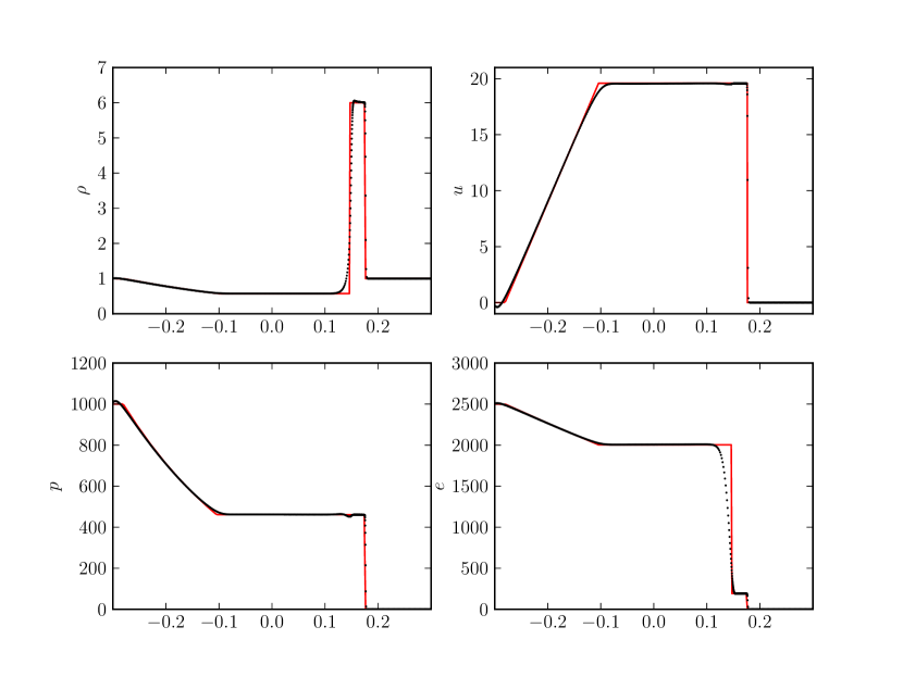
Figure 8: Numerical solution (dots) for the hybrid GSPH compared with the exact solution (red). The hybrid scheme shows good agreement with the exact solution with a negligible pressure jump. The dissipation has the desired effect of acting on the contact discontinuity.

The suppression of the pressure jump at the contact discontinuity does not have an adverse effect on the profiles of the other physical variables as can be seen in Fig. 8, which shows the numerical solution for the hybrid GSPH scheme (dots), compared with the exact solution (red line). The dissipation has the desired effect of acting on the contact discontinuity as can be observed by the slightly smeared density and thermal energy profiles. near $x\approx 0.15$.

We would like to point out that this method produces improved results than with using a traditional scheme with larger thermal conduction parameters. Fig. 9 shows the result of simply increasing the thermal conduction parameter $\alpha_{u}$, for the variational scheme of Monaghan, Price and Morris [15, 57, 26].

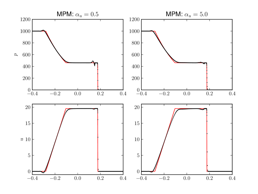
Figure 9: Effect of increasing the thermal conduction parameter $\alpha_{u}$ for the MPM scheme. Larger values of the parameter (right) mitigate the jump in the pressure (upper panel) but also generates a corresponding dip in the velocity profile (lower panel).

Larger values of the thermal conduction parameter works to supress the presure discontinuity as expected. However, results in an unwanted dip in the velocity profile at the contact discontinuity. This behaviour has been recently reported by Sirotkin and Yoh [58] in their SPH scheme with approximate Riemann solvers. In comparison, the hybrid GSPH scheme (cf Fig. 8) does not produce this behaviour.

5.2 Consequences of adding dissipation

The linear blending of the two estimates for $\boldsymbol{v}^{*}$ through Eq. 9 was shown to work well to suppress the pressure jump for the one-dimensional blast-wave problem. Since the errors are expected to be generated at start-up, it’s use can be detrimental for long time simulations.

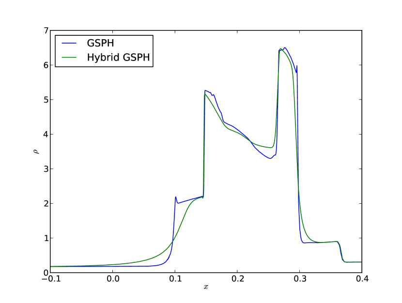
Figure 10: Density profiles at $t=0.038$ for the Woodward and Colella blast-wave problem using standard GSPH (blue) and the hybrid modification (green) using Eq. 9. The contact discontinuities near $x=0.1$ and $x=0.3$ are heavily smeared for the hybrid scheme and the solution within $x\in[0.15,0.3]$ has lost some detail.

For example, Fig. 10 shows the density profiles for the Woodward and Colella blast-wave problem [47, 45] using standard GSPH (blue) and the hybrid modification (green) at the time $t=0.038$. The extra dissipation in the hybrid scheme has resulted in an excessive smearing of the contact discontinuities near $x=0.1$ and $x=0.3$, and a loss of detail within the region $x\in[0.15,0.3]$. Note that adding dissipation to the material wave (contact discontinuity) is exactly what we set out to do, although Eq. 9 results in an over diffusive scheme. This can be corrected by defining the intermediate states as

$$u^{*} =u^{*}_{\text{regular}}+e^{-\alpha\frac{t}{t_{f}}}\left(u^{*}_{\text{diff}}-u^{*}_{\text{regular}}\right)$$ (10a)

$$p^{*} =p^{*}_{\text{regular}}+e^{-\alpha\frac{t}{t_{f}}}\left(p^{*}_{\text{diff}}-p^{*}_{\text{regular}}\right)$$ (10b)

This corresponds to an exponential decay with time, for the diffusive component. The parameter $\alpha$, controls the rate of decay (growth) of the two velocity estimates, with higher values resulting in a more rapid decay (growth).

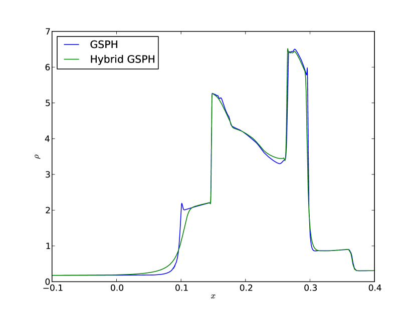
Figure 11: Density profiles at $t=0.038$ for the Woodward and Colella blast-wave problem using standard GSPH (blue) and the hybrid modification (green) using Eq. 10 and $\alpha=10$. The solution is expectedly more crisp with a good agreement in the region $x\in[0.15,0.3]$

Fig. 11 shows the density profiles at $t=0.038$ for the same problem when we have this blending function with $\alpha=10$. The density profile for the hybrid GSPH (green) scheme is expectedly more crisp with an improved agreement with the second order GSPH (blue) scheme in the region $x\in[-0.15,0.3]$.

Fig. 11 shows the density profiles at $t=0.038$ for the same problem when we have this blending function with $\alpha=10$. The density profile for the hybrid GSPH (green) scheme is expectedly more crisp with an improved agreement with the second order GSPH (blue) scheme in the region $x\in[-0.15,0.3]$.
We concede that a tuning parameter to control dissipation perhaps goes against the ethos of a GSPH scheme that is inherently parameter free. While one can argue that the choice of the Riemann solver itself in the GSPH scheme can be thought of as a parameter, the issue we want to highlight is the subtle role of dissipation, that is needed for stability but criticized when used in excess. An ideal scheme should use just the right amount of dissipation for all problems, the requisite amount, in turn, ideally determined by the scheme itself (adaptive schemes). High-order Godunov methods (MUSCL, PPM, ENO/WENO) are generally accepted to fit this ideal. However, Quirk [59] famously pointed out several instances where these schemes fail or produce erroneous results. Moreover, he suggests that most of these errors can be overcome by a judicious use of artificial dissipation. The trick is to avoid a proliferation of tuning parameters to determine the requisite dissipation. We are faced with a similar conundrum while constructing our hybrid GSPH scheme. Dissipation must be somehow introduced into the purely inviscid equations and in this work we have argued in favour of a specific form, acting across the energy and density variables to suppress entropy errors. Given the transient nature of the error, we are forced to introduce a parameter that limits the extra dissipation to when it is needed.

5.3 Extension to higher dimensions

We used the one-dimensional blast-wave problem as the canonical test highlighting the SPH entropy errors. The manner in which we chose to introduce the dissipation is however, not limited to the one-dimensional case. This can bee seen in Fig. 12, which shows the numerical (dots) pressure for the hybrid scheme (green) compared with the reference second order GSPH scheme (blue) with the van Leer Riemann solver, for a two-dimensional blastwave problem.

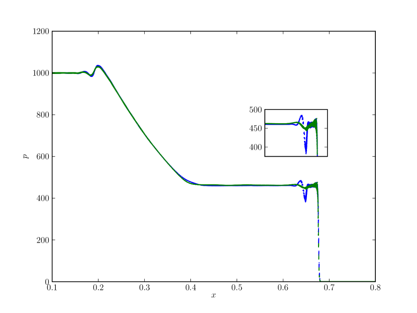
Figure 12: Numerical pressure for the hybrid GSPH (green) scheme with $\alpha=3.0$ and with the choice of HLLE as the diffusive Riemann solver, compared with the standard second order GSPH scheme using the van Leer exact Riemann solver (blue). The results are exactly analogous to the one-dimensional case (Fig. 7), with the hybrid scheme working well to limit the pressure jump.

For the hybrid scheme, we use the exponential smoothing given by Eqs. 10 with $\alpha=3.0$, and choose the HLLE solver as the diffusive Riemann solver. The suppression of the pressure blip has no discernible adverse effect on the other variables as can be seen in Fig. 13, which shows the density (left), velocity (center) and thermal energy (right) for the hybrid GSPH scheme (lower panel), compared with a second order GSPH scheme using the van Leer exact Riemann solver (upper panel).

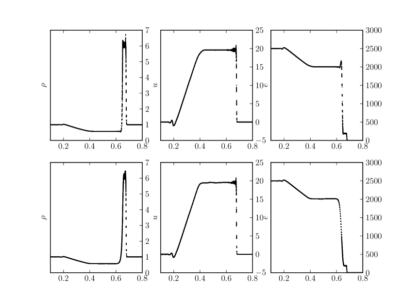
Figure 13: Numerical solution for the hybrid GSPH scheme (lower panel) with $\alpha=3$ and with the choice of HLLE as the diffusive Riemann solver, compared with the standard second order GSPH scheme (upper panel). The hybrid scheme works to suppress the pressure blip (Fig. 12) and has no discernible adverse effect on the other physical variables. In particular, the spike in the thermal energy behind the contact is eliminated. Additionally, the contact discontinuity is slightly smeared for the density.

The hybrid scheme eliminates the spike in the thermal energy behind the contact. Additionally, analogous to the one-dimensional case, the contact discontinuity is slightly smeared as can be seen in the density plot around $x\approx 0.6$. The results were generated using a total of $20000$ equal mass particles initially distributed in a hexagonal close paced arrangement.

6 Summary and further work

In this work, we attempted to provide an explanation for the origin of the ubiquitous pressure jump in SPH simulations of the compressible Euler equations. The anomalous behaviour has been observed since the dawn of SPH [1] and has received attention ever since. It has been highlighted as a drawback of the method when compared with traditional Eulerian schemes [4, 6], and has led some researchers to develop particle tessellation techniques as an alternative to SPH [60, 61]. Within the SPH community, the use of dissipation, introduced via various means has been the general recourse to mitigate the effects of the error.

Through an analogy with “wall heating” errors for finite difference/volume codes, we argued that the pressure jump is a result of entropy errors generated over an initial transient phase and thereafter, passively advected with the particles. We highlighted that a qualitatively similar error is present for the Lagrange plus remap version of the Piecewise Parabolic Method (PPM) finite volume code PPMLR. Through a comparison of PPMLR with it’s direct Eulerian counterpart, PPMDE, a lack of diffusion across the material wave was identified as the origin for the error. By examining the eigenstructure of the Lagrangian equations of motion, we showed that the requisite diffusion needs to act on the density and energy equations simultaneously. This explanation also justifies the myriad techniques employed by different researchers to “cure” the problem. Using our hypothesis, we construct a hybrid GSPH scheme that introduces the requisite dissipation by using a more diffusive flux for the energy equation. We verified our hypothesis by using the blast-wave problem as the canonical test highlighting the pressure anomaly in SPH. The results using the new scheme are shown to be better than simply increasing the magnitude of thermal conduction for SPH schemes that rely on explicit dissipation. A tuning parameter is introduced to limit the dissipation to the initial stages of the computation.

We expect the added dissipation to be disadvantageous for certain problems. An example is the Sjögreen’s strong rarefaction test (1-2-3 problem [41]), for which, numerical dissipation should be kept to a minimum. Indeed, one of the advantages of the SPH artificial viscosity is the ability to switch it off entirely when not required. Additionally, we believe that the hybrid GSPH scheme can certainly be improved upon by using an alternative hybridization to Eqs. 10. These equations were constructed for the specific example to validate our hypothesis concerning the origin of the spurious pressure jump in SPH. The construction of an adaptive hybridization and validation for a general suite of multi-dimensional problems is left as an area for future investigation.

References

- Monaghan and Gingold [1983] Monaghan, J., Gingold, R.. Shock Simulation by the Particle Method SPH. Journal of Computational Physics 1983;52:374–389.
- M.B. Davies and M. Ruffert and W. Benz and E. Müller [1993] M.B. Davies and M. Ruffert and W. Benz and E. Müller, . A comparison between SPH and PPM: simulations of stellar collisions. Astronomy and Astrophysics 1993;272:430–411.
- M. Steinmetz and E. Müller [1993] M. Steinmetz and E. Müller, . On the capabilities and limits of smooth particle hydrodynamics. Astronomy and Astrophysics 1993;268:391–410.
- Agertz et al. [2007] Agertz et al., . Fundamental differences between SPH and grid methods. Monthly Notices of the Royal Astronomical Scociety 2007;380:963–978.
- Volker Springel [2005] Volker Springel, . The cosmological simulation code GADGET-2. Monthly Notices of the Royal Astronomical Scociety 2005;364:1105–1134.
- Tasker et al. [2008] Tasker et al., . A test suite for quantitative comparison of hydrodynamic codes in astrophysics. Monthly Notices of the Royal Astronomical Scociety 2008;390:1267–1281.
- Takashi Okamoto and Adrian Jenkins and Vincent R. Eke and Vincent Quils [2003] Takashi Okamoto and Adrian Jenkins and Vincent R. Eke and Vincent Quils, . Momentum transfer across shear flows in smoothed particle hydrodynamics simulations of galaxy formation. Monthly Notices of the Royal Astronomical Scociety 2003;345:429–446.
- M. Herant [1994] M. Herant, . Dirty Tricks for SPH (Invited paper). Memorie della Societa Astronomica Italiana 1994;65:1013–1022.
- Monaghan [1992] Monaghan, J.. Smoothed Particle Hydrodynamics. Annual Review of Astronomy and Astrophysics 1992;30:543–574.
- Leigh Brookshaw [1994] Leigh Brookshaw, . Solving the Heat Diffusion Equation in SPH. Memorie della Scociet‘a Astronomia Italiana 1994;65:1033–1042.
- Sigalotti et al. [2006] Sigalotti, L.D.G., Lopex, H., Donoso, A., Siraa, E., Klapp, J.. A shock capturing sph scheme based on adaptive kernel estimation. Journal of Computational Physics 2006;212:124–149.
- Sigalotti et al. [2008] Sigalotti, L.D.G., Lopex, H., Trujillo, L.. An adaptive sph method for strong shocks. Journal of Computational Physics 2008;228:5588–5907.
- Stephan Rosswog and Daniel Price [2007] Stephan Rosswog and Daniel Price, . MAGMA: a three dimensional, Lagrangian magnetohydrodynamics code for merger applications. Monthly Notices of the Royal Astronomical Scociety 2007;379:915–931.
- Price [2008] Price, D.. Modelling Discontinuities and Kelvin-Helmholtz instabilities in SPH. Journal of Computational Physics 2008;227:10040–10057.
- Monaghan [1997] Monaghan, J.. SPH and Riemann Solvers. Journal of Computational Physics 1997;136:298–307.
- Wadsley et al. [2008] Wadsley, J.W., Veeravalli, G., Couchman, H.M.P.. On the treatment of entropy mixing in numerical cosmology. Monthly Notices of the Royal Astronomical Society 2008;387(1):427–438.
- García-Senz et al. [2009] García-Senz, D., Relan̈o, A., Cabez’on, R.M., Bravo, E.. Axisymmetric smoothed particle hydrodynamics with self-gravity. Monthly Notices of the Royal Astronomical Society 2009;392(1):346–360.
- S. Valcke and S. De Rijcke and E. Rödiger and H. Dejonghe [2010] S. Valcke and S. De Rijcke and E. Rödiger and H. Dejonghe, . Kelvin-Helmholtz instabilities in smoothed particle hydrodynamics. Monthly Notices of the Royal Astronomical Scociety 2010;408:71–86.
- J. I. Read and T. Hayfield and O. Agertz [2010] J. I. Read and T. Hayfield and O. Agertz, . Resolving mixing in smoothed particle hydrodynamics. Monthly Notices of the Royal Astronomical Scociety 2010;405:1513–1530.
- R. Valdarnini [2012] R. Valdarnini, . Hydrodynamic capabilities of an SPH code incorporating an artificial conductivity term with a gravity-based signal velocity. Astronomy and Astrophysics 2012;546:25.
- D. Kawata and T. Okamoto and B.K. Gibson and D.J. Barnes and R. Cen [2013] D. Kawata and T. Okamoto and B.K. Gibson and D.J. Barnes and R. Cen, . Calibrating an updated smoothed particle hydrodynamics scheme within GCD+. Monthly Notices of the Royal Astronomical Scociety 2013;428:1968–1979.
- Stephan Rosswog [2009] Stephan Rosswog, . Astrophysical smooth particle hydrodynamis. New Astronomy Reviews 2009;53:78–104.
- Ritchie and Thomas [2001] Ritchie, B.W., Thomas, P.A.. Multiphase smoothed-particle hydrodynamics. Monthly Notices of the Royal Astronomical Society 2001;323(3):743–756.
- Marri and White [2003] Marri, S., White, S.D.M.. Smoothed particle hydrodynamics for galaxy-formation simulations: improved treatments of multiphase gas, of star formation and of supernovae feedback. Monthly Notices of the Royal Astronomical Society 2003;345(2):561–574.
- J. I. Read and T. Hayfield [2012] J. I. Read and T. Hayfield, . SPHS: smoothed particle hydrodynamics with a high order dissipation switch. Monthly Notices of the Royal Astronomical Scociety 2012;422:3037–3055.
- Price [2012] Price, D.. Smoothed particle hydrodynamics and magnetohydrodynamics. Journal of Computational Physics 2012;231:759–794.
- Takayuki R. Saitoh and Junichiro Makino [2013] Takayuki R. Saitoh and Junichiro Makino, . A Density Independent Formulation of Smoothed Particle Hydrodyamics. 2013.
- Philip F. Hopkins [2002] Philip F. Hopkins, . A General Class of Lagrangian Smoothed Particle Hydrodyamics Methods and Implications for Fluid Mixing Problems. Monthly Notices of the Royal Astronomical Scociety 2002;333:649–664.
- Hu et al. [2014] Hu, C.Y., Naab, T., Walch, S., Mooster, B.P., Oser, L.. SPHGal: Smoothed Particle Hydrodynamics with improved accuracy for Galaxy simulations; 2014. zrXiv:1402.1788.
- Inutsuka [2002] Inutsuka, S.I.. Reformulation of Smoothed Particle Hydrodynamics with Riemann Solver. Journal of Computational Physics 2002;179:238–267.
- Cha, S-H Shu-ichiro Inutsuka and Sergei Nayakshin [2010] Cha, S-H Shu-ichiro Inutsuka and Sergei Nayakshin, . Kelvin-Helmholtz instabilities with Godunov SPH . Monthly Notices of the Royal Astronomical Scociety 2010;403:1165–1174.
- G. Murante and S. Borgani and R. Brunino and S-H. Cha [2011] G. Murante and S. Borgani and R. Brunino and S-H. Cha, . Hydrodynamic Simulations with the Godunov SPH . Monthly Notices of the Royal Astronomical Scociety 2011;417:136–153.
- G. Lanzafame [2010] G. Lanzafame, . An approach to the Riemann problem in the light of a reformulation of the state equation for SPH inviscid ideal flows: a highlight on spiral hydrodynamics in accretion discs. Monthly Notices of the Royal Astronomical Scociety 2010;408:2236–2352.
- Kunal Puri and Prabhu Ramachandran [2013] Kunal Puri and Prabhu Ramachandran, . Approximate Riemann Solvers for the Godunov-type SPH. Manuscript submitted 2013;.
- Lee Cullen and Walter Dehnen [2010] Lee Cullen and Walter Dehnen, . Inviscid smoothed particle hydrodynamics. Monthly Notices of the Royal Astronomical Scociety 2010;408:669–683.
- P.A. Taylor and J.C. Miller [2012] P.A. Taylor and J.C. Miller, . Measuring the effects of artificial viscosity in SPH simulations of rotating fluid flows. Monthly Notices of the Royal Astronomical Scociety 2012;426:1687–1700.
- Volker Springel [2010a] Volker Springel, . Smoothed Particle Hydrodynamics in Astrophysics. Annual reviews of Astronomy and Astrophysics 2010a;48:391–430.
- Colella, P and Woodward, P.R [1984] Colella, P and Woodward, P.R, . The Piecewise Parabolic Method (PPM) for Gas-Dynamical Simulations. JCP 1984;54:174–201.
- John Blondin [1990] John Blondin, . VH-1 The Virginia Numerical Bull Session ideal hydrodynamics PPMLR. 1990. URL: http://wonka.physics.ncsu.edu/pub/VH-1/index.html.
- Jim Stone [2003] Jim Stone, . The CMHOG Code. 2003. URL: http://www.astro.princeton.edu/~jstone/cmhog.html.
- Toro [2009] Toro, E.. Riemann solvers and numerical methods for fluid dynamics. Springer; 2009.
- LeVeque [2002] LeVeque, R.J.. Finite Volume Methods for Hyperbolic Problems. Cambridge University Press; 2002.
- Zhijun Shen and Wei Yan and Guixia Lv [2010] Zhijun Shen and Wei Yan and Guixia Lv, . Behaviour of viscous solutions in Lagrangian formulation. Journal of Computational Physics 2010;229:4522–4533.
- Gary A. Sod [1978] Gary A. Sod, . A Survey of Several Finite Differrence Methods for Systems of Nonlinear Hyperbolic Conservation Laws. Journal of Computational Physics 1978;27:1–31.
- Kunal Puri and Prabhu Ramachandran [2014] Kunal Puri and Prabhu Ramachandran, . A comparison of SPH schemes for the compressible Euler equations. Journal of Computational Physics 2014;256:308–333.
- O’Shea et al. [2005] O’Shea, B.W., Nagamine, K., Springel, V., Hernquist, L.. Comparing amr and sph cosmological simulations. i. dark matter and adiabatic simulations. The Astrophysical Journal Supplement Series 2005;160(1):1–27.
- Woodward and Colella [1984] Woodward, P., Colella, P.. The numerical simulation of two-dimensional fluid flow with strong shocks. Journal of Computational Physics 1984;54:115–173.
- R.B. Pember and R.W. Anderson [2000] R.B. Pember and R.W. Anderson, . A Comparison of Staggered-Mesh Lagrange Plus Remap and Cell-Centered Direct Eulerian Godunov Schemes for Eulerian Shock Hydrodynamics. Tech. Rep. DE2002-792822; Lawrence Livermore National Laboratory; CA. USA; 2000.
- Willian J. Rider [2000] Willian J. Rider, . Revisiting Wall Heating. Journal of Computational Physics 2000;162:395–410.
- W. H. Noh [1987] W. H. Noh, . Errors for Calculations of Strong Shocks Using an Artificial Viscosity and Artificial Heal Flux. Journal of Computational Physics 1987;72:78–120.
- Ralph Menikoff [1994] Ralph Menikoff, . Errors When Shock Waves Interact Due to Numerical Shock Width. SIAM Journal of Scientific and Statistical Computation 1994;15(5):1227–1242.
- Guang-Shan Jiang and Chi-Wang Shu [1996] Guang-Shan Jiang and Chi-Wang Shu, . Efficient Implementation of Weighted ENO Schemes. Journal of Computational Physics 1996;126:202–228.
- Willian J. Rider [1994] Willian J. Rider, . A Review of Approximate Riemann Solvers with Godunov’s Method In Lagrangian Coordinates. Computers & Fluids 1994;23(2):397–493.
- P.L. Roe [1981] P.L. Roe, . Approximate Riemann solvers, parameter vectors, and difference schemes. Journal of Computational Physics 1981;43:357–372.
- Van Leer B [1997] Van Leer B, . Towards the Ultimate Conservative Difference Scheme. Journal of Computational Physics 1997;20:229–248.
- John K. Dukowicz [1985] John K. Dukowicz, . A General, Non-Iterative Riemann Solver for Godunov’s Method. Journal of Computational Physics 1985;61:119–137.
- Morris and Monaghan [1997] Morris, J., Monaghan, J.. A switch to reduce SPH Viscosity. Journal of Computational Physics 1997;136:41–50.
- Sirotkin and Yoh [2013] Sirotkin, F.V., Yoh, J.J.. A Smoothed Particle Hydrodynamics method with approximate Riemann solvers for simulating strong explosions. Computers & Fluids 2013;88:418–429.
- Quirk [1992] Quirk, J.J.. A Contribution to the Great Riemann Solver Debate. Tech. Rep. 93-02126; Institute for Computer Applications in Science and Engineering; NASA Langley Research Center, Hampton, Virginia 23681-0001; 1992.
- Volker Springel [2010b] Volker Springel, . E pur si muove: Galilean-invariant cosmological hydrodynamical simulations on a moving mesh. Monthly Notices of the Royal Astronomical Scociety 2010b;401(2):791–851.
- Steffen Heß and Volker Springel [2010] Steffen Heß and Volker Springel, . Particle hydrodynamics with tessellation techniques. Monthly Notices of the Royal Astronomical Scociety 2010;406(4):2289–2311.