Restrictions of harmonic functions and Dirichlet eigenfunctions of the Hata set to the interval

Abstract.

In this paper we study the harmonic functions and the Dirichlet eigenfunctions of the Hata set, and their restrictions to the interval $[0,1]$, its main edge. We prove that these restrictions of the harmonic functions are singular, i. e. monotone and with zero derivatives almost everywhere, and provide numerical evidence that this is also the case for the eigenfunctions.

1. Introduction

Interest in the study of analysis in fractals has increased since the publication of Kigami’s papers [Kig89] and [Kig93]. In particular, there has been interest in the explicit construction of harmonic functions and the eigenfunctions of the Laplacian of a postcritically finite (PCF) set. In [DSV99], Dalrymple, Strichartz and Vinson described algorithms for the construction of harmonic functions and the eigenfunctions in the Sierpinski gasket. The construction of harmonic functions is achieved by the general algorithm for PCF sets described in [Kig01, Chapter 3], while the construction of the eigenfunctions is achieved by decimation [Shi91] (see also [Str06, Chapter 3] for a detailed explanation of the decimation method). The explicit construction of harmonic functions or eigenfunctions has been done in other fractals, as the Vicset set [CSW11], where one also has decimation, and the pentakun [ASST03], where one does not have decimation.

In [DSV99], the authors also described algorithms for the restriction of harmonic functions and the eigenfunctions to the edges of the Sierpinski gasket, allowing us to visualize them as functions on the interval $[0,1]$. Demir, Dzhafarov, Koçak and Üreyen [DDKÜ07] observed that these functions have zero derivatives on a dense subset of $[0,1]$. Later De Amo, Díaz Carrillo and Fernández Sánchez [DADCFS13] proved that such restrictions are singular functions whenever they are monotone, i. e. that have zero derivatives almost everywhere.

In this paper we construct the harmonic functions and the Dirichlet eigenfunctions for the harmonic structure of the Hata set [Hat85], and their restrictions to the interval $[0,1]$, the longest edge contained in the set. Since the Hata set does not have decimation, we have to construct the eigenfunctions by the finite element method [DSV99]. Moreover, the Hata set has a natural family of harmonic structures, so we study the properties of these restrictions with respect to the parameter of the family.

In section 2, we describe the family of harmonic structures of the Hata set, as well as explicitly calculate its Laplacians. In section 3 we construct the harmonic functions, its restrictions, and study whether these restrictions are singular functions. In section 4 we explicitly describe the Laplacian with respect to a self-similar homogenous measure, and in section 5 we study the Dirichlet eigenfunctions, as well as its restrictions, and give numerical evidence to decide whether they are also singular.

2. Harmonic structure

The Hata tree set is the unique compact set $K\subset\mathbb{C}$ such that

$$K=F_{1}(K)\cup F_{2}(K),$$

where the functions $F_{1},F_{2}$ are given by

$$F_{1}(z)=\alpha\bar{z}\qquad\text{and}\qquad F_{2}(z)=(1-|\alpha|^{2})\bar{z}+|\alpha|^{2},$$

and $\alpha\in\mathbb{C}$ is such that $0<|\alpha|,|1-\alpha|<1$ [Hat85, YHK97]. Observe that the points $0$ and $1$ are the fixed points of $F_{1}$ and $F_{2}$, respectively, $\alpha=F_{1}(1)$, and

$$|\alpha|^{2}=F_{1}(\alpha)=F_{2}(0).$$

Hence, the critical set is given by $\mathcal{C}=\{|\alpha|^{2}\}$ and the post-critical set, its boundary, is

$$V_{0}=\{\alpha,0,1\}.$$

(See Figure 1.)

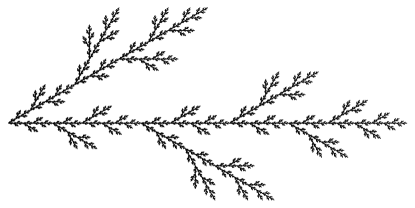
Figure 1. Hata tree set, with $\alpha=1/2+\sqrt{3}i/6$. The critical set consists of the point $|\alpha|^{2}=1/3$.

We will denote the points $\alpha,0$ and $1$ by $p_{0},p_{1}$ and $p_{2}$, respectively.

We observe that $K\setminus V_{0}$ is disconnected. We call $L$ the closure of the connected component of $K\setminus V_{0}$ that contains the interval $(0,1)$, and $M$ the closure of the component that contains the open segment from $0$ to $\alpha$.

If $w\in W_{m}$, we define $p_{wi}=F_{w}(p_{i})$, for $i=0,1,2$. We note that $p_{0}=p_{12}$, and that

$$|\alpha|^{2}=p_{10}=p_{21}.$$

As points in $V_{m}$, $m\geq 1$, we see that $p_{0}=p_{12\ldots 2}$, $p_{1}=p_{1\ldots 1}$ and $p_{2}=p_{2\ldots 2}$.

If $w\not=w^{\prime}$ are in $W_{m}$ and $p\in K_{w}\cap K_{w^{\prime}}$, then either

$$p=p_{w1}=p_{w^{\prime}0}\qquad\text{or}\qquad p=p_{w1}=p_{w^{\prime}2}.$$

We have the former case if $p\in V_{m}\setminus V_{m-1}$, and the latter if $p\in V_{m-1}$. If $p\in K_{w}$, and in no other $K_{w^{\prime}}$, then

$$p=p_{w0}\qquad\text{or}\qquad p=p_{w2}.$$

Again, we have the former case if $p\in V_{m}\setminus V_{m-1}$, and the latter if $p\in V_{m-1}$ (and $p\not=p_{1}$).

A point in $V_{m}$ has only one adyacent vertex if it’s of the form $p_{w20}$ or $p_{w22}$; otherwise it has three adyacent vertices in $V_{m}$, except for $p_{1}$, which has only two.

To construct a harmonic structure on the Hata set $K$, we need a Laplacian $D$ on $V_{0}$. Using the standard base $\{\chi_{\alpha},\chi_{0},\chi_{1}\}$, we set

$$D=\begin{pmatrix}-h&h&0\\ h&-(h+1)&1\\ 0&1&-1\end{pmatrix}.$$

Then, if $\mathbf{r}=(r_{1},r_{2})$, $(D,\mathbf{r})$ is a regular harmonic structure [Kig01] for $K$ if $h>1$,

$$r_{1}=\frac{1}{h}\qquad\text{and}\qquad r_{2}=1-\frac{1}{h^{2}}.$$

Explicitly, the Laplacian $H_{m}$ at a point $p\in V_{m}\setminus V_{0}$ is given by, if $p=p_{w1}=p_{w^{\prime}0}$,

(2.1a) $$\begin{split}H_{m}f(p)=\frac{1}{r_{w}}&\Big{(}f(p_{w2})-f(p_{w1})+h\big{(}f(p_{w0})-f(p_{w1})\big{)}\Big{)}\\ &+\frac{h}{r_{w^{\prime}}}\Big{(}f(p_{w^{\prime}1})-f(p_{w^{\prime}0})\Big{)};\end{split}$$

if $$p=p_{w1}=p_{w^{\prime}2}$$,

(2.1b) $$\begin{split}H_{m}f(p)=\frac{1}{r_{w}}&\Big{(}f(p_{w2})-f(p_{w1})+h\big{(}f(p_{w0})-f(p_{w1})\big{)}\Big{)}\\ &+\frac{1}{r_{w^{\prime}}}\Big{(}f(p_{w^{\prime}1})-f(p_{w^{\prime}2})\Big{)};\end{split}$$

if $$p=p_{w0}$$ and in no other cell,

(2.1c) $$H_{m}f(p)=\frac{h}{r_{w}}\Big{(}f(p_{w1})-f(p_{w0})\Big{)};$$

and, if $$p=p_{w2}$$ and in no other cell,

(2.1d) $$H_{m}f(p)=\frac{1}{r_{w}}\Big{(}f(p_{w1})-f(p_{w2})\Big{)}.$$

The Laplacian at the points $p_{0}$ and $p_{2}$ is given by formula (2.1d) for $m\geq 1$, while for $p=p_{1}$ is given by

$$H_{m}f(p)=\frac{1}{r_{w}}\Big{(}f(p_{w2}-f(p_{w1})+h\big{(}f(p_{w0})-f(p_{w1})\big{)}\Big{)},$$

$w=(1,1,\ldots,1)\in W_{m}$ is the word with $m$ ones. Note that $r_{w}=r_{1}^{m}$.

Observe that we have a family of harmonic structures for $K$, parameterized by $h$. For each $h>1$, the Hausdorff dimension with respect to the effective resistance metric [Kig01] is the unique $d$ such that

$$\Big{(}\frac{1}{h}\Big{)}^{d}+\Big{(}1-\frac{1}{h^{2}}\Big{)}^{d}=1.$$

We note that, since $F_{1}$ and $F_{2}$ are affine linear contractions with constants $|\alpha|$ and $1-|\alpha|^{2}$, respectively, $d$ coincides with the Hausdorff dimension with respect to the Euclidean metric if $h=1/|\alpha|$, by Hutchinson theorem [Hut81].

3. Harmonic functions

A function $u$ on $V_{*}$ is harmonic if $H_{m}u(p)=0$ for any $p\in V_{m}\setminus V_{0}$. In this section we describe an algorithm to construct harmonic functions on $V_{*}$ from any boundary values on $V_{0}$.

We say that $T_{w}\subset V_{m}$ is a minimal cell in $V_{m}$, if $T_{w}$ a set of three vertices of the form $p_{w0}$, $p_{w1}$ and $p_{w2}$, with $w\in W_{m}$. As points in $V_{m+1}$, we have that

$$T_{w}=\{p_{w12},p_{w11},p_{w22}\},$$

and the “new points” in $V_{m+1}$, contained in $K_{w}$, are then $p_{w10}=p_{w21}$ and $p_{w20}$. In other words, $K_{w}\cap V_{m+1}$ is the union of the minimal cells in $V_{m+1}$

$$T_{w1}=\{p_{w10},p_{w11},p_{w12}\}\qquad\text{and}\qquad T_{w2}=\{p_{w20},p_{w21},p_{w22}\}$$

Given a harmonic function on $V_{m}$, we want to extend to a harmonic function on $V_{m+1}$. The extension from $T_{w}$ to $T_{w1}\cup T_{w2}$ is given by the following algorithm.

Algorithm 3.1.

Let $u$ be a harmonic function on $V_{m}$. If, for each $w\in W_{m}$, $T_{w}$ is a minimal cell in $V_{m}$, and we extend $u$ to $T_{w1}\cup T_{w2}$ with

(3.1a) $$u(p_{w10}) = \Big{(}1-\frac{1}{h^{2}}\Big{)}u(p_{w1})+\frac{1}{h^{2}}u(p_{w2}),$$

(3.1b) $$u(p_{w20}) = u(p_{w10}),$$

then $u$ is harmonic in $V_{m+1}$.

Proof.

With respect to the basis $\{\chi_{p_{12}},\chi_{p_{11}},\chi_{p_{22}},\chi_{p_{10}},\chi_{p_{20}}\}$, the matrix of $H_{1}$ is given by

$$H_{1}=\begin{pmatrix}-\dfrac{1}{r_{1}}&\dfrac{1}{r_{1}}&0&0&0\\ \dfrac{1}{r_{1}}&-\dfrac{1+h}{r_{1}}&0&\dfrac{h}{r_{1}}&0\\ 0&0&-\dfrac{1}{r_{2}}&\dfrac{1}{r_{2}}&0\\ 0&\dfrac{h}{r_{1}}&\dfrac{1}{r_{2}}&-\dfrac{h}{r_{1}}-\dfrac{1+h}{r_{2}}&\dfrac{h}{r_{2}}\\ 0&0&0&\dfrac{h}{r_{2}}&-\dfrac{h}{r_{2}}\end{pmatrix}.$$

Writing the matrix as

$$\begin{pmatrix}T&J^{t}\\ J&X\end{pmatrix},$$

where $T$ takes functions on $V_{0}$ to functions on $V_{0}$, $J$ functions on $V_{0}$ to functions on $V_{1}$, and $X$ functions on $V_{1}$ to functions on $V_{1}$, Theorem 2.1.6 in [Kig01] implies that, if $u$ is harmonic, then

$$u|_{V_{1}\setminus V_{0}}=-X^{-1}J(u|_{V_{0}}).$$

Multiplying the matrices, and by the compatibility of the sequence of $H_{m}$ [Kig01], we obtain the result. ∎

Algorithm 3.1 allows us to construct harmonic functions on the Hata set with arbitrary precision, with any particular value of the parameter $h$. Figure 2 shows examples of harmonic functions, with distinct boundary values and distinct values of $h$.

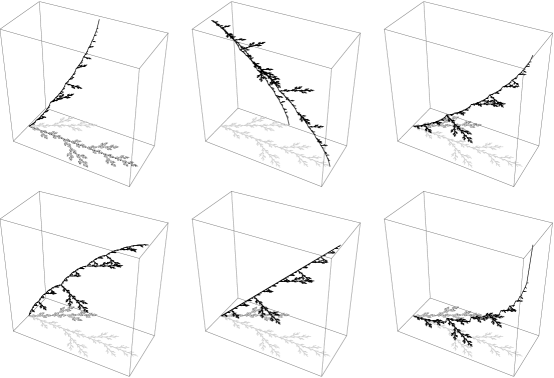
Figure 2. Harmonic functions on the Hata set. The three on the top correspond to $\alpha=1/2+\sqrt{3}i/6$ and $h=2$, with boundary values $\chi_{c}$, $\chi_{0}$ and $\chi_{1}$, respectively. On the bottom, harmonic funcions with boundary values $\chi_{1}$, with values of $h$ equal to $3/2$, $\sqrt{3}$ and $3$, respectively.

We observe that, since $K\setminus V_{0}$ is disconnected, we have harmonic functions supported in each one of the connected components $L$ and $M$ of $K\setminus V_{0}$, as we see in Figure 2 for harmonic functions with boundary values $\chi_{1}$ and $\chi_{\alpha}$, respectively.

Moreover, from equation (3.1a), the value of a harmonic function on each point $p$ in the line segment from 0 to 1 only depends on its values on the adyacent points to $p$ in the same line, from a previous iteration. Thus, one can easily construct restrictions of such harmonic functions to the line segment, following the work of [DSV99]. Figure 3 shows examples of such restrictions with boundary values $\chi_{1}$.

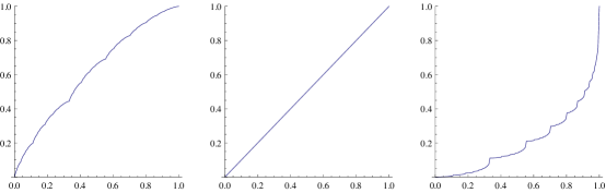
Figure 3. Restriction to $[0,1]$ of harmonic functions on the Hata set, with $\alpha=1/2+\sqrt{3}i/6$, boundary values $\chi_{1}$ and values of $h$ equal to $3/2$, $\sqrt{3}$ and $3$, respectively. Observe that, in the case $h=1/|\alpha|$, such restriction is a line. Otherwise, is a singular function.

We note, as readily verified from equation (3.1a), that the restriction of a harmonic function to this line segment is a line if $h=1/|\alpha|$, because the “middle” point in each iteration corresponds to the convex combination of its adyacent points in the line with weights $|\alpha|^{2}$ and $1-|\alpha|^{2}$. However, if $h\not=1/|\alpha|$, this restriction is a singular function, i. e. monotonic and with derivative 0 almost everywhere [YHK97].

Theorem 3.2.

Assume $h\not=1/|\alpha|$ and let $u$ be a harmonic function on the Hata set with boundary values $u|_{V_{0}}=\chi_{1}$, and let $f$ be its restriction to the interval $[0,1]$. Then

1. $f$ is increasing; and

2. $f$ is differentiable on $[0,1]\setminus V_{*}$, with

   $$f^{\prime}(x)=0$$

   for every $x\in[0,1]\setminus V_{*}$.

Proof.

Since $|\alpha|^{2}=p_{10}=F_{1}(F_{1}(1))$,

$$F_{1}(F_{1}(x))=|\alpha|^{2}x\qquad\text{and}\qquad F_{2}(x)=(1-|\alpha|^{2})x+|\alpha|^{2},$$

we see that equation (3.1a) implies that $f$ satisfies the system of equations

$$\begin{cases}f(x)=\dfrac{1}{h^{2}}f\bigg{(}\dfrac{1}{|\alpha|^{2}}x\bigg{)}&0\leq x\leq|\alpha|^{2}\vspace*{.05in}\\ f(x)=\bigg{(}1-\dfrac{1}{h^{2}}\bigg{)}f\bigg{(}\dfrac{1}{|\alpha|^{2}}x-1\bigg{)}+\dfrac{1}{h^{2}}&|\alpha|^{2}\leq x\leq 1.\end{cases}$$

Hence $f$ is essentially the same as Lebesgue’s singular function, and the result of the theorem follows as in [YHK97, Section 3.4]. ∎

We note that, if $h=1/|\alpha|$, then we have $f(x)=x$. Recall that $d$ coincides with the Euclidean Hausdorff dimension precisely when $h=1/|\alpha|$.

4. Laplacian

In this section we calculate the Laplacian $\Delta$ on the Hata set $K$ with respect to the self-similar measure $\mu$ with weights

$$\mu_{1}=\mu(F_{1}(K))=r_{1}^{d}=\Big{(}\frac{1}{h}\Big{)}^{d}\quad\text{and}\quad\mu_{2}=\mu(F_{2}(K))=r_{2}^{d}=\Big{(}1-\frac{1}{h^{2}}\Big{)}^{d}.$$

This measure is comparable to the Hausdorff measure with respect to the effective resistance metric [Kig94]. Moreover, $\mu$ is homogenous with respect to this metric [Sáe12].

As in [Kig01, Section 3.7], the domain $\mathcal{D}$ of the operator $\Delta$ is given by the set of continuous functions $u$ on $K$ such that there exists a continuous function $f$ with

(4.1) $$\lim_{m\to\infty}\max_{p\in V_{m}\setminus V_{0}}\big{|}\frac{1}{\mu_{p}^{m}}H_{m}u(p)-f(p)\big{|}=0,$$

where $\mu_{p}^{m}=\int_{K}\psi_{p}^{m}d\mu$, the integral of the $m$-harmonic spline $\psi_{p}^{m}$ that satisfies

$$\psi_{p}^{m}(p)=1\qquad\text{and}\qquad\psi_{p}^{m}(q)=0\text{ for }q\in V_{m},q\not=p.$$

If $u\in\mathcal{D}$ and $f$ is as in (4.1), then we write $\Delta u=f$. We can then approximate explicitly $\Delta u$ once we calculate the normalizing numbers $\mu_{p}^{m}$.

In order to calculate these numbers we observe that, by the self-similarity of $\mu$,

$$\begin{split}\mu_{p}^{m}&=\int_{K}\psi_{p}^{m}d\mu=\sum_{\begin{subarray}{c}w\in W_{m}\\ p\in K_{w}\end{subarray}}\int_{K_{w}}\psi_{p}^{m}d\mu\\ &=\sum_{\begin{subarray}{c}w\in W_{m}\\ p\in K_{w}\end{subarray}}\mu_{w}\int_{K}\psi_{F_{w}^{-1}(p)}^{0}d\mu=\sum_{\begin{subarray}{c}w\in W_{m}\\ p\in K_{w}\end{subarray}}\mu_{w}\mu_{F_{w}^{-1}(p)}^{0},\end{split}$$

where $\mu_{w}=\mu_{w_{1}}\cdots\mu_{w_{m}}$. Thus it is sufficient to calculate the three numbers $\mu_{\alpha}^{0},\mu_{0}^{0}$ and $\mu_{1}^{0}$ corresponding to $\alpha$, $0$ and $1$, the points in $V_{0}$.

Again, using the self-similarity of $\mu$, we observe that, by Algorithm 3.1

$$\int_{K}\psi_{\alpha}^{0}d\mu=\mu_{1}\int_{K}\psi_{1}^{0}d\mu,$$

$$\int_{K}\psi_{0}^{0}d\mu=\mu_{1}\int_{K}\bigg{(}\Big{(}1-\frac{1}{h^{2}}\Big{)}\psi_{\alpha}^{0}+\psi_{0}^{0}\bigg{)}d\mu\\ +\mu_{2}\int_{K}\bigg{(}\Big{(}1-\frac{1}{h^{2}}\Big{)}\psi_{\alpha}^{0}+\Big{(}1-\frac{1}{h^{2}}\Big{)}\psi_{0}^{0}\bigg{)}d\mu,$$

and

$$\int_{K}\psi_{1}^{0}d\mu=\mu_{1}\int_{K}\frac{1}{h^{2}}\psi_{\alpha}^{0}d\mu+\mu_{2}\int_{K}\Big{(}\frac{1}{h^{2}}\psi_{\alpha}^{0}+\frac{1}{h^{2}}\psi_{0}^{0}+\psi_{1}^{0}\Big{)}d\mu,$$

Thus, $\mu_{c}^{0}$, $\mu_{0}^{0}$ and $\mu_{1}^{0}$ satisfy the system of equations

$$\begin{split}\mu_{\alpha}^{0}&=\mu_{1}\mu_{1}^{0}\\ \mu_{0}^{0}&=\Big{(}1-\frac{1}{h^{2}}\Big{)}\mu_{\alpha}^{0}+\mu_{2}\Big{(}1-\frac{1}{h^{2}}\Big{)}\mu_{0}^{0}\\ \mu_{1}^{0}&=\frac{1}{h^{2}}\mu_{\alpha}^{0}+\frac{\mu_{2}}{h^{2}}\mu_{0}^{0}+\mu_{2}\mu_{1}^{0},\end{split}$$

where we have already use the fact $\mu_{1}+\mu_{2}=1$. Moreover, as the sum $\psi_{\alpha}^{0}+\psi_{0}^{0}+\psi_{1}^{0}$ is the constant function 1, we also have

$$\mu_{\alpha}^{0}+\mu_{0}^{0}+\mu_{1}^{0}=1.$$

Solving this system we obtain

$$\mu_{\alpha}^{0}=\frac{\mu_{1}\mu_{2}}{\mu_{1}\mu_{2}+(h^{2}-1)\mu_{1}+\mu_{2}},\quad\mu_{0}^{0}=\frac{(h^{2}-1)\mu_{1}}{\mu_{1}\mu_{2}+(h^{2}-1)\mu_{1}+\mu_{2}},$$

and

$$\mu_{1}^{0}=\frac{\mu_{2}}{\mu_{1}\mu_{2}+(h^{2}-1)\mu_{1}+\mu_{2}}.$$

5. Dirichlet Spectrum

We now proceed to study the Dirichlet spectrum of $\Delta$. As there is no decimation on the Hata set, we have to use the finite element method in order to approximate the eigenvalues and eigenfunctions of $\Delta$. We present a summary of the observations obtained numerically by solving the system of equations

$$\begin{cases}-\Delta_{m}u(x)=\lambda u(x)&x\in V_{m}\setminus V_{0}\\ u(p)=0&p\in V_{0},\end{cases}$$

where $\Delta_{m}u(x)=\frac{1}{\mu_{p}^{m}}H_{m}u(x)$.

Recall that $L$ is the closure of the connected component of $K\setminus V_{0}$ that contains the interval $(0,1)$, and $M$ the closure of the component that contains the open segment from $0$ to $\alpha$. Thus, linearly independent Dirichlet eigenfunctions are supported either in $L$ or $M$.

We observe numerically that the Dirichlet ground state is supported in $L$, as observed in Figure 4 (for $h=2$), corresponding to $\lambda_{1}\approx 9.888$.

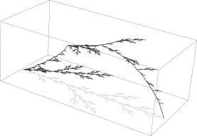
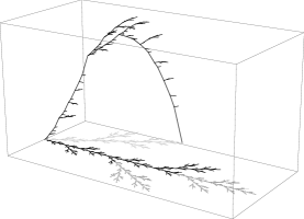
Figure 4. Dirichlet ground state $\phi$ for $h=2$, $\lambda_{1}\approx 9.888$, and its derived eigenfunction $\tilde{\phi}=\chi_{K_{1}}\cdot\phi\circ F_{1}^{-1}$, $\lambda_{3}\approx 56.21$, approximated to the eigth iteration, with $\alpha=1/2+\sqrt{3}i/6$. Note that $\phi$ is supported in $L$ and $\tilde{\phi}$ is supported in $M$.

For each eigenfunction $\phi$ supported in $L$, there is a corresponding eigenfunction supported in $M$.

Proposition 5.1.

Let $\phi$ be a Dirichlet eigenfunction of $\Delta$, supported in $L$, with respect to the eigenvalue $\lambda$. Then $\chi_{K_{1}}\cdot\phi\circ F_{1}^{-1}$ is an eigenfunction supported in $M$ with respect to the eigenvalue $\lambda/(r_{1}\mu_{1})$.

Proof.

Let $\tilde{\phi}=\chi_{K_{1}}\cdot\phi\circ F_{1}^{-1}$. If $x\in L$, then $x\in K_{2}$ or $x\in L\cap K_{1}$. In the first case, clearly $\tilde{\phi}(x)=0$ because $\chi_{K_{1}}(x)=0$, unless $x=|\alpha|^{2}$, the critical point. But in that case $x\in L\cap K_{1}$, and $F_{1}^{-1}(x)\in M$, so $\phi\circ F_{1}^{-1}(x)=0$ since $\phi$ is supported in $L$. Therefore $\tilde{\phi}$ is supported in $M$.

Now, for $u\in\mathcal{F}_{0}$, by the self-similarity of the Dirichlet form $\mathcal{E}$,

$$\begin{split}\mathcal{E}(\tilde{\phi},u)&=\frac{1}{r_{1}}\mathcal{E}(\tilde{\phi}\circ F_{1},u\circ F_{1})+\frac{1}{r_{2}}\mathcal{E}(\tilde{\phi}\circ F_{2},u\circ F_{1})\\ &=\frac{1}{r_{1}}\mathcal{E}(\phi,u\circ F_{1})=\frac{\lambda}{r_{1}}\int_{K}\phi\,u\circ F_{1}d\mu,\end{split}$$

where we have used the fact that $\tilde{\phi}$ is supported in $K_{1}$ and $\phi$ is a Dirichlet eigenfunction with respect to $\lambda$. One the other hand, by the self-similarity of the measure $\mu$,

$$\int_{K}\tilde{\phi}\,ud\mu=\mu_{1}\int_{K}\tilde{\phi}\circ F_{1}\,u\circ F_{1}d\mu+\mu_{2}\int_{K}\tilde{\phi}\circ F_{2}\,u\circ F_{2}d\mu=\mu_{1}\int_{K}\phi\,u\circ F_{1}d\mu,$$

so we obtain

$$\mathcal{E}(\tilde{\phi},u)=\frac{\lambda}{r_{1}\mu_{1}}\int_{K}\tilde{\phi}\,ud\mu,$$

and thus we conclude $\Delta\tilde{\phi}=-\dfrac{\lambda}{r_{1}\mu_{1}}\tilde{\phi}$. ∎

Figure 4 (right) shows the eigenfunction corresponding to the eigenvalue $\lambda_{3}=\lambda_{1}/r_{1}\mu_{1}\approx 56.21$, where $\lambda_{1}$ is the first Dirichlet eigenvalue ($h=2$). Proposition 5.1 lets us classify the Dirichlet eigenvalues (and eigenfunctions) in two classes, which we will call “primary” and “derived”. Table 1 shows the approximations to the first 20 Dirichlet eigenvalues, for $h=3/2,\sqrt{3}$ and $3$. We note that the derived eigenvalues appear in different positions in the sequence $\lambda_{k}$, depending on $h$, and they seem to be more sparse as $h$ increases.

Table 1. Approximations $\lambda_{k}^{10}$ to the first 20 Dirichlet eigenvalues for values of $h$ equal to $3/2$, $\sqrt{3}$ and $3$, indicating whether they correspond to a primary or a derived eigenfunction.

$h=3/2$		$h=\sqrt{3}$		$h=3$
$\lambda_{k}^{10}$	Type	$\lambda_{k}^{10}$	Type	$\lambda_{k}^{10}$	Type
2.12748	Primary	10.012	Primary	38.7802	Primary
5.80965	Derived	31.037	Primary	139.978	Primary
8.3776	Primary	38.7455	Derived	255.362	Primary
13.7502	Primary	83.3496	Primary	336.428	Primary
22.8762	Derived	106.366	Primary	435.129	Primary
33.3334	Primary	120.11	Derived	566.447	Primary
34.0196	Primary	193.982	Primary	741.34	Primary
37.5447	Derived	226.027	Primary	972.052	Primary
53.6119	Primary	244.389	Primary	1067.3	Derived
59.5265	Primary	322.541	Derived	1266.44	Primary
91.007	Derived	401.184	Primary	1623.74	Primary
92.8821	Derived	411.618	Derived	1814.55	Primary
98.8091	Primary	503.566	Primary	2248.34	Primary
109.503	Primary	580.894	Primary	2574.77	Primary
133.249	Primary	613.579	Primary	2909.76	Primary
136.474	Primary	654.576	Primary	3013.28	Primary
146.338	Derived	750.644	Derived	3299.2	Primary
162.469	Derived	783.032	Primary	3812.6	Primary
195.591	Primary	874.566	Derived	4001.01	Derived
213.997	Primary	945.709	Primary	4147.5	Primary

Figure 5 shows the first four Dirichlet eigenfunctions for those values of $h$, where we can observe the appearance of the derived eigenfunctions corresponding to $\lambda_{2}^{10}$ ($h=3/2$) and $\lambda_{3}^{10}$ ($h=\sqrt{3}$).

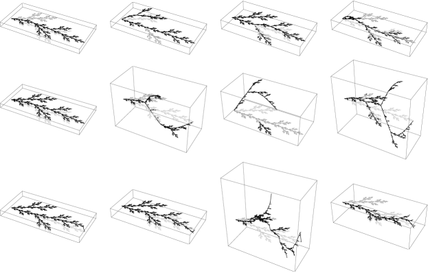
Figure 5. The first four Dirichlet eigenfunctions for the values $h=3/2,\sqrt{3}$ and $3$, respectively, approximated to the 10th iteration, with $\alpha=1/2+\sqrt{3}i/6$.

More interestingly, we show in Figure 6 the

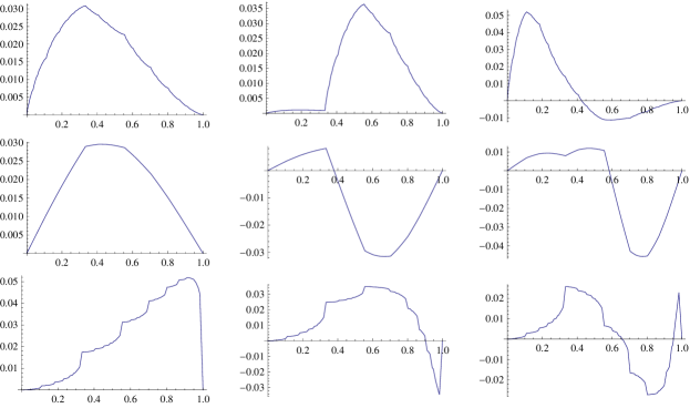
Figure 6. The restrictions to $[0,1]$ for the first three primary Dirichlet eigenfunctions for the values $h=3/2,\sqrt{3}$ and $3$, respectively, approximated to the 10th iteration, with $\alpha=1/2+\sqrt{3}i/6$.

restrictions of these eigenfunctions to the interval $[0,1]$ (only the primary ones, as the derived are zero in $[0,1]$). One can ask whether these functions have singularity properties as in the case of the harmonic functions.

Recall that, in the case of the harmonic functions, if $q\in V_{m+1}\cap[0,1]$ is the middle point between the points $x,y\in V_{m}\cap[0,1]$, then the harmonic function $u$ satisfies

(5.1) $$u(q)=(1-\theta)u(x)+\theta u(y),$$

where $\theta=1/h^{2}$. In Figure 7, we show the

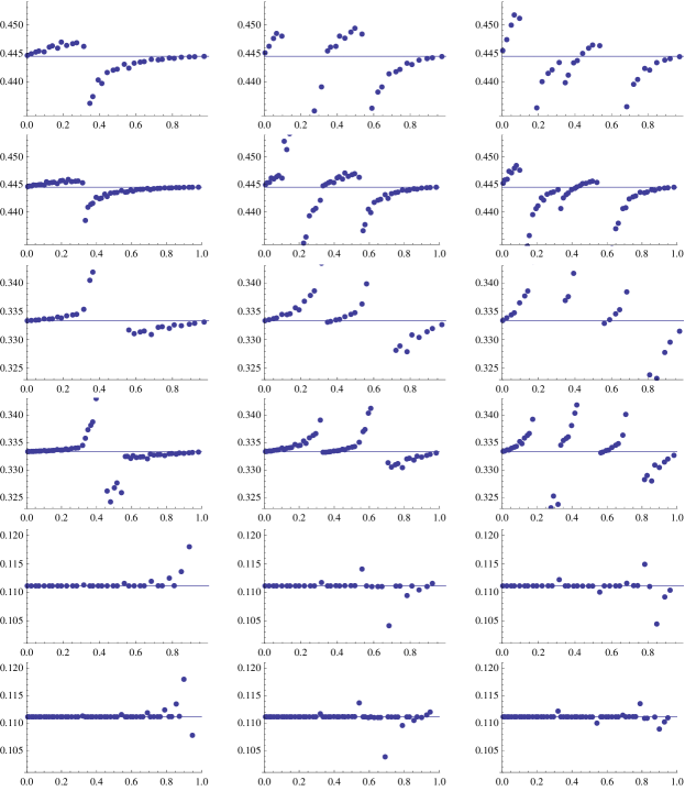
Figure 7. The values of $\theta$ that solve equation (5.1) for each middle point $q\in V_{9}\cap[0,1]$ (top of each pair of graphs) and $q\in V_{10}\cap[0,1]$ (bottom), for the approximations at $m=9$ and $m=10$ to the restrictions to $[0,1]$ for the first three primary Dirichlet eigenfunctions for the values $h=3/2,\sqrt{3}$ and $3$, respectively, with $\alpha=1/2+\sqrt{3}i/6$. The line corresponds to $1/h^{2}$, and the plot range is $1/h^{2}\pm.01$.

values of $\theta$ for such middle points $q\in V_{9}\cap[0,1]$ and $q\in V_{10}\cap[0,1]$, with respect to their adjacent points in $V_{8}$ and $V_{9}$, respectively, for the approximations at $m=9$ and $m=10$ to the restrictions to $[0,1]$ for the first three primary Dirichlet eigenfunctions for the values $h=3/2,\sqrt{3}$ and $3$.

We observe that they are closely equal to $1/h^{2}$, with better approximations as $h$ increases. We show the two iterations $m=9$ and $m=10$ in order to find out if the same proportions are preserved through two levels. As the $\theta$ are preserved through different iterations, we are lead to conjecture that the restrictions to $[0,1]$ of the Dirichlet eigenfunctions of the Laplacian with respect to $h\not=1/|\alpha|$ are singular functions whenever they are monotone, as in the case of the harmonic functions.

6. Conclusions

We have studied harmonic and Dirichlet eigenfunctions for the family of harmonic structures of the Hata set $K$ parametrized by $h>1$. The former can be constructed by means of the known algorithms for harmonic functions on PCF sets, and one observes that, when restricted to the interval $[0,1]$, the longest edge in $K$, one obtains singular functions for all but one value of the parameter $h$. In fact, we observed that the only value of $h$ for which these restrictions are not singular coincides with the value such that the Hausdorff dimensions of $K$ with respect to the Euclidean and effective resistance metrics are the same.

As is known, restrictions of harmonic functions to the edges of the Sierpinski gasket are also singular. This lead us to ask whether this behaviour is typical for harmonic functions on PCF sets. Moreover, since we know that in the case of the Hata set $K$ such functions are not singular for a particular embedding $K$ in the plane (given $h$, one can choose $\alpha$ such that $|\alpha|=1/h$), one can also ask whether, for every PCF set, there exists an embedding such that these restrictions are not singular. In particular, is this true for the Sierpinski gasket?

The same questions can be asked for the eigenfunctions of a PCF set. We have numerical evidence for the case of the Hata set, and one can start by studying those PCF sets with decimation. In particular, do the eigenfunctions on the Sierpinski gasket have singular restrictions to the edges?

References

- [ASST03] Bryant Adams, S. Alex Smith, Robert S. Strichartz, and Alexander Teplyaev, The spectrum of the Laplacian on the pentagasket, Fractals in Graz 2001, Trends Math., Birkhäuser, Basel, 2003, pp. 1–24. MR 2091699 (2006g:28017)
- [CSW11] Sarah Constantin, Robert S. Strichartz, and Miles Wheeler, Analysis of the Laplacian and spectral operators on the Vicsek set, Commun. Pure Appl. Anal. 10 (2011), no. 1, 1–44. MR 2746525 (2012b:28012)
- [DADCFS13] Enrique De Amo, Manuel Díaz Carrillo, and Juan Fernández Sánchez, Harmonic analysis on the Sierpiński gasket and singular functions, To appear in Acta Math. Hungar. (2013).
- [DDKÜ07] Bünyamin Demir, Vakif Dzhafarov, Şahin Koçak, and Mehmet Üreyen, Derivatives of the restrictions of harmonic functions on the Sierpinski gasket to segments, J. Math. Anal. Appl. 333 (2007), no. 2, 817–822. MR 2331696 (2009e:28031)
- [DSV99] Kyallee Dalrymple, Robert S. Strichartz, and Jade P. Vinson, Fractal differential equations on the sierpinski gasket, Journal of Fourier Analysis and Applications 5 (1999), 203–284, 10.1007/BF01261610.
- [Hat85] Masayoshi Hata, On the structure of self-similar sets, Japan J. Appl. Math. 2 (1985), no. 2, 381–414. MR 839336 (87g:58080)
- [Hut81] John E. Hutchinson, Fractals and self-similarity, Indiana Univ. Math. J. 30 (1981), no. 5, 713–747. MR 625600 (82h:49026)
- [Kig89] Jun Kigami, A harmonic calculus on the Sierpiński spaces, Japan J. Appl. Math. 6 (1989), no. 2, 259–290. MR 91g:31005
- [Kig93] by same author, Harmonic calculus on p.c.f. self-similar sets, Trans. Amer. Math. Soc. 335 (1993), no. 2, 721–755. MR 93d:39008
- [Kig94] by same author, Effective resistances for harmonic structures on p.c.f. self-similar sets, Math. Proc. Cambridge Philos. Soc. 115 (1994), no. 2, 291–303. MR 95h:28012
- [Kig01] by same author, Analysis on fractals, Cambridge University Press, Cambridge, 2001. MR 1 840 042
- [Sáe12] Ricardo A. Sáenz, Nontangential limits and Fatou-type theorems on post-critically finite self-similar sets, J. Fourier Anal. Appl. 18 (2012), no. 2, 240–265. MR 2898728
- [Shi91] Tadashi Shima, On eigenvalue problems for the random walks on the Sierpiński pre-gaskets, Japan J. Indust. Appl. Math. 8 (1991), no. 1, 127–141. MR 1093832 (92g:60094)
- [Str06] Robert S. Strichartz, Differential equations on fractals, Princeton University Press, Princeton, NJ, 2006, A tutorial. MR 2246975 (2007f:35003)
- [YHK97] Masaya Yamaguti, Masayoshi Hata, and Jun Kigami, Mathematics of fractals, American Mathematical Society, Providence, RI, 1997, Translated from the 1993 Japanese original by Kiki Hudson. MR 98j:28006