Abstract

The entanglement of different classes of initially entangled qubit pair is investigated in the presence of short laser pulses of rectangular and exponential shapes with either one or both qubits are excited. For the rectangular pulse, the detuning parameter protects the entanglement from degradation and controls its upper and lower bounds. We show that the upper bounds of entanglement decrease if both particles are excited, but the lower bounds are much better if only one particle is excited. The phenomena of entanglement degradation, sudden- death and -birth are shown for small initial time. Long -lived entanglement behavior, but with a variable degree, appears in the presence of rectangular pulse. However, in the case of the exponential pulse one obtains an invariably long- lived entanglement. For the combined case (rectangular $+$ exponential) , we show that one can generate a long-lived entanglement with small variable by increasing the strength of the rectangular pulse area and decreasing the Rabi frequency of the exponential pulse.

Keywords: Pulsed- driven qubits, Entanglement,

1 Introduction

One important research area within the context of quantum information science is investigating the dynamics of travelling states that are utilized to perform quantum information tasks as quantum teleportation and coding [1]. These states could be subject to noise channels [2, 3] or dissipative environment [4] and consequent interactions take place. These interactions may lead to undesirable loss of quantum entanglement (eq. decay and sudden- death ) that is essential for these states to perform in quantum information processing and computation [5, 6].

Non-dissipative single qubits when exposed to laser pulses have their energy levels splitting dependent on the pulse strength and its off-resonance parameter. Fourier and wavelet spectral features of the fluorescent radiation of such energy splitting have been investigated for various shapes of laser pulses ( [7]-[14]). Likewise, travelling quantum states that are exposed to pulsed lasers suffer a change in its entangled properties. Information transfer and orthogonality speed of a single qubit driven by a rectangular pulse has been recently investigated by us [15]. Recently it has been shown that quantum correlations can be enhanced and protected by applying a train of instantaneous pulses (so called bang-bang pulses) on a two qubit system [16]. Therefore, it is desirable to study the behavior of systems of a single qubit and two qubits when exposed to different shape of laser pulses.

In the present work, we investigate entangled properties of a class of generalized Werner state, including partial and maximum entangled states, interacting with two types of pulses, namely, rectangular and exponential pulses. Time evoluation of the initial state is obtained analytically for different cases and the the amount of the survival entanglement is quantified and computed accordingly.

The paper is organized as follows. In Sec.2, we present the model and its exact operator solution. The dynamics of entanglement is quantified in Sec.3, where we use the negativity as a measure of entanglement. The effect of the detuning parameter and the Rabi- frequency on the entanglement is investigated. Degree of entanglement in the three cases of pulse excitation of one or both particles, namely, rectangular, exponential and combination of them, is investigated in Sec.(3-5), respectively. A summary is given in Sec. 6.

2 The suggested Model

Assume that a source supplies two users, Alice and Bob, with a partially entangled (generalized Werner) state [17] defined by,

$$\rho=\frac{1}{4}(1+c_{xx}\sigma^{(a)}_{x}\sigma_{x}^{(b)}+c_{yy}\sigma_{y}^{(a1)}\sigma_{y}^{(b)}+c_{zz}\sigma_{z}^{(a)}\tau_{z}^{(b)}).$$ (1)

In (1) $a,b$ stand for Alice and Bob’s qubit, respectively. It assumed that during the transformation from the source to the users’ positions, each qubit interacts with a different pulse. The full Hamiltonian of this system, within the rotating wave approximations (in units of $\hbar=1$) is given by [9],

$$\hat{H}^{(j)}=\omega_{a}\hat{S}_{z}^{(j)}+\frac{\Omega^{(j)}(t)}{2}\Bigl{\{}\hat{S}_{+}^{(j)}e^{-i\omega^{(j)}_{l}t}+c.c)\Bigr{\}},$$ (2)

where $i=a$ (Alice qubit) and $i=b$ (Bob qubit), the spin-$\frac{1}{2}$ operators $\hat{S_{\pm}^{(i)}},\hat{S_{z}^{(j)}}$ obey the $Su(2)$ algebra,

$$[\hat{S}_{+}^{(j)},\hat{S}_{-}^{(j)}]=2\hat{S}_{z}^{(j)},\quad[\hat{S}_{z}^{(j)},\hat{S}_{\pm}^{(j)}]=\pm\hat{S}_{\pm}^{(j)}.$$ (3)

The parameter $\Omega^{(j)}(t)=\Omega_{0}^{(j)}f^{(j)}(t)$ where $\Omega^{(j)}$ represents the real Rabi frequency associated with the laser pulse and $f^{(j)}(t)$ is a dimensionless parameter describes the pulse shape. For the rectangular pulse this function is defined as

$$f^{(j)}(t)=\left\{\begin{array}[]{ll}1&\textrm{ for $t\in[0,T]$}\\ 0&\quad\textrm{otherwise},\\ \end{array}\right.$$ (4)

where the pulse duration $T$ is much shorter than the lifetime of the atomic upper state, hence atomic damping can be discarded. For the exponential pulse of widith $\gamma_{p}$ the function $f^{(i)}(t)$ is defined as [14]

$$f^{(j)}(t)=\left\{\begin{array}[]{ll}e^{-\gamma_{p}t}&\textrm{ for $t\geq 0$}\\ 0&\quad\textrm{for $t<0$}.\\ \end{array}\right.$$ (5)

To solve the system which is given by the equations (1,2), we introduce operators.

$$\hat{\sigma}_{\pm}^{(j)}(t)=\hat{S}^{(j)}_{\pm}(t)e^{\mp i\omega^{(j)}_{l}t},~{}\quad\hat{\sigma}^{(j)}_{z}(t)\equiv\hat{S}^{(j)}_{z}(t),$$ (6)

in the rotating frame where the $\hat{\sigma}$ operators obey the same algebraic form of Eq.(3). The time evolution of the operators $\hat{\sigma}_{\pm,z}(t)$ according to (2) are given by,

$$\hat{\sigma}^{(j)}_{x}(t) = \mathcal{A}^{(j)}_{x}(t)\hat{\sigma}_{x}(0)+\mathcal{A}^{(j)}_{y}(t)\hat{\sigma}_{y}(0)+\mathcal{A}^{(j)}_{z}(t)\hat{\sigma}_{z}(0),$$

$$\hat{\sigma}^{(j)}_{y}(t) = \mathcal{B}^{(j)}_{x}(t)\hat{\sigma}_{x}(0)+\mathcal{B}^{(j)}_{y}(t)\hat{\sigma}_{y}(0)+\mathcal{B}^{(j)}_{z}(t)\hat{\sigma}_{z}(0),$$

$$\hat{\sigma}^{(j)}_{z}(t) = \mathcal{D}^{(j)}_{x}(t)\hat{\sigma}_{x}(0)+\mathcal{D}^{(j)}_{y}(t)\hat{\sigma}_{y}(0)+\mathcal{D}^{(j)}_{z}(t)\hat{\sigma}_{z}(0),$$ (7)

where, the $c$-number time -dependent functions $\mathcal{A}_{i}(t),\mathcal{B}_{i}(t)$ and $\mathcal{D}_{i}(t)$ are given by

$$\mathcal{A}^{(j)}_{x}(t) = \frac{1}{2}\Bigl{[}\mathcal{C}^{(j)}_{+}(t)+\mathcal{C}^{(j)}_{-}(t)+c.c.\Bigr{]},\quad\mathcal{A}^{(j)}_{y}(t)=\frac{i}{2}\Bigl{[}\mathcal{C}^{(j)}_{+}(t)-\mathcal{C}^{(j)}_{-}(t)-c.c.\Bigr{]},\quad$$

$$\mathcal{A}^{(j)}_{z}(t) = \frac{1}{2}(\mathcal{C}^{(j)}_{z}(t)+c.c)$$

$$\mathcal{B}^{(j)}_{x}(t) = -\frac{i}{2}\Bigl{[}(\mathcal{C}^{(j)}_{+}(t)+\mathcal{C}^{(j)}_{-}(t)-c.c.)\Bigr{]},\quad\mathcal{B}^{(j)}_{y}(t)=i\mathcal{B}_{x}^{(j)}(t),\quad\mathcal{B}^{(j)}_{z}(t)=-i\mathcal{A}^{(j)}_{z}(t)$$

The expressions for the coefficients $\mathcal{C}^{(j)}_{\pm},\mathcal{C}^{(j)}_{z},D^{(j)}_{x},D^{(j)}_{y}$ and $D^{(j)}_{z}$ will be given below according to the type of the applied pulse. By using these results, the time evolution of the initial state (1) is given by

$$\rho_{ab}(t) = \frac{1}{4}\Bigl{[}1+\tilde{C}_{xx}\sigma^{(a)}_{x}\sigma_{x}^{(b)}+\tilde{C}_{xy}\sigma^{(a)}_{x}\sigma_{y}^{(b)}+\tilde{C}_{xz}\sigma^{(a)}_{x}\sigma_{z}^{(b)}+\tilde{C}_{yx}\sigma^{(a)}_{y}\sigma_{x}^{(b)}$$ (9)

$$+ \tilde{C}_{yy}\sigma^{(a)}_{y}\sigma_{y}^{(b)}+\tilde{C}_{yz}\sigma^{(a)}_{x}\sigma_{z}^{(b)}+\tilde{C}_{zx}\sigma^{(a)}_{z}\sigma_{x}^{(b)}+\tilde{C}_{zy}\sigma^{(a)}_{z}\sigma_{y}^{(b)}+\tilde{C}_{zz}\sigma^{(a)}_{z}\sigma_{z}^{(b)}\Bigr{]},$$

where, the nine coefficients $\tilde{C}_{kl}(t)$; $k,l=x,y,z$ are given by,

$$\tilde{C}_{kl}(t)=\mathcal{A}^{(1)}_{k}(t)\mathcal{A}^{(2)}_{l}(t)c_{xx}(0)+\mathcal{B}^{(1)}_{k}(t)\mathcal{B}^{(2)}_{l}(t)c_{yy}(0)+\mathcal{D}^{(1)}_{k}(t)\mathcal{D}^{(2)}_{l}(t)c_{zz}(0)$$ (10)

In the following two sections, we evaluate the time evolution of the initial state described by Eq.(1) for different types of pulses. we investigate the dynamics of entanglement of different classes of initial states. If we set $c_{xx}(0)=c_{yy}(0)=c_{zz}(0)=-1$, one gets the maximum entangled single state [18]. For the Werner state, $c_{xx}(0)=c_{yy}(0)=c_{zz}(0)=x$, which represents partially entangled states for $-\frac{1}{3}\leq x\leq\frac{1}{3}$ and seperable otherwise.

As for the dynamics of entanglement, we use the negativity as a measure of entanglement. This measure has been introduced by K. Zyczkowski et. al [20] and states that if the eigenvalues of the partial transpose of $\rho_{ab}(t)$, namely, $\rho_{ab}^{{}^{\mathsf{T}_{\!2}}}(t)$ are given by $\mu_{i};i=1,2,3,4,$ then the degree of entanglement (DOE) is given by,

$$\mathcal{E}(t)=\sum_{i=1}^{4}{\mu_{i}}-1,$$ (11)

where, $0<\mathcal{E}(t)<1$.

3 Rectangular Pulse Case

In this section we consider the effect of the rectangular pulse (4) on the degree of entanglement. In this case, the coefficients $\mathcal{C}^{(j)}_{\pm}(t),\mathcal{C}^{(i)}_{z}(t),D^{(j)}_{x}(t)$, $D^{(j)}_{y}(t)$ and $D^{(j)}_{z}(t)$ are given by, (cf [9]),

$$\mathcal{C}^{(j)}_{+}(t) = \frac{1}{2}\Bigl{\{}\left(\frac{\Omega^{(j)}}{\Omega^{(j)}_{1}}\right)^{2}+\left(\frac{\Delta^{2(j)}+\Omega_{1}^{2(j)}}{\Omega_{1}^{2(j)}}\right)\cos(\Omega_{1}^{(j)}t)\Bigr{\}}+i\frac{\Delta^{(j)}}{\Omega_{1}^{(j)}}\sin(\Omega_{1}^{(j)}t)$$

$$\mathcal{C}^{(j)}_{-}(t) = \frac{1}{2}\left(\frac{\Omega^{(j)}}{\Omega^{(j)}_{1}}\right)^{2}(1-\cos(\Omega_{1}^{(j))}t)),$$

$$\mathcal{C}^{(j)}_{z}(t) = \frac{\Delta^{(j)}\Omega^{(j)}}{(\Omega^{(j)}_{1})^{2}}\Bigl{(}1-\cos(\Omega^{(j)}_{1}t)\Bigr{)}-i\frac{\Omega^{(J)}}{\Omega_{1}^{(j)}}\sin(\Omega_{1}^{(j)}t)$$

$$D^{(j)}_{x}(t) = \frac{\Delta^{(j)}\Omega^{(j)}}{\Omega_{1}^{2(j)}}\Bigl{(}1-\cos(\Omega_{1}^{(j)}t)\Bigr{)},\quad D^{(j)}_{y}=\frac{\Omega^{(j)}}{\Omega_{1}^{(j)}}\sin(\Omega_{1}^{(j)}t),$$

$$D^{(j)}_{z}(t) = \Bigl{(}\frac{\Omega^{(j)}}{\Omega_{1}^{(j)}}\Bigr{)}^{2}\Bigl{[}\cos(\Omega_{1}^{(j)}t)+\Bigl{(}\frac{\Delta^{(j)}}{\Omega^{(j)}}\Bigr{)}^{2}\Bigr{]},$$ (12)

where $\Omega_{1}^{(j)}=\sqrt{(\Omega^{(j)}_{0})^{2}+(\Delta^{(j)})^{2}}$, $\Delta^{(j)}=\omega^{(j)}-\omega^{(j)}_{l}$.
Using Eqs.(9) and (12), one obtains the time evoluation of the initial density operator(1) in the presence of the local rectangular pulse. In this context, we investigate the effect of the detuning parameter $\Delta^{(j)}$ and the Rabi frequency $\Omega^{(j)}$ on the dynamics of the entanglement.

We consider three different initial states of the two non- interacting qubits:
(i) Maximum entangled state which is characteristed by $c_{xx}(0)=c_{yy}(0)=c_{zz}(0)=-1$. This state is defined as Bell state (singled state), $\rho_{\psi^{-}}=\bigl{|}\psi^{-}\bigr{\rangle}\bigl{\langle}\psi^{-}\bigr{|}$ where $\bigl{|}\psi^{-}\bigr{\rangle}=\frac{1}{\sqrt{2}}(\bigl{|}01\bigr{\rangle}-\bigl{|}10\bigr{\rangle})$,
(ii) Werner state, where we assume that $c_{xx}(0)=c_{yy}(0)=c_{zz}(0)=-0.9$, which represents a class of partially entangled states, and
(iii) Generalized Werner state, or $x-state$, where we assume that $c_{xx}(0)=-0.9,c_{yy}(0)=-0.8,$ and $c_{zz}(0)=-0.6$.

Having prepared the two qubit initially in any of the three aforementioned entangled states, we consider next two cases:

3.1 One driven-qubit

Here, we assume that only one qubit is driven by a rectangular pulse. This means we excite one qubit locally and then look globally for the entanglement of the whole system. We calculate the entanglement parameter $\mathcal{E}(T)$ at the end of the pulse duration $t=T$ and take the pulse area parameter $\Omega T/2\pi=n$ and define the normalized detuning $\Delta^{\prime(j)}=\Delta^{(j)}/\Omega$. At exact resonance $\Delta^{\prime(1)}=0$ (Fig.(1a)), $\mathcal{E}(T)$ keeps its initial values for integer values of (n), whilst for non-integer values of $(n)$ it is relatively reduced. For non-zero detuning , $\Delta^{\prime(1)}\neq 0$, Fig.(1b) shows that with increasing pulse area parameter $n=20$, $\mathcal{E}(T)$ approaches zero value with the initial generalized Werner state i.e., the less entangled initial state turns into separable state, while the maximum initial state (Bell-state) keeps the entanglement to non-zero lower bound. Further increase of $\Delta^{\prime(1)}$ causes increase in the lower bounds of entanglement increases for all initial states. Also, $\mathcal{E}(T)$ shows its periodic behaviour with further increase of (n).

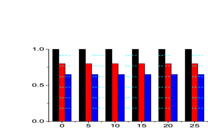
Figure 1: Degree of entanglement $\mathcal{E}(T)$, at the end of the rectangular pulse against the pulse area parameter $(n)$, where only one qubit is driven by the rectangular pulse. (a)$\Delta^{(1)}=0$, (b) $\Delta^{(1)}=1$

3.2 Two driven-qubit

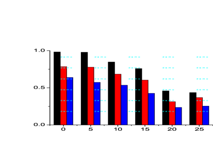
Figure 2: As Fig.(1) but with both qubits driven with rectangular pulses. (a) $\Delta^{(1)}=\Delta^{(2)}=0$, (b) $\Delta^{(1)}=\Delta^{(2)}=5$

When both qubits are driven by two resonant rectangular pulses, Fig.(2a) shows that, $\mathcal{E}(T)$ decreases( as compared with Fig.(1a)) as (n) increases to reach its lower bound. For non-resonant case ($\Delta^{(1)}=\Delta^{(2)}=5$), Fig.(2b) shows that the degree of entanglement between the two qubits decreases to reach their lower bounds. However for larger time, the degree of entanglement, $\mathcal{E}(T)$ increase to reach its upper bounds. The effect of changing the Rabi frequencies induces different oscillatory patterns.

4 Exponential Pulse Case

For resonant exponential pulse shape as defined in (5) the coefficients $\mathcal{C}^{(j)}_{\pm},\mathcal{C}^{(i)}_{z}\kappa^{(j)}_{y}$ and $\mathcal{D}^{j}_{x},\mathcal{D}^{(j)}_{y}$ and $\mathcal{D}_{z}^{(j)}$ are given by [14],

$$\mathcal{C}^{(j)}_{\pm} = \frac{1}{2}(1\pm\cos\lambda^{(j)}(t)),\quad\mathcal{C}^{(j)}_{z}=-i\sin{\lambda}^{(j)}(t)$$

$$D^{(j)}_{x} = 0,\quad D^{(j)}_{y}=\sin{\lambda}^{(j)}(t),\quad D^{(j)}_{z}=\cos{\lambda}^{(j)}(t),$$ (13)

where $\lambda^{(j)}(t)=\frac{\Omega^{(j)}}{\gamma^{(j)}_{p}}\Bigl{(}1-e^{-\gamma^{(j)}_{p}t}\Bigr{)}$. Here, we investigate the effect of the normalized Rabi frequency $\Omega^{\prime}=(\frac{\Omega}{\gamma_{p}})$ on the degree of entanglement between the two qubits if one or both of them are driven. Fig.(3) shows the behavior of $\mathcal{E}(T^{\prime})$; $T^{\prime}=\gamma_{p}t$, when only one particle is driven with an exponential pulse. It is clear that, for small values of the time $T^{\prime}\in[0,3]$, the entanglement $\mathcal{E}(T^{\prime})$ decreases fast to reach its lower bound. Also, the initial state with smaller degree of entanglement turns into a separable state. However, as $T^{\prime}$ increases further the degree of entanglement between the two particles doesn’t change. This means that we have a long lived entangled state with a fixed degree of entanglement. For larger values of Rabi frequency, $\Omega^{\prime}=10$, the number of oscillations on the time interval $T^{\prime}\in[0,1.9]$ increases and the phenomenon of sudden death and birth appear. However for larger time, the entanglement $\mathcal{E}$ re-birthes to reach its maximum values and then behaves invariably. All of these phenomena can be observed in Fig.(3b).

Fig.(4a) displays the behavior of $\mathcal{E}(T^{\prime})$, when both particles are locally pulsed with an exponential pulse. The attitude of the entanglement is similar to that shown in Fig.(3). However the entanglement doesn’t vanish and their lower bounds are larger than those shown in Fig.(3), where only one particle is driven. As the ratio $\Omega^{\prime}=(\frac{\Omega}{\gamma_{p}})$ increases, the number of oscillations increases. As the time increases further, the entanglement $\mathcal{E}(T^{\prime})$ increases to reach its upper bound and then behaves invariably.

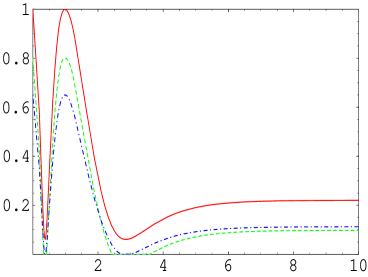
Figure 3: Degree of entanglement $\mathcal{E}(T^{\prime})$ against the normalized time $T^{\prime}=\gamma_{p}t$ in the case of of local exponential pulse with Rabi frequency $(\frac{\Omega}{\gamma_{p}})=5$(a), $(\frac{\Omega}{\gamma_{p}})=10$(b), where only one particle is driven. The solid curve, dot and dash-dot curves for systems prepared initially in maximum entangled state, partial entangled state with $c_{xx}=c_{yy}=c_{zz}=-0.9$ and $c_{xx}=-0.9,c_{yy}=-0.8,c_{zz}=-0.7$, respectively.

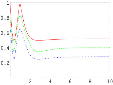
Figure 4: The same as Fig.(3) but with both particles are driven with exponential pulses.

5 Combined rectangular and exponential pulse case

In this section, we assume that Alice’s qubit is driven with a rectangular pulse as defined by (LABEL:RectPulse), while Bob’s qubit is driven with exponential pulse, (LABEL:ExpPulse). The dynamics of entanglement is displayed in Fig.(5), for different values of the pulses parameters. Fig.(5a) describes the behavior of the entanglement between the two qubits for $\omega^{(1)}=1$ and $(\frac{\Omega}{\gamma_{p}})=5$. It is clear that at $t=0$, the entanglement $\mathcal{E}=1$ for the maximum entangled state and $\mathcal{E}<1$ for the partially entangled states. The general behavior is similar to that depicted for the previous cases i.e., the degree of entanglement between the two qubits decay as $t$ increases. However the upper and lower bounds of $\mathcal{E}$ depends on the initial entanglement between the two qubits. Fig.(5b) displays the behavior of $\mathcal{E}$ for larger value of rectangular pulse strength i.e., we set $\Omega^{(1)}=2$, while we fix the strength of the exponential pulse. This behavior shows that the number of oscillations increases and the upper and lower bounds of entanglement increase. In Fig.(5c$\&5d$) we depict the behavior of the degree of entanglement between the two qubits for larger values of the exponential pulse, where we set $(\frac{\Omega}{\gamma_{p}})=10$. It is clear that the upper and lower bounds are much larger compared with those shown in Fig.(5a$\&5b$). However for system initially prepared in smaller degree of entanglement, the entanglement is temporary vanishes and rebirths again [21]

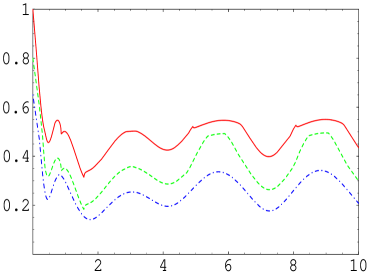
Figure 5: Degree of entanglement for a system initially prepared in maximum entangled state (solid-curve), Werner state (dot-curve) and generalized Werner state (dash-dot curve). It is assumed that, Alics’s qubit is driven with a rectangular pulse and Bob’s qubit is driven with an exponential pulse. We consider the resonant case i.e. $\Delta_{1}=\Delta_{2}=0$ and (a) $\Omega^{(1)}=1,(\frac{\Omega}{\gamma_{p}})=5$, (b) $\Omega^{(1)}=2,(\frac{\Omega}{\gamma_{p}})=5$, (c) $\Omega^{(1)}=1,(\frac{\Omega}{\gamma_{p}})=10$, (d) $\Omega^{(1)}=2,(\frac{\Omega}{\gamma_{p}})=10$.

From Fig.(5), one concludes that for small rectangular pulse area (i.e., small $\omega^{(1)}$) the phenomena of long -lived entanglement is remarkable. Increasing the number of oscillations (due to large pulse area) has a noticeable effect on the lower and upper bounds of entanglement. For larger values of Rabi frequency $\omega^{\prime}=\frac{\Omega}{\gamma_{p}}$ of the exponential pulse the upper and lower bounds increase larger than that shown for rectangular pulse. The phenomena of vanishing and re-birthing of entanglement is shown for larger values of $\omega^{\prime}$ in the case of exponential pulse.

6 Conclusion

Effects of rectangular and exponential pulse shapes on the entanglement between two initially entangled particles, maximally or partially, are discussed. We consider either one or both particles are driven. We show that, in the presence of the rectangular pulse the detuning parameter protect the degree of entanglement between the two particles from vanishing, where for the resonant case, the entanglement vanishes for small pulse time duration. Consequently, one can keep on a long - lived entanglement between the two particles. Although the upper bounds of the degree of entanglement between the two particles decrease as the detuning parameter increases, the lower bounds are improved. It is shown that, if only one particle is driven then the entanglement reaches its initial values by increasing the detuning paprmeter. However, if both particles are driven, then the upper bounds are always smaller than the initial one for larger values of the detning parameter. Rabi- oscillations have no effect on the lower and upper bounds of the survival amount of entanglement. However, the number of oscillations of the entanglement increases for larger values of Rabi-frequency, as expected.

In the presence of the exponential pulse, the phenomena of the sudden-death and -birth of entanglement appear for smaller time. On the other hand, for larger time, the long-lived entanglement is invariable. In this case, Rabi frequency plays an essential role on controlling the lower and upper bounds of entanglement. It is shown that, as one increases the Rabi frequency the entanglement is protected from being lost even for small intervals of time.

For the combined case, the long-lived entanglement is depicted for small strength values of the rectangular and exponential pulses. However, with larger strength of the exponential pulse, the upper bounds increase while the lower bounds of entanglement decreases and completely vanish for less initially entangled pairs. The oscillations of entanglement between its lower and upper bounds increase as the exponential pulse increases

In conclusion: one can protect the entanglement between two initially entangled particles by pulsed excitation of one or both particles. The rectangular pulse keeps a long-lived entanglement between the two particles, but with variable degree. On the other hand, excitation with the exponential pulse generates an invariable long-lived entanglement.

Acknowledgement The author (H A Batarfi) acknowledges the technical and financial support of (KAU)-grant No. (35-3-1432/HiCi).

References

- [1] S. M. Barnett,” Quantum Information” (Oxford Univ. Press, Oxford, 2009); Vlatko Vedral,”Introduction to Quantum information Science”, (Oxford Univ. Press, Oxford, 2008).
- [2] P. Huang, J. Zhu, G. He and G. Zeng, J. Phys. B:At. Mol Opt. Phys. 45 135501 (2012); M. Siomau, J. Phys. B:At. Mol Opt. Phys.45 035501 (2012).
- [3] N. Metwally Quantum Information Processing, 9 429 (2010); N. Metwally, J. Phys. A :Math. Theor.44 055305 (2011).
- [4] M. I. Hussain and M. Ikram, J. Phys. B:At. Mol Opt. Phys. 45 115503 (2012).
- [5] G. Lemos and F. Toscano, Phys. Rev. E 84, 016220 (2011).
- [6] Z. Liu and H. Fan, Phys. Rev. A 79, 064305 (2009).
- [7] P.A.Rodgers and S. Swain, Opt. Commu. 81 291 (1991).
- [8] A. Joshi and S. S. Hassan, J. Phys, B 35 1985 (2002).
- [9] S. S. Hassan, A. Joshi and N. M. M. Al-Madhari, J. Phys. B 41 145503 (2008); and corrigendum: J. Phys. B 42 089801 (2009).
- [10] S.S. Hassan, A. Joshi and H. A. Batarfi, Int. J. Theor. Physics, Group theory Nonlinear Optics, 13 371-382( 2010).
- [11] A. S. Mohamed, S. S. Hassan and M-A. Al-Saegh, Nonlinear Optics, Quantum Optics 36 107 (2007).
- [12] S. S. Hassan, M. A. Al-Saegh, A. S. Mohamed and H. A. Bararfi, Nonlinear Optics, Quantum Optics 42 37 (2011).
- [13] M. R. Qader, J. Assoc. Arab. Univ. for Basic Appl. Sci. 13 19 (2013)
- [14] H. A. Batrarfi, Nonlinear Opt. Phys. Materials, 21 1250025 (2012).
- [15] N. Metwally and S. S. Hassan, Nonlinear Opt. and Quantum Optics, 44 267 (2012).
- [16] H. Shi Xu and Jing-bo-Xu, Euro. Phys. Lett, 95 6003(2011); H. Shi Xu and Jing-bo-Xu, J. Opt. Soc. Amer. B 29 2074 (2012).
- [17] B. -G. Englert and N. Metwally, J. Mod. Opt, 47 221 (2000); B. -G. Englert and N. Metwally, Appl. Phys. B 72 35 (2001).
- [18] N. Metwally, Int. J. Theor. Phys. 49 1571 (2010).
- [19] A. Peres, Phys. Rev. Lett. 77, 1413 (1996); R. Horodecki, M. Horodecki and P. Horodecki, Phys. Lett. A222, 1 (1996).
- [20] K. Zyczkowski, P. Horodecki, A. Sanpera and M. Lewenstein, Phys. Rev. A 58, 883 (1998).
- [21] N. Metwally, M. Abdelaty and A.-S.F. Obada, Opt. Comm. 250 148 (2005).