Remote sensor response study in the regime of the microwave radiation-induced magnetoresistance oscillations

Tianyu Ye R. G. Mani Department of Physics and Astronomy, Georgia State University, Atlanta, Georgia 30303, USA W. Wegscheider Laboratorium für Festkörperphysik, ETH Zürich, 8093 Zürich, Switzerland

Abstract

A concurrent remote sensing and magneto-transport study of the microwave excited two dimensional electron system (2DES) at liquid Helium temperatures has been carried out using a carbon detector to remotely sense the microwave activity of the 2D electron system in the GaAs/AlGaAs heterostructure during conventional magneto-transport measurements. Various correlations are observed and reported between the oscillatory magnetotransport and the remotely sensed reflection. In addition, the oscillatory remotely sensed signal is shown to exhibit a power law type variation in its amplitude, similar to the radiation-induced magnetoresistance oscillations.

pacs:

The ultra-high-mobility two dimensional electron system (2DES) in GaAs/AlGaAs heterostructures exhibits giant oscillatory magnetoresistive response at liquid helium temperature in the form of Microwave-induced Zero-resistance States (MiZrS)Maninature2002 and Microwave-induced Magnetoresistance Oscillations (MIMOs)Maninature2002 ; ZudovPRLDissipationless2003 under photo-excitation. Such response is potentially useful for electromagnetic wave characterization in the technologically useful microwave and terahertz bands.ManiAPL2008 Thus, photo-excited magnetotransport has been extensively studied by experiment over the past decade.ManiPRBVI2004 ; ManiPRLPhaseshift2004 ; ManiEP2DS152004 ; KovalevSolidSCommNod2004 ; SimovicPRBDensity2005 ; ManiPRBTilteB2005 ; WiedmannPRBInterference2008 ; DennisKonoPRLConductanceOsc2009 ; ManiPRBPhaseStudy2009 ; ManiPRBAmplitude2010 ; ArunaPRBeHeating2011 ; ManiPRBPolarization2011 ; ManinatureComm2012 ; ManiPRBterahertz2013 ; TYe2013 As well, many theories have been developed to explain the MIMO’sDurstPRLDisplacement2003 ; AndreevPRLZeroDC2003 ; RyzhiiJPCMNonlinear2003 ; KoulakovPRBNonpara2003 ; LeiPRLBalanceF2003 ; DmitrievPRBMIMO2005 ; LeiPRBAbsorption+heating2005 ; InarreaPRLeJump2005 ; InarreaAPL2006 ; ChepelianskiiEPJB2007 ; InarreaAPL2008_2 ; InarreaAPL2008 ; InarreaAPL2009 ; FinklerHalperinPRB2009 ; ChepelianskiiPRBedgetrans2009 ; InarreaNanotech ; InarreaPRBPower2010 ; MikhailovPRBponderomotive2011 ; Inarrea2011 ; Inarrea2012 ; Inarrea2013 such as, for example, the displacement model that invokes radiation-assisted indirect inter-Landau-level scattering by phonons and impurities,DurstPRLDisplacement2003 ; RyzhiiJPCMNonlinear2003 ; LeiPRLBalanceF2003 the non-parabolicity model which considers non-parabolicity effects in an ac-driven system,KoulakovPRBNonpara2003 the inelastic model which explores the effects of a radiation-induced steady state non-equilibrium distribution,DmitrievPRBMIMO2005 and the radiation driven electron orbit model which follows the periodic motion of the electron orbit centers under irradiation.InarreaPRLeJump2005 The oscillatory minima of the MIMO’s are thought to transform into the experimentally observed zero-resistance states through either a current instability,AndreevPRLZeroDC2003 ; FinklerHalperinPRB2009 or from the accumulation/depletion of carriers at the contacts.MikhailovPRBponderomotive2011

Here, we use a remote sensing methodTYe2013 to further characterize MIMOs and study the evolution of the remotely sensed reflection signal and transport response with microwave frequency and microwave power, and compare the frequency and power dependence of the remote sensing signal with the magnetoresistive response of the 2DES. Our results also show a non-linear response vs. the microwave power in the oscillatory remotely sensed signal, similar to the observations of the non-linear oscillatory response observed in MIMOs.ManiPRBAmplitude2010

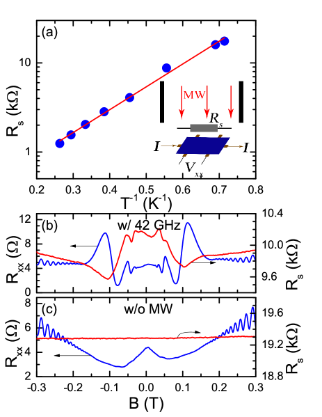
Refer to caption — Figure 1: (Color online) (a) The inset shows a sketch of our experiment set-up. This panel shows the response curve of the carbon sensor, $R_{s}$ . The red line shows that the sensor’s resistance increases rapidly with the reduction of the temperature. (b) and (c) exhibit sample’s diagonal resistance $R_{xx}$ (left ordinate) and sensor resistance $R_{s}$ (right ordinate) as functions of magnetic field, B, with (w/) and without (w/o) 42 GHz microwave excitation, respectively.

Experiments were carried out on high mobility GaAs/AlGaAs heterostructure Hall bar with gold-germanium contacts at liquid Helium temperatures. The specimen was mounted horizontally at the end of a sample probe and inserted into variable temperature insert inside the bore of superconducting solenoid. A base temperature of approximately 1.5 K was realized by pumping on the liquid helium within the variable temperature insert. Microwaves were sent by a launcher from the top of a circular microwave waveguide to the sample (Fig. 1(a) inset). A carbon remote sensor was placed above- and in close proximity to- the sample. This sensor exhibits a strong temperature coefficient, which is attributed to activated transport, in its response at liquid Helium temperatures, see Fig. 1 (a). After a brief illumination by a red Light-emitting diode to realize the high mobility condition, standard four terminal low frequency lock-in techniques were adopted to measure the sample signal and sensor signal concurrently.

The carbon sensor was found to be extremely effective in detecting small changes in the reflection associated with the MIMOs. As shown in Fig. 1 (b), with 42 GHz microwave illumination, the diagonal resistance $R_{xx}$ exhibits strong MIMOs within the magnetic field span $-0.15\leq B\leq+0.15$ Tesla, and the sensor resistance $R_{s}$ also reveals oscillatory response within the same regime. Without microwave excitation, both $R_{xx}$ and $R_{s}$ do not exhibit any oscillatory features, see Fig. 1(c), over the $-0.15\leq B\leq+0.15$ Tesla $B$ -span. Thus, $R_{s}$ oscillations are correlated with 2D electron transport induced by microwave excitation. As a consequence, the $R_{s}$ signal is adopted here to remotely sense the characteristics of MIMOs. It appears worth pointing out that with- or without- microwaves, the zero-field value of the magnetoresistance trace ( $R_{xx}$ )in 2DES is approximately the same. On the other hand, the remote sensor signal $R_{s}$ shifts by approximately 9 k $\Omega$ between the microwave on- and off- conditions. Such a large shift in $R_{s}$ is attributed to microwave heating, mostly due to the incident radiation. Thus, shifts in $R_{s}$ do not serve to characterize transport in the 2DES; it is only the oscillatory features on the $R_{s}$ traces that reflect the detector response to the microwave-induced transport in the 2DES.

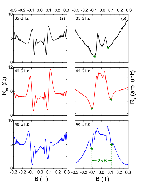
Fig. 2 exhibits $R_{xx}$ and $R_{s}$ responses to different microwave frequencies. Column (a) shows the $R_{xx}$ of the 2DES as the microwave frequency is increased from 35 GHz to 48 GHz. Note that MIMOs span a wider magnetic field regime as the microwave frequency, $f$ , increases because a larger Landau level splitting is required to obtain energy commensurability as the photon energy $hf$ increases. Column (b) shows the concurrently measured sensor resistance $R_{s}$ . Here, the oscillatory $R_{s}$ span a wider magnetic field as the microwave frequency increases, similar to MIMOs, see Fig. 2(a). At the same time, as the microwave frequency increases, more oscillatory structure appears in the $R_{s}$ , similar to MIMOs. At all the frequencies, there are discernable boundaries (marked by stars in Fig. 2 (b)), marking the $B$ -span for oscillatory $R_{s}$ . Further, a step-like response is apparent in the vicinity of the starred locations in Fig. 2(b). Such step-like remote sensor response is similar to the electron absorption reported by Iñarrea et al.InarreaNanotech . This feature suggests that the remote sensing signal is correlated to the response of the 2D electron system to microwave excitation.

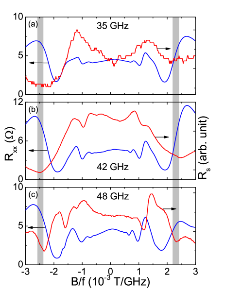
Figs. 3 (a) - (c) shows $R_{xx}$ and $R_{s}$ traces as functions of $B/f$ at three microwave frequencies. As the frequency increases, more MIMOs reveal themselves in the $R_{xx}$ trace. For instance, at 35 GHz, only three MIMOs appear for each direction of the magnetic field. At 48 GHz, at least four oscillations are discernable for each direction of the magnetic field. Note that, in this $B/f$ plot, the MIMO’s do not shift their positions on the abscissa as microwave frequency change. It is amazing that similar to the MIMOs, the turning points of $R_{s}$ on the abscissa also do not shift with the microwave frequency; they are fixed within the band $2.3\times 10^{-3}\leq B/f\leq 2.5\times 10^{-3}$ T/GHz, slightly above cyclotron resonance. For $|B/f|<2.3\times 10^{-3}$ T/GHz regime, the microwave energy, $hf$ , satisfies, $hf\geq\hbar\omega_{c}$ , allowing for radiation-induced inter-Landau-level transitions. Hence, the oscillatory remote sensor signal appears when radiation-induced inter-Landau-level transitions are allowed in the 2DES.

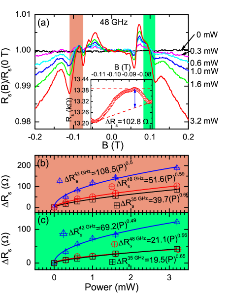
Using the above results, we have shown a correlation between MIMOs and the remotely sensed reflection signal. Below, we examine the evolution of oscillatory features in the reflection signal with the microwave power, see Fig. 4. Since the $R_{s}$ signal is also sensitive to the heating produced by the incident microwaves as mentioned previously, we plot zero-magnetic-field-normalized $R_{s}$ values, i.e., $R_{s}(B)/R_{s}(B=0)$ in Fig. 4(a) for the sake of presentation. In Fig. 4 (a), as the microwave power increase from 0 to 3.2 mW, the amplitude of oscillatory features in $R_{s}(B)/R_{s}(B=0)$ becomes larger, but their relative positions on the abscissa are fixed. We evaluated the amplitudes (without normalization) of the oscillatory features from the traces with different microwave powers. As indicated in Fig. 4(a), we measured the vertical height or amplitude from peak to the base line of one oscillation and plot these values as a function of microwave power in Fig. 4(c) and (d), respectively, for oscillatory features at negative and positive magnetic fields. The power dependence of the amplitude of oscillatory $R_{s}$ for all the frequencies could be fit with a power law function $\Delta R_{s}(f)=AP^{\alpha}$ , where $A$ and $\alpha$ are fit parameters that vary with the microwave frequency, see Fig. 4 (b) and (c). We found that the $\alpha$ value for every frequency was close to $1/2$ . Moreover, the $\alpha$ value for oscillatory features at postivie and negative magnetic fields are almost the same: 0.66 (- $B$ ) and 0.65 (+ $B$ ) for 35 GHZ; 0.5 (- $B$ ) and 0.49 (+ $B$ ) for 42 GHz; and 0.59 (- $B$ ) and 0.56 (+ $B$ ) for 48 GHz.

Both the frequency and power dependence of the remotely sensed reflection signal suggest that the remotely sensed reflection signal $R_{s}$ could serve to monitor in real-time the microwave induced transport in the GaAs/AlGaAs 2DES. In addition, the microwave power dependence measurements indicate a non-linear microwave power dependence of the remotely sensed signal $\Delta R_{s}$ , which agrees with the experimental report of the power dependence of $R_{xx}$ in the 2DESManiPRBAmplitude2010 . Indeed, both $R_{xx}$ and $\Delta R_{s}$ could be fit with the same power law function with exponent approximately equal to $1/2$ . Such agreement further supports the reliability of remotely sensing the microwave-induced transport in the 2DES.

Finally, we examine our results utilizing the radiation driven electron orbit modelInarreaPRLeJump2005 , because the simulations made with this model InarreaAPL2009 ; InarreaNanotech ; InarreaPRBPower2010 appear consistent with our results. In this model, radiation forces the electron orbit center to move back and forth in the direction of the radiation electric field at the frequency of radiation, and the $R_{xx}$ oscillations reflect the periodic motion of the electron orbit center. According to this model, the amplitude of diagonal resistance oscillations $R_{xx}\propto E_{0}$ , the amplitude of the microwave electric field. Since the radiation power $P=$ $1\over 2$ $c_{GaAs}\epsilon_{GaAs}\epsilon_{0}E_{0}^{2}$ , where $c_{GaAs}$ and $\epsilon_{GaAs}$ are the speed of light and dielectric constant in GaAs, and $\epsilon_{0}$ is the dielectric constant in vacuum, this theory asserts that the amplitude of oscillatory $R_{xx}\propto\sqrt{P}$ , implying an exponent of $1/2$ in plots such as Fig. 4(b) and Fig. 4(c), close to the experimentally observed value. Further, the microwave absorption model-simulation of this theory indicates a sharp change of the microwave absorption in 2DES in the vicinity of cyclotron resonance, which is consistent with the observations reported here in connection with figure 3.

In summary, we utilized a carbon sensor to remotely sense the photo-excited transport properties of 2D electrons in the regime of MIMOs. By changing the microwave frequency and power applied to the specimen, we deduced correlations between the observed magnetotransport in the 2DES and the remotely sensed reflection signal. We have also observed that oscillatory features in the remotely sensed reflection signal exhibit a non-linear amplitude variation with the microwave power, similar to the power-law type variation reported for the oscillatory diagonal resistance associated with MIMOs.

Basic research and helium recovery at Georgia State University is supported by the U.S. Department of Energy, Office of Basic Energy Sciences, Material Sciences and Engineering Division under DE-SC0001762. Additional support is provided by the ARO under W911NF-07-01-015.

References

(1) R. G. Mani, J. H. Smet, K. von Klitzing, V. Narayanamurti, W. B. Johnson, and V. Umansky, Nature 420, 646 (2002).
(2) M. A. Zudov, R. R. Du, L. N. Pfeiffer, and K. W. West, Phys. Rev. Lett. 90, 046807 (2003).
(3) R. G. Mani, Appl. Phys. Lett. 92, 102107 (2008).
(4) R. G. Mani, V. Narayanamurti, K. von Klitzing, J. H. Smet, W. B. Johnson, and V. Umansky, Phys. Rev. B 70, 155310 (2004); Phys. Rev. B 69, 161306 (2004).
(5) R. G. Mani, J. H. Smet, K. von Klitzing, V. Narayanamurti, W. B. Johnson, and V. Umansky, Phys. Rev. Lett. 92, 146801 (2004); Phys. Rev. B 69, 193304 (2004).
(6) R. G. Mani, Physica E 22, 1 (2004); Physica E. 25, 189 (2004).
(7) A. E. Kovalev, S. A. Zvyagin, C. R. Bowers, J. L. Reno, and J. A. Simmons, Solid State Commun. 130, 379 (2004).
(8) B. Simovič, C. Ellenberger, K. Ensslin, H. P. Tranitz, and W. Wegscheider, Phys. Rev. B 71, 233303 (2005).
(9) R. G. Mani, Phys. Rev. B 72, 075327 (2005); Appl. Phys. Lett. 91, 132103 (2007); Physica E40, 1178 (2008)
(10) S. Wiedmann, G. M. Gusev, O. E. Raichev, T. E. Lamas, A. K. Bakarov, and J. C. Portal, Phys. Rev. B 78, 121301 (2008).
(11) D. Konstantinov and K. Kono, Phys. Rev. Lett. 103, 266808 (2009).
(12) R. G. Mani, W. B. Johnson, V. Umansky, V. Narayanamurti, and K. Ploog, Phys. Rev. B 79, 205320 (2009).
(13) R. G. Mani, C. Gerl, S. Schmult, W. Wegscheider, and V. Umansky, Phys. Rev. B 81, 125320 (2010).
(14) A. N. Ramanayaka, R. G. Mani, and W. Wegscheider, Phys. Rev. B 83, 165303 (2011).
(15) R. G. Mani, A. N. Ramanayaka, W. Wegscheider, Phys. Rev. B 84, 085308 (2011); A. N. Ramanayaka, R. G. Mani, J. Iñarrea, and W. Wegscheider, Phys. Rev. B 85, 205315 (2012)..
(16) R. G. Mani, J. Hankinson, C. Berger, and W. A. de Heer, Nat. Commun. 3, 996 (2012).
(17) R. G. Mani, A. Ramanayaka, T. Ye, M. S. Heimbeck, H. O. Everitt and W. Wegscheider, Phys. Rev. B 87, 245308 (2013).
(18) T. Ye, R. G. Mani and W. Wegscheider, Appl. Phys. Lett. 102, 242113 (2013).
(19) A. C. Durst, S. Sachdev, N. Read, and S. M. Girvin, Phys. Rev. Lett. 91, 086803 (2003).
(20) A. V. Andreev, I. L. Aleiner, and A. J. Millis, Phys. Rev. Lett. 91, 056803 (2003).
(21) V. Ryzhii and R. Suris, J. Phys. Condens. Matter 15, 6855 (2003).
(22) A. A. Koulakov and M. E. Raikh, Phys. Rev. B 68, 115324 (2003).
(23) X. L. Lei and S. Y. Liu, Phys. Rev. Lett. 91, 226805 (2003).
(24) I. A. Dmitriev, M. G. Vavilov, I. L. Aleiner, A. D. Mirlin, and D. G. Polyakov, Phys. Rev. B 71, 115316 (2005).
(25) X. L. Lei and S. Y. Liu, Phys. Rev. B 72, 075345 (2005).
(26) J. Iñarrea and G. Platero, Phys. Rev. Lett. 94, 016806 (2005); Phys. Rev. B 76, 073311 (2007).
(27) J. Iñarrea and G. Platero, Appl. Phys. Letter 89, 052109 (2006).
(28) A. D. Chepelianskii, A. S. Pikovsky, and D. L. Shepelyansky, Eur. Phys. J. B 60, 225 (2007).
(29) J. Iñarrea, Appl. Phys. Lett. 92, 192113 (2008).
(30) J. Iñarrea and G. Platero, Appl. Phys. Letter 93, 062104 (2008).
(31) J. Iñarrea and G. Platero, Appl. Phys. Lett. 95, 162106 (2009).
(32) I. G. Finkler and B. I. Halperin, Phys. Rev. B 79, 085315 (2009).
(33) A. D. Chepelianskii, and D. L. Shepelyansky, Phys. Rev. B 80, 241308 (2009).
(34) J. Inarrea and G. Platero, Nanotechnology 21, 315401 (2010).
(35) J. Iñarrea, R. G. Mani and W. Wegscheider, Phys. Rev. B 82, 205321 (2010).
(36) S. A. Mikhailov, Phys. Rev. B 83, 155303 (2011).
(37) J. Iñarrea, Appl. Phys. Lett. 99, 232115 (2011).
(38) J. Iñarrea, Appl. Phys. Lett. 100, 242103 (2012).
(39) J. Iñarrea, Nano. Res. Lett. 8, 259 (2013).

Figure Captions

Figure 1: (Color online)(a) This panel shows the response curve of carbon sensor. The red line shows that the sensor’s resistance increases rapidly with the reduction of the temperature. The inset shows a sketch of our experiment set-up. (b) and (c) exhibit sample’s diagonal resistance $R_{xx}$ (left ordinate) and sensor resistance $R_{s}$ (right ordinate) as functions of magnetic field, B, with and without (w/o) 42 GHz microwave excitation.

Figure 2: (Color online) Column (a) shows the diagonal resistance, $R_{xx}$ , vs. the magnetic field, $B$ , for various microwave frequencies. Column (b) shows the corresponding sensor resistance, $R_{s}$ , vs. $B$ . From top to bottom, the microwave frequencies are 35 GHz, 42 GHz, and 48 GHz. Stars in column (b) mark the last major valley in the $R_{s}$ traces. Bottom panel of column (b) illustrates the determination of $2\Delta B$ .

Figure 3: (Color online) Panels (a) to (d) plot $R_{xx}$ (left scale) and $R_{s}$ (right scale) vs. $B/f$ for various microwave frequencies. Shadowed vertical bands mark the minima on $R_{s}$ traces.

Figure 4: (Color online) (a) This panel shows the power dependence of $R_{s}$ vs. $B$ under 48 GHz microwave excitation. All $R_{s}$ curves are normalized to their own zero magnetic field values. The inset of (a) illustrates the determination of the amplitude $\Delta R_{s}$ of the $R_{s}$ oscillation at 3.2 mW power in the brown area. The arrowed blue line indicates the $\Delta R_{s}$ associated with this oscillation. Panels (b) and (c) show plots of $\Delta R_{s}$ as functions of microwave power. Panel (b) corresponds to the oscillations in the brown shaded area in panel (a) and panel (c) corresponds to the green shaded area in panel (a). Different symbols indicate different frequencies: squares for 35 GHz, triangles for 42 GHz, and circles for 48 GHz. Power law functions are adopted to fit the symbols to solid lines. The fit results are also given in panels (b) and (c).