Classical Heisenberg spins with long-range interactions: Relaxation to equilibrium for finite systems

Abstract

Systems with long-range interactions often relax towards statistical equilibrium over timescales that diverge with $N$, the number of particles. A recent work [S. Gupta and D. Mukamel, J. Stat. Mech.: Theory Exp. P03015 (2011)] analyzed a model system comprising $N$ globally coupled classical Heisenberg spins and evolving under classical spin dynamics. It was numerically shown to relax to equilibrium over a time that scales superlinearly with $N$. Here, we present a detailed study of the Lenard-Balescu operator that accounts at leading order for the finite-$N$ effects driving this relaxation. We demonstrate that corrections at this order are identically zero, so that relaxation occurs over a time longer than of order $N$, in agreement with the reported numerical results.

Keywords: Kinetic theory of gases and liquids, Metastable states

1 Introduction

Long-range interacting systems are characterized by an interparticle potential with a range that is of the order of the system size. In $d$ dimensions, this corresponds to potentials decaying at large separation, $r$, as $1/r^{\alpha}$, where $\alpha$ lies in the range $0\leq\alpha\leq d$ [1, 2]. Examples include gravitational systems [3], plasmas [4], two-dimensional hydrodynamics [5], charged and dipolar systems [6], and many others.

Despite obvious differences, these systems often share a common phenomenology (see [1, 2]). In particular, the relaxation to equilibrium of an isolated long-range interacting system of $N$ particles proceeds in two steps: first, a collisionless relaxation, described by a Vlasov-type equation, brings the system close to a nonequilibrium state, called the ”quasistationary state” (QSS), whose lifetime increases with $N$; second, on timescales diverging with $N$, discreteness effects due to finite value of $N$ drive the system towards Boltzmann-Gibbs equilibrium. This second step is usually described by a Lenard-Balescu-type equation [7, 8]. This scenario is well established for plasmas and self-gravitating systems[9], and has been studied in detail in various toy models for long-range interactions [10, 11, 12, 13, 14]. The QSS lifetime, which may be regarded to be of the same order of magnitude as the relaxation time, is thus an important quantity: knowing it allows to distinguish between non-relaxed systems, which should be described by a QSS, and relaxed ones, for which collisional effects need to be taken into account and an equilibrium description may be relevant. This lifetime depends on the system under consideration. Kinetic theory usually predicts a QSS lifetime of order $N$, e.g., for 3d plasmas or 1d self-gravitating systems (see [15] for recent numerical tests), but this is not always the case; for example, the QSS lifetime is of order $N/\ln N$ for 3d self-gravitating systems [16]. Furthermore, it is known that the Lenard-Balescu collision term vanishes for 1d systems which do not develop any spatial inhomogeneity (see [17] for the 1d Coulomb case); one thus expects a relaxation time much longer than $N$ in these cases. This is indeed numerically observed, see [12], where a time of order $N^{1.7}$ is reported, and [18], where larger systems sizes are studied and the relaxation time is claimed to be of order $N^{2}$. A similar vanishing of the Lenard-Balescu operator has been found for point vortices in an axisymmetric configuration [19, 20, 21].

In a recent work, QSSs have been looked for and found in a dynamical setting different from the ones reviewed above, namely, in an anisotropic Heisenberg model with mean-field interactions [22]. Note that similar spin models with mean field interactions have been suggested to be relevant to describe some layered spin structures [23]. Specifically, the model in [22] comprises $N$ globally coupled three-component Heisenberg spins evolving under classical spin dynamics. An associated Vlasov-type equation is introduced, and QSSs are stationary solutions of this equation. In addition, numerical simulations for axisymmetric QSS suggest a QSS lifetime increasing superlinearly with $N$. In order to understand this observation analytically, we present in this work a detailed study of the Lenard-Balescu operator that accounts for leading finite-$N$ corrections of order $1/N$ to the Vlasov equation. With respect to 1D Hamiltonian systems, the spin dynamics introduces a new term in the Lenard-Balescu operator; it also complicates the analytical structure of the dispersion relation for the Vlasov-type equation. Nevertheless, we can still demonstrate that corrections at order $1/N$ are identically zero, so that relaxation occurs over a time longer than of order $N$, in agreement with the reported numerical results.

The paper is structured as follows. In section 2, we describe the model of study and its equilibrium phase diagram. As a step towards deriving the Vlasov equation to analyze the evolution of the phase space distribution in the limit $N\to\infty$, in section 3, we first write down the so-called Klimontovich equation; this leads to a derivation of the Vlasov equation and a discussion of a class of its stationary solutions in section 4. Section 5 contains our main results: it is devoted to the derivation of the Lenard-Balescu equation for our model of study, that is, the leading $1/N$ correction to the Vlasov equation; we show that this correction identically vanishes. In section 6, we consider an example of a Vlasov-stationary solution. In the energy range in which it is Vlasov stable, we demonstrate by performing numerical simulations of the dynamics that indeed its relaxation to equilibrium occurs over a timescale that does not grow linearly but rather superlinearly with $N$, in support of our analysis. The paper ends with conclusions.

2 The model

The model studied in Ref. [22] comprises $N$ globally coupled classical Heisenberg spins of unit length, denoted by ${\mathbf{S}}_{i}=(S_{ix},S_{iy},S_{iz})$, $i=1,2,\ldots,N$. In terms of spherical polar angles $\theta_{i}\in[0,\pi]$ and $\phi_{i}\in[0,2\pi]$, one has $S_{ix}=\sin\theta_{i}\cos\phi_{i},S_{iy}=\sin\theta_{i}\sin\phi_{i},S_{iz}=\cos\theta_{i}$. The Hamiltonian of the system is

$$H=-\frac{J}{2N}\sum_{i,j=1}^{N}{\bf S}_{i}\cdot{\bf S}_{j}+D\sum_{i=1}^{N}S^{2}_{iz}.$$ (1)

Here, the first term with $J>0$ describes a ferromagnetic mean-field coupling between the spins, while the second term is the energy due to a local anisotropy. We consider $D>0$, for which the energy is lowered by having the magnetization

$${\bf m}\equiv\frac{1}{N}\sum_{i=1}^{N}{\bf S}_{i}$$ (2)

pointing in the $xy$ plane. The coupling constant $J$ in equation (1) is scaled by $N$ to make the energy extensive [24], but the system is non-additive, implying thereby that it cannot be trivially subdivided into independent macroscopic parts, as is possible with short-range systems. In this work, we take unity for $J$ and the Boltzmann constant.

In equilibrium, the system (1) shows a continuous phase transition as a function of the energy density $e$, from a low-energy magnetized phase in which the system is ordered in the $xy$ plane to a high-energy non-magnetized phase, across a critical threshold given by [22]

$$e_{c}=D\Big{(}1-\frac{2}{\beta_{c}}\Big{)},$$ (3)

where the inverse temperature $\beta_{c}$ satisfies

$$\frac{2}{\beta_{c}}=1-\frac{1}{2\beta_{c}D}+\frac{e^{-\beta_{c}D}}{\sqrt{\pi\beta_{c}D}\mathrm{Erf}[\sqrt{\beta_{c}D}]}.$$ (4)

Here, $\mathrm{Erf}[x]=(2/\sqrt{\pi})\int_{0}^{x}{\rm d}t\leavevmode\nobreak\ e^{-t^{2}}$ is the error function.

The microcanonical dynamics of the system (1) is given by the set of coupled first-order differential equations

$$\frac{{\rm d}{\bf S}_{i}}{{\rm d}t}=\{{\bf S}_{i},H\};\leavevmode\nobreak\ \leavevmode\nobreak\ \leavevmode\nobreak\ \leavevmode\nobreak\ i=1,2,\ldots,N.$$ (5)

Here, noting that the canonical variables for a classical spin are $\phi$ and

$$u\equiv\cos\theta,$$ (6)

the Poisson bracket $\{A,B\}$ for two functions of the spins are given by $\{A,B\}\equiv\sum_{i=1}^{N}(\partial A/\partial\phi_{i}\partial B/\partial u_{i}-\partial A/\partial u_{i}\partial B/\partial\phi_{i})$, which may be rewritten as [25]

$$\{A,B\}=\sum_{i=1}^{N}{\bf S}_{i}\cdot\frac{\partial A}{\partial{\bf S}_{i}}\times\frac{\partial B}{\partial{\bf S}_{i}}.$$ (7)

Using equations (5) and (7), we obtain the equations of motion of the system as

$$\dot{S}_{ix}=S_{iy}m_{z}-S_{iz}m_{y}-2DS_{iy}S_{iz},$$ (8)

$$\dot{S}_{iy}=S_{iz}m_{x}-S_{ix}m_{z}+2DS_{ix}S_{iz},$$ (9)

$$\dot{S}_{iz}=S_{ix}m_{y}-S_{iy}m_{x},$$ (10)

where the dots denote derivative with respect to time. Summing over $i$ in equation (10), we find that $m_{z}$ is a constant of motion. The dynamics also conserves the total energy and the length of each spin. Using equations (8), (9), and (10), we obtain the time evolution of the variables $\theta_{i}$ and $\phi_{i}$ as

$$\dot{\theta_{i}} = m_{x}\sin\phi_{i}-m_{y}\cos\phi_{i},$$ (11)

$$\dot{\phi_{i}} = m_{x}\cot\theta_{i}\cos\phi_{i}+m_{y}\cot\theta_{i}\sin\phi_{i}-m_{z}+2D\cos\theta_{i}.$$ (12)

3 The Klimontovich equation

The state of the $N$-spin system is described by the discrete one-spin time-dependent density function

$$f_{d}(u,\phi,t)=\frac{1}{N}\sum_{i=1}^{N}\delta(u-u_{i}(t))\delta(\phi-\phi_{i}(t)),$$ (13)

which is defined such that $f_{d}(u,\phi,t){\rm d}u{\rm d}\phi$ counts the number of spins with its canonical coordinates in $[u,u+du]$ and $[\phi,\phi+d\phi]$. Here, $\delta$ is the Dirac delta function, $(u,\phi)$ are the Eulerian coordinates of the phase space, while $(u_{i},\phi_{i})$ are the Lagrangian coordinates of the spins. Note that $f_{d}$ satisfies $f_{d}(u,\phi,t)=f_{d}(u,\phi+2\pi,t)$ and the normalization $\int_{0}^{2\pi}{\rm d}\phi\int_{-1}^{1}{\rm d}u\leavevmode\nobreak\ f_{d}(u,\phi,t)=1$.

Differentiating $f_{d}$ with respect to time and using the equations of motion, (11) and (12), we get the Klimontovich equation for the time evolution of $f_{d}$ as

$$\frac{\partial f_{d}(u,\phi,t)}{\partial t}=-g_{u}\frac{\partial}{\partial u}f_{d}(u,\phi,t)-g_{\phi}\frac{\partial}{\partial\phi}f_{d}(u,\phi,t),$$ (14)

where

$$g_{u}\equiv g_{u}[f_{d}](u,\phi)$$

$$=\sqrt{1-u^{2}}(m_{y}[f_{d}]\cos\phi-m_{x}[f_{d}]\sin\phi),$$ (15)

$$g_{\phi}\equiv g_{\phi}[f_{d}](u,\phi)$$

$$=m_{x}[f_{d}]\frac{u}{\sqrt{1-u^{2}}}\cos\phi+m_{y}[f_{d}]\frac{u}{\sqrt{1-u^{2}}}\sin\phi-m_{z}[f_{d}]+2Du,$$ (16)

$$(m_{x},m_{y},m_{z})[f_{d}]$$

$$=\int_{0}^{2\pi}{\rm d}\phi\int_{-1}^{1}{\rm d}u\leavevmode\nobreak\ (\sqrt{1-u^{2}}\cos\phi,\sqrt{1-u^{2}}\sin\phi,u)f_{d}(u,\phi,t).$$ (17)

4 The Vlasov equation, and a class of stationary solutions

We now define an averaged one-spin density function $f_{0}(u,\phi,t)$, corresponding to averaging $f_{d}(u,\phi,t)$ over an ensemble of initial conditions close to the same macroscopic initial state. We write, quite generally, for an initial condition of the ensemble that

$$f_{d}(u,\phi,t)=f_{0}(u,\phi,t)+\frac{1}{\sqrt{N}}\delta f(u,\phi,t),$$ (18)

where, denoting by angular brackets the averaging with respect to the initial ensemble, we have $\langle f_{d}\rangle=f_{0}$. Here, $\delta f$ gives the difference between $f_{d}$, which depends on the given initial condition, and $f_{0}$, which depends on the average with respect to the ensemble of initial conditions.

Using equation (18) in equation (14), we get

$$\frac{\partial f_{0}}{\partial t}+g_{u}^{0}\frac{\partial f_{0}}{\partial u}+g_{\phi}^{0}\frac{\partial f_{0}}{\partial\phi}+\frac{1}{N}\Big{[}\delta g_{u}\frac{\partial\delta f}{\partial u}+\delta g_{\phi}\frac{\partial\delta f}{\partial\phi}\Big{]}$$

$$+\frac{1}{\sqrt{N}}\Big{[}\frac{\partial\delta f}{\partial t}+\delta g_{u}\frac{\partial f_{0}}{\partial u}+g_{u}^{0}\frac{\partial\delta f}{\partial u}+\delta g_{\phi}\frac{\partial f_{0}}{\partial\phi}+g_{\phi}^{0}\frac{\partial\delta f}{\partial\phi}\Big{]}=0,$$ (19)

where $g_{u}^{0}=g_{u}[f_{0}],g_{\phi}^{0}=g_{\phi}[f_{0}]$, and

$$\delta g_{u}=\sqrt{1-u^{2}}(m_{y}[\delta f]\cos\phi-m_{x}[\delta f]\sin\phi),$$ (20)

$$\delta g_{\phi}=m_{x}[\delta f]\frac{u}{\sqrt{1-u^{2}}}\cos\phi+m_{y}[\delta f]\frac{u}{\sqrt{1-u^{2}}}\sin\phi-m_{z}[\delta f].$$ (21)

We now average equation (19) with respect to the ensemble of initial conditions, and note that $\langle\delta f\rangle=0$ implies $\langle m_{x}[\delta f]\rangle=\langle m_{y}[\delta f]\rangle=\langle m_{z}[\delta f]\rangle=0$. Thus $\langle\delta g_{u}\rangle=\langle\delta g_{\phi}\rangle=0$, and we get

$$\frac{\partial f_{0}}{\partial t}+g_{u}^{0}\frac{\partial f_{0}}{\partial u}+g_{\phi}^{0}\frac{\partial f_{0}}{\partial\phi}=-\frac{1}{N}\Big{\langle}\delta g_{u}\frac{\partial\delta f}{\partial u}+\delta g_{\phi}\frac{\partial\delta f}{\partial\phi}\Big{\rangle}.$$ (22)

For finite times and in the limit $N\to\infty$ (or, for times $t\ll N$), we obtain the Vlasov equation satisfied by the averaged one-spin density function $f_{0}$ [26] as

$$\frac{\partial f_{0}}{\partial t}+g_{u}^{0}\frac{\partial f_{0}}{\partial u}+g_{\phi}^{0}\frac{\partial f_{0}}{\partial\phi}=0.$$ (23)

Note that the Vlasov equation has been formally obtained after averaging over an ensemble of initial conditions. However, if the fluctuations in the initial conditions are weak and do not grow too fast in time, we expect the Vlasov equation to also describe the time evolution of a single initial condition in the limit $N\to\infty$. This is put on firm mathematical grounds in [27, 28, 29], for systems with a standard kinetic energy and a regular enough interaction potential.

From equations (15), (16), and (17), it is clear that any distribution that does not depend on the angle $\phi$ (thus, axisymmetric about the $z$-axis) is a stationary solution of the Vlasov equation (23).

5 The Lenard-Balescu equation

We obtain in this section the main result of our paper: for model (1), the Lenard-Balescu operator, computed for stationary solutions of the Vlasov equation of the form $f_{0}(u)$, identically vanishes.

5.1 Formal derivation

The Lenard-Balescu equation describes the slow evolution of a stable stationary solution of the Vlasov equation under the influence of finite-$N$ corrections, at leading order in $1/N$ [26]. From equation (22), we get the Lenard-Balescu equation as

$$\frac{\partial f_{0}}{\partial t}=-\frac{1}{N}\Big{\langle}\delta g_{u}\frac{\partial\delta f}{\partial u}+\delta g_{\phi}\frac{\partial\delta f}{\partial\phi}\Big{\rangle},$$ (24)

where, subtracting equation (23) from equation (19), and keeping only the terms of order $1/\sqrt{N}$, we find that $\delta f$ follows the Vlasov equation linearized around its stable stationary solution $f_{0}$:

$$\frac{\partial\delta f}{\partial t}=\sqrt{1-u^{2}}\Big{[}\delta m_{x}\sin\phi-\delta m_{y}\cos\phi\Big{]}\frac{\partial f_{0}}{\partial u}-(2Du-m_{z}[f_{0}])\frac{\partial\delta f}{\partial\phi}.$$ (25)

Here, we have used $g_{\phi}^{0}=2Du-m_{z}[f_{0}]$ and $\delta m_{x,y}\equiv m_{x,y}[\delta f]$. Now, a natural timescale separation hypothesis greatly reduces the complexity of finding the solutions of the coupled system of PDEs, equations (24) and (25): The first of the two equations evolves on a slow $O(1/N)$ timescale, while the second one evolves on a fast $O(1)$ timescale. Then, we may first solve equation (25), and then use its solution to compute the right-hand side of (24) in the limit $t\to\infty$.

At this point, it is useful to make a comparison of our case with the standard case of particles with a kinetic energy moving in a classical potential, for example, a 1d system of particles with Coulomb interactions. The equivalent of the axisymmetric stationary solutions (independent of $\phi$) introduced in section  4 are the homogeneous solutions which depend only on velocity in this standard setting, so that the analog of $\delta g_{\phi}$ vanishes, whereas in our case of the spin dynamics, we have to deal with the extra term $\Big{\langle}\delta g_{\phi}\frac{\partial\delta f}{\partial\phi}\Big{\rangle}$.

5.2 Solution of the linearized Vlasov equation

We now solve equation (25) for $\delta f$, using Fourier-Laplace transforms

$$\delta f(u,\phi,t)=\sum_{k=-\infty}^{\infty}\int_{\Gamma}\frac{{\rm d}\omega}{2\pi}\widetilde{\delta f}_{k}(u,\omega)e^{i(k\phi-\omega t)},$$ (26)

$$\widetilde{\delta f}_{k}(u,\omega)=\int_{0}^{2\pi}\frac{{\rm d}\phi}{2\pi}\int_{0}^{\infty}{\rm d}t\leavevmode\nobreak\ \delta f(u,\phi,t)e^{-i(k\phi-\omega t)},$$ (27)

where the Laplace contour $\Gamma$ is a horizontal line in the complex-$\omega$ plane that passes above all singularities of $\widetilde{\delta f}_{k}(u,\omega)$.

We have

$$\delta m_{x}=\int_{\Gamma}\frac{{\rm d}\omega}{2\pi}e^{-i\omega t}\int_{-1}^{1}{\rm d}u\leavevmode\nobreak\ \pi\sqrt{1-u^{2}}\Big{(}\widetilde{\delta f}_{-1}(u,\omega)+\widetilde{\delta f}_{+1}(u,\omega)\Big{)},$$ (28)

$$\delta m_{y}=\int_{\Gamma}\frac{{\rm d}\omega}{2\pi}e^{-i\omega t}\int_{-1}^{1}{\rm d}u\leavevmode\nobreak\ \frac{\pi}{i}\sqrt{1-u^{2}}\Big{(}\widetilde{\delta f}_{-1}(u,\omega)-\widetilde{\delta f}_{+1}(u,\omega)\Big{)},$$ (29)

$$\delta m_{z}=m_{z}[\delta f]=\int_{\Gamma}\frac{{\rm d}\omega}{2\pi}e^{-i\omega t}\int_{-1}^{1}{\rm d}u\leavevmode\nobreak\ \pi u\widetilde{\delta f}_{0}(u,\omega),$$ (30)

so that equation (25) gives

$$\widetilde{\delta f}_{\pm 1}(u,\omega)=-\frac{\pi\sqrt{1-u^{2}}f_{0}^{\prime}(u)}{2Du-m_{z}[f_{0}]\mp\omega}\int_{-1}^{1}{\rm d}u^{\prime}\sqrt{1-u^{\prime 2}}\leavevmode\nobreak\ \widetilde{\delta f}_{\pm 1}(u^{\prime},\omega)$$

$$\mp\frac{i\delta f_{\pm 1}(u,0)}{2Du-m_{z}[f_{0}]\mp\omega},$$ (31)

where $f_{0}^{\prime}(u)=\partial f_{0}(u)/\partial u$ and $\delta f_{\pm 1}(u,0)$ is the Fourier transform of the initial fluctuations $\delta f(u,\phi,0)$. Multiplying both sides of the above equation by $\sqrt{1-u^{2}}$ and then integrating over $u$, we get

$$\epsilon_{\pm 1}(\omega)\int_{-1}^{1}{\rm d}u\sqrt{1-u^{2}}\leavevmode\nobreak\ \widetilde{\delta f}_{\pm 1}(u,\omega)=\mp i\int_{-1}^{1}{\rm d}u\frac{\sqrt{1-u^{2}}\delta f_{\pm 1}(u,0)}{2Du-m_{z}[f_{0}]\mp\omega},$$ (32)

where $\epsilon_{\pm 1}(\omega)$ is the so-called “Plasma response dielectric function” [26]:

$$\epsilon_{\pm 1}(\omega)=1+\pi\int_{LC}{\rm d}u\frac{(1-u^{2})f_{0}^{\prime}(u)}{2Du-m_{z}[f_{0}]\mp\omega}.$$ (33)

To make the dielectric function $\epsilon_{+1}$ (also, $\epsilon_{-1}$) analytic in the vicinity of the real axis (${\rm Im}(\omega)=0$), which will be needed for later purpose, the above integral has to be performed along the Landau contour shown in Fig. 1, as discussed in [26]; we have in this case

$$\epsilon_{\pm 1}(\omega)=\left\{\begin{array}[]{l}1+\pi\int_{LC}{\rm d}u\frac{(1-u^{2})f_{0}^{\prime}(u)}{2Du-m_{z}[f_{0}]\mp\omega};({\rm Im}(\omega)>0),\\ \\ 1+\pi{\rm P}\int_{LC}{\rm d}u\frac{(1-u^{2})f_{0}^{\prime}(u)}{2Du-m_{z}[f_{0}]\mp\omega}\\ \\ \pm i\frac{\pi^{2}}{2D}\left.(1-u^{2})f_{0}^{\prime}(u)\right|_{(m_{z}[f_{0}]\pm\omega)/(2D)};({\rm Im}(\omega)=0),\\ \\ 1+\pi\int_{LC}{\rm d}u\frac{(1-u^{2})f_{0}^{\prime}(u)}{2Du-m_{z}[f_{0}]\mp\omega}\\ \\ \pm i\frac{2\pi^{2}}{2D}\left.(1-u^{2})f_{0}^{\prime}(u)\right|_{(m_{z}[f_{0}]\pm\omega)/(2D)};({\rm Im}(\omega)<0),\\ \end{array}\right.$$

(40)

where ${\rm P}$ denotes the principal part. If $\omega\notin[-2D-m_{z}[f_{0}];2D-m_{z}[f_{0}]]$ (respectively, $\omega\notin[-2D+m_{z}[f_{0}];2D+m_{z}[f_{0}]]$), equation (33) already defines an analytic function $\epsilon_{+1}$ (respectively. $\epsilon_{-1}$) in the vicinity of a real $\omega$, without the need to take into account extra pole contributions as in (40). Note that $\epsilon_{\pm 1}(\omega)$ has two branch cut singularities on the real axis at $\omega=2D-m_{z}[f_{0}]$ and $\omega=-2D-m_{z}[f_{0}]$, which is the reason why these functions may be seen as multi-valued in the lower-half $\omega$-plane.

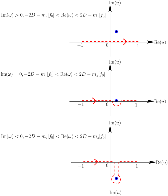
Figure 1: The Landau contour LC to evaluate $\epsilon_{+1}(\omega)$, shown as the dashed red line in the complex-$u$ plane.

Using equation (32) in equation (31) gives

$$\widetilde{\delta f}_{\pm 1}(u,\omega)=\pm\frac{i\pi\sqrt{1-u^{2}}f_{0}^{\prime}(u)}{\epsilon_{\pm}(\omega)[2Du-m_{z}[f_{0}]\mp\omega]}\int_{-1}^{1}{\rm d}u\frac{\sqrt{1-u^{2}}\delta f_{\pm 1}(u,\phi,0)}{2Du-m_{z}[f_{0}]\mp\omega}$$

$$\mp\frac{i\delta f_{\pm 1}(u,0)}{2Du-m_{z}[f_{0}]\mp\omega}.$$ (41)

We see from the above expression that the real pole at $\omega=\pm(2Du-m_{z}[f_{0}])$ is due to the free part of the evolution that does not involve interaction among the spins, and results in undamped oscillations of the fluctuations $\delta f(u,\phi,t)$, see equation (26). The other set of poles corresponds to the zeros of the dielectric function $\epsilon_{\pm}(\omega)$, i.e., values $\omega_{\rm p}$ (complex in general) that satisfy

$$\epsilon_{\pm 1}(\omega_{\rm p})=0.$$ (42)

Equation (26) implies that these poles determine the growth or decay of the fluctuations $\delta f(u,\phi,t)$ in time, depending on their location in the complex-$\omega$ plane. For example, when the poles lie in the upper-half complex $\omega$-plane, the fluctuations grow in time. On the other hand, when the poles are either on or below the real-$\omega$ axis, the fluctuations do not grow in time, but rather oscillate or decay in time, respectively. Then, the condition ensuring linear stability of a stationary solution of the Vlasov equation reads

$$\epsilon_{\pm 1}(\omega_{\rm p})=0\leavevmode\nobreak\ \Rightarrow\leavevmode\nobreak\ {\rm Im}(\omega_{\rm p})\leq 0.$$ (43)

The condition ${\rm Im}(\omega_{\rm p})=0$ corresponds to marginal stability.

To end this section, let us define for later use the quantities

$$\delta m_{\pm}\equiv\delta m_{x}\pm i\delta m_{y}.$$ (44)

On using equation (32), we get the corresponding Laplace transforms as

$$\widetilde{\delta m}_{+}(\omega)=\frac{2i\pi}{\epsilon_{-1}(\omega)}\int_{-1}^{1}{\rm d}u\frac{\sqrt{1-u^{2}}\delta f_{-1}(u,0)}{2Du-m_{z}[f_{0}]+\omega},$$ (45)

$$\widetilde{\delta m}_{-}(\omega)=-\frac{2i\pi}{\epsilon_{+1}(\omega)}\int_{-1}^{1}{\rm d}u\frac{\sqrt{1-u^{2}}\delta f_{+1}(u,0)}{2Du-m_{z}[f_{0}]-\omega}.$$ (46)

Equation (41) may now be expressed in terms of $\widetilde{\delta m}_{\pm}$ as

$$\widetilde{\delta f}_{+1}(u,\omega)=-\frac{\sqrt{1-u^{2}}f_{0}^{\prime}(u)}{2[2Du-m_{z}[f_{0}]-\omega]}\widetilde{\delta m}_{-}(\omega)-\frac{i\delta f_{+1}(u,0)}{2Du-m_{z}[f_{0}]-\omega},$$ (47)

$$\widetilde{\delta f}_{-1}(u,\omega)=-\frac{\sqrt{1-u^{2}}f_{0}^{\prime}(u)}{2[2Du-m_{z}[f_{0}]+\omega]}\widetilde{\delta m}_{+}(\omega)+\frac{i\delta f_{-1}(u,0)}{2Du-m_{z}[f_{0}]+\omega}.$$ (48)

5.3 Computing the Lenard-Balescu operator

We now compute the Lenard-Balescu operator, given by the right hand side of equation (24), in the limit $t\to\infty$, by using the results of the preceding subsection. We have

$$\Big{\langle}\delta g_{\phi}\frac{\partial\delta f}{\partial\phi}\Big{\rangle}=\sum_{k,l}\int_{\Gamma}\int_{\Gamma^{\prime}}\frac{{\rm d}\omega{\rm d}\omega^{\prime}}{4\pi^{2}}e^{i(k+l)\phi}e^{-i(\omega+\omega^{\prime})t}il\Big{\langle}\widetilde{\delta g}_{\phi,k}(u,\omega)\widetilde{\delta f}_{l}(u,\omega^{\prime})\Big{\rangle},$$ (49)

$$\Big{\langle}\delta g_{u}\frac{\partial\delta f}{\partial u}\Big{\rangle}=\sum_{k,l}\int_{\Gamma}\int_{\Gamma^{\prime}}\frac{{\rm d}\omega{\rm d}\omega^{\prime}}{4\pi^{2}}e^{i(k+l)\phi}e^{-i(\omega+\omega^{\prime})t}\Big{\langle}\widetilde{\delta g}_{u,k}(u,\omega)\frac{\partial\widetilde{\delta f}_{l}(u,\omega^{\prime})}{\partial u}\Big{\rangle}.$$ (50)

From equations (20) and (21), we have

$$\delta g_{\phi}=\Big{(}\frac{\delta m_{+}+\delta m_{-}}{2}\Big{)}\cos\phi\frac{u}{\sqrt{1-u^{2}}}+\Big{(}\frac{\delta m_{+}-\delta m_{-}}{2i}\Big{)}\sin\phi\frac{u}{\sqrt{1-u^{2}}}-\delta m_{z}[\delta f],$$

(51)

$$\delta g_{u}=\sqrt{1-u^{2}}\Big{[}\Big{(}\frac{\delta m_{+}-\delta m_{-}}{2i}\Big{)}\cos\phi-\Big{(}\frac{\delta m_{+}+\delta m_{-}}{2}\Big{)}\sin\phi\Big{]},$$ (52)

so that we have

$$\widetilde{\delta g}_{\phi,\pm 1}(u,\omega)=\widetilde{\delta m}_{\mp}(\omega)\frac{u}{2\sqrt{1-u^{2}}},\widetilde{\delta g}_{\phi,0}(u,\omega)=\widetilde{\delta m}_{z}(\omega),$$ (53)

$$\widetilde{\delta g}_{u,\pm 1}(u,\omega)=\mp\frac{\sqrt{1-u^{2}}}{2i}\widetilde{\delta m}_{\mp}(\omega).$$ (54)

From equations (45) and (46), we see that $\widetilde{\delta m}_{+}$ (respectively, $\widetilde{\delta m}_{-}$) depends on $\delta f_{-1}(u,0)$ (respectively, $\delta f_{+1}(u,0)$). Then, to compute the right hand hand side of equations (49) and (50), we need to evaluate averages of the type $\langle\delta f_{k}(u,0)\delta f_{l}(v,0)\rangle$ for the initial fluctuations at $t=0$. Note that $t=0$ as a notation is somewhat inappropriate, since actually this computation has to be repeated for any value of the slow time. We may assume that at $t=0$, the spins are almost independent (i.e., the two-spin correlation is of order $1/N$). In this case, one gets

$$\langle\delta f_{k}(u,0)\delta f_{l}(v,0)\rangle=\frac{\delta_{k,-l}}{2\pi}\left[f_{0}(u)\delta(u-v)+h(u,v)\right],$$ (55)

where $\delta_{k,-l}$ is the Kronecker delta function, and $h(u,v)$ is a smooth function. The precise form of this undetermined smooth function will play no role in the computation, as we will show below.

5.3.1 Computing $\Big{\langle}\delta g_{\phi}\frac{\partial\delta f}{\partial\phi}\Big{\rangle}$

Combining equations (53) and (55), we see that on the right hand side of equation (49), only the terms $(k=+1,l=-1)$ and $(k=-1,l=+1)$ give a non-zero contribution. We detail below the computation for the $(k=+1,l=-1)$ case, the other being similar. Note that $\Big{\langle}\delta g_{\phi}\frac{\partial\delta f}{\partial\phi}\Big{\rangle}$ is real; thus, we have to compute only the real part of the $(k=+1,l=-1)$ term, since its imaginary part must cancel with that of the $(k=-1,l=+1)$ term. In the following computation, we set $h(u,v)=0$; we will check at the end that indeed the contributions containing $h$ vanish.

We have

$$\langle\widetilde{\delta g}_{\phi,+1}(u,\omega)\widetilde{\delta f}_{-1}(u,\omega^{\prime})\rangle=-\frac{uf^{\prime}_{0}(u)}{4(2Du-m_{z}[f_{0}]+\omega^{\prime})}\langle\widetilde{\delta m}_{-}(\omega)\widetilde{\delta m}_{+}(\omega^{\prime})\rangle$$

$$+i\frac{u}{2\sqrt{1-u^{2}}(2Du-m_{z}[f_{0}]+\omega^{\prime})}\langle\widetilde{\delta m}_{-}(\omega)\delta f_{-1}(u,0)\rangle.$$ (56)

We thus need

$$\langle\widetilde{\delta m}_{-}(\omega)\widetilde{\delta m}_{+}(\omega^{\prime})\rangle$$

$$=\frac{2\pi}{\epsilon_{+1}(\omega)\epsilon_{-1}(\omega^{\prime})}\int_{-1}^{1}{\rm d}v\frac{(1-v^{2})f_{0}(v)}{(2Dv-m_{z}[f_{0}]-\omega)(2Dv-m_{z}[f_{0}]+\omega^{\prime})},$$ (57)

$$\langle\widetilde{\delta m}_{-}(\omega)\delta f_{-1}(u,0)\rangle=-i\frac{\sqrt{1-u^{2}}f_{0}(u)}{\epsilon_{+1}(\omega)(2Du-m_{z}[f_{0}]-\omega)},$$ (58)

where we have used equation (55). Using these equations in equation (56), we obtain

$$\langle\widetilde{\delta g}_{\phi,+1}(u,\omega)\widetilde{\delta f}_{-1}(u,\omega^{\prime})\rangle$$

$$=-\frac{\pi uf^{\prime}_{0}(u)}{2(2Du-m_{z}[f_{0}]+\omega^{\prime})\epsilon_{+1}(\omega)\epsilon_{-1}(\omega^{\prime})}$$

$$\times\int_{-1}^{1}{\rm d}v\frac{(1-v^{2})f_{0}(v)}{(2Dv-m_{z}[f_{0}]-\omega)(2Dv-m_{z}[f_{0}]+\omega^{\prime})}$$

$$+\frac{uf_{0}(u)}{2(2Du-m_{z}[f_{0}]+\omega^{\prime})(2Du-m_{z}[f_{0}]-\omega)\epsilon_{+1}(\omega)}$$

$$\equiv b_{1}+b_{2}.$$ (59)

Now, to compute the contribution to $\Big{\langle}\delta g_{\phi}\frac{\partial\delta f}{\partial\phi}\Big{\rangle}$ for ($k=+1,l=-1$), we have to integrate $b_{1}$ and $b_{2}$ over $\omega$ and $\omega^{\prime}$; we define

$$B_{1}\equiv\int_{\Gamma}\int_{\Gamma^{\prime}}\frac{{\rm d}\omega{\rm d}\omega^{\prime}}{4\pi^{2}}(-i)e^{-i(\omega+\omega^{\prime})t}b_{1},B_{2}\equiv\int_{\Gamma}\int_{\Gamma^{\prime}}\frac{{\rm d}\omega{\rm d}\omega^{\prime}}{4\pi^{2}}(-i)e^{-i(\omega+\omega^{\prime})t}b_{2}.$$ (60)

We want to compute $B_{1}$ and $B_{2}$ in the limit $t\to\infty$; thus, we will discard all terms decaying for large $t$.

Let us start with $B_{1}$. We have

$$B_{1}=i\frac{\pi uf_{0}^{\prime}(u)}{2}\int_{\Gamma^{\prime}}\frac{{\rm d}\omega^{\prime}}{2\pi}\frac{e^{-i\omega^{\prime}t}}{(2Du-m_{z}[f_{0}]+\omega^{\prime})(2Dv-m_{z}[f_{0}]+\omega^{\prime})\epsilon_{-1}(\omega^{\prime})}$$

$$\times\int_{\Gamma}\frac{{\rm d}\omega}{2\pi}e^{-i\omega t}\int_{-1}^{1}{\rm d}v\leavevmode\nobreak\ \frac{(1-v^{2})f_{0}(v)}{\epsilon_{+1}(\omega)(2Dv-m_{z}[f_{0}]-\omega)}.$$ (61)

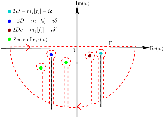
Figure 2: The $\Gamma$ contour to evaluate the integral in equation (62). Here, $\delta\to 0$ and $\delta^{\prime}\to 0$ are infinitesimal positive numbers. The thick vertical lines denote branch-cut singularities.

First, note that for large $t$,

$$\int_{\Gamma}\frac{{\rm d}\omega}{2\pi}\frac{e^{-i\omega t}}{\epsilon_{+1}(\omega)(2Dv-m_{z}[f_{0}]-\omega)}\sim i\frac{e^{-i(2Dv-m_{z}[f_{0}])t}}{\epsilon_{+1}(2Dv-m_{z}[f_{0}])},$$ (62)

which is obtained by deforming the $\Gamma$ contour into the ${\rm Im}(\omega)<0$ half-plane, see Fig. 2, and noting that due to the $e^{-i\omega t}$ factor, the only contribution to the contour integral in the limit $t\to\infty$ comes from the pole $2Dv-m_{z}[f_{0}]-i\delta^{\prime}$. Indeed, since $f_{0}$ is assumed stable, the zeros of $\epsilon_{+1}$, if any, have a negative imaginary part; their contributions thus decay exponentially in time. Similarly, the branch-cut singularities, see Fig. 2, contribute terms decaying algebraically in time. Note also that the important singularity at $2Dv-m_{z}[f_{0}]$ is real, and is in the range $[-2D-m_{z}[f_{0}];2D-m_{z}[f_{0}]]$. Then, according to the discussion in section 5.2, one needs to use the expression (40) for $\epsilon_{+1}$. The same remark applies to all the computations below, and we will not recall it each time.

The integration over $\omega^{\prime}$ in equation (61) is a bit more complicated, since there are two poles on the real axis, at $\omega^{\prime}=-2Du+m_{z}[f_{0}]$ and $\omega^{\prime}=-2Dv+m_{z}[f_{0}]$. With the same method as for $\omega$, we obtain

$$\int_{\Gamma^{\prime}}\frac{{\rm d}\omega^{\prime}}{2\pi}\frac{e^{-i\omega^{\prime}t}}{(2Du-m_{z}[f_{0}]+\omega^{\prime})(2Dv-m_{z}[f_{0}]+\omega^{\prime})\epsilon_{-1}(\omega^{\prime})}$$

$$=-i\left[\frac{e^{i(2Du-m_{z}[f_{0}])t}}{2D(v-u)\epsilon_{-1}(-2Du+m_{z}[f_{0}])}-\frac{e^{i(2Dv-m_{z}[f_{0}])t}}{2D(v-u)\epsilon_{-1}(-2Dv+m_{z}[f_{0}])}\right].$$ (63)

We finally get

$$B_{1}=i\frac{\pi uf_{0}^{\prime}(u)}{2}\int_{-1}^{1}{\rm d}v\leavevmode\nobreak\ \frac{(1-v^{2})f_{0}(v)}{\epsilon_{+1}(2Dv-m_{z}[f_{0}])}$$

$$\times\left\{\frac{e^{-i2D(v-u)t}}{2D(v-u)\epsilon_{-1}(-2Du+m_{z}[f_{0}])}-\frac{1}{2D(v-u)\epsilon_{-1}(-2Dv+m_{z}[f_{0}])}\right\}.$$ (64)

To perform the integral over $v$, we will use the following lemma.

Lemma:

$$\lim_{t\to\infty}\int_{-1}^{1}{\rm d}v\frac{\varphi(v)}{v-u}\left(\frac{e^{-i2D(v-u)t}}{\epsilon_{-1}(-2Du+m_{0})}-\frac{1}{\epsilon_{-1}(-2Dv+m_{0})}\right)=-i\pi\frac{\varphi(u)}{\epsilon_{-1}(-2Du+m_{0})}.$$ (65)

Proof:

$$\int_{-1}^{1}{\rm d}v\frac{\varphi(v)}{v-u}\left(\frac{e^{-i2D(v-u)t}}{\epsilon_{-1}(-2Du+m_{0})}-\frac{1}{\epsilon_{-1}(-2Dv+m_{0})}\right)$$

$$=\int_{-2D(1+u)t}^{2D(1-u)t}{\rm d}x\frac{\varphi(u+\frac{x}{2Dt})}{x}\left(\frac{e^{-ix}}{\epsilon_{-1}(-2Du+m_{0})}-\frac{1}{\epsilon_{-1}(-2Du+m_{0}-\frac{x}{t})}\right).$$ (66)

Recalling that $-1<u<1$, and taking the limit $t\to\infty$, the above expression simplifies to

$$\int_{-\infty}^{\infty}{\rm d}x\frac{\varphi(u)}{x}\left(\frac{e^{-ix}}{\epsilon_{-1}(-2Du+m_{0})}-\frac{1}{\epsilon_{-1}(-2Du+m_{0})}\right)$$

$$=\frac{\varphi(u)}{\epsilon_{-1}(-2Du+m_{0})}\int_{-\infty}^{\infty}{\rm d}x\frac{e^{-ix}-1}{x}.$$ (67)

The last integral is $-i\pi$, which completes the proof of the lemma.

Using the lemma, we conclude that

$$B_{1}=\frac{\pi^{2}uf_{0}^{\prime}(u)(1-u^{2})f_{0}(u)}{4D\epsilon_{+1}(2Du-m_{z}[f_{0}])\epsilon_{-1}(-2Du+m_{z}[f_{0}])}.$$ (68)

We now turn to the computation of $B_{2}$. The integration over $\omega$ and $\omega^{\prime}$ is performed as above, deforming the contours in the lower-half $\omega^{\prime}$-plane, and keeping only the contributions of the poles on the real axis. We obtain

$$B_{2} = -i\frac{uf_{0}(u)}{2}\frac{1}{\epsilon_{+1}(2Du-m_{z}[f_{0}])}$$ (69)

$$= -i\frac{uf_{0}(u)}{2}\frac{\epsilon_{-1}(-2Du+m_{z}[f_{0}])}{\epsilon_{+1}(2Du-m_{z}[f_{0}])\epsilon_{-1}(-2Du+m_{z}[f_{0}])}.$$

As explained above, we need to compute only the real part of $B_{2}$; thus, we keep only the contribution coming from the imaginary part of $\epsilon_{-1}(-2Du+m_{z}[f_{0}])$. Using from equation (40) that

$${\rm Im}[\epsilon_{-1}(-2Du+m_{z}[f_{0}])]=-\frac{\pi^{2}}{2D}(1-u^{2})f^{\prime}_{0}(u),$$ (70)

we conclude that

$${\rm Re}(B_{2})=-\frac{\pi^{2}uf_{0}(u)(1-u^{2})f^{\prime}_{0}(u)}{4D\epsilon_{+1}(2Du-m_{z}[f_{0}])\epsilon_{-1}(-2Du+m_{z}[f_{0}])}.$$ (71)

From equations (68) and (71), we find that $B_{1}+{\rm Re}(B_{2})=0$. Similar to above, one can show that the real part of the contribution to $\Big{\langle}\delta g_{\phi}\frac{\partial\delta f}{\partial\phi}\Big{\rangle}$ from ($k=-1,l=+1$) also vanishes, while, as discussed above, the imaginary part of the contribution to $\Big{\langle}\delta g_{\phi}\frac{\partial\delta f}{\partial\phi}\Big{\rangle}$ from ($k=-1,l=+1$) must cancel that from ($k=+1,l=-1$). So, we conclude that for our model,

$$\Big{\langle}\delta g_{\phi}\frac{\partial\delta f}{\partial\phi}\Big{\rangle}=0.$$ (72)

We need now to check that the contributions containing the function $h$ introduced in (55) indeed vanish. For example, let us compute its contribution to $B_{2}$. First, its contribution to $\langle\widetilde{\delta m}_{-}(\omega)\delta f_{-1}(u,0)\rangle$ is

$$-\frac{i}{\epsilon_{+1}(\omega)}\int_{-1}^{1}{\rm d}v\frac{\sqrt{1-v^{2}}}{2Dv-m_{z}[f_{0}]-\omega}h(v,u).$$ (73)

Thus, its contribution to $B_{2}$ is

$$\frac{u}{2\sqrt{1-u^{2}}}\int_{-1}^{1}{\rm d}v\sqrt{1-v^{2}}h(v,u)\int_{\Gamma}\int_{\Gamma^{\prime}}\frac{{\rm d}\omega{\rm d}\omega^{\prime}}{4\pi^{2}}e^{-i(\omega+\omega^{\prime})t}\frac{1}{\epsilon_{+1}(\omega)(2Dv-m_{z}[f_{0}]-\omega)}$$

$$\times\frac{1}{(2Du-m_{z}[f_{0}]+\omega^{\prime})}.$$ (74)

The integrals over $\omega$ and $\omega^{\prime}$ can be performed as before. Since the poles for $\omega$ and $\omega^{\prime}$ are different, we see that for large $t$, a factor $e^{-2Di(v-u)t}$ oscillating rapidly in time remains in the integral over $v$; this leads to this integral vanishing in the limit $t\to\infty$. A similar phenomenon ensures that all terms containing the function $h$ vanish in the same way. Thus, we set $h=0$ in the following, without modifying the results.

5.3.2 Computing $\Big{\langle}\delta g_{u}\frac{\partial\delta f}{\partial u}\Big{\rangle}$

As for $\Big{\langle}\delta g_{\phi}\frac{\partial\delta f}{\partial\phi}\Big{\rangle}$, we see that on the right hand side of equation (50), only the terms $(k=+1,l=-1)$ and $(k=-1,l=+1)$ are non-zero. We give below the computation for the case $(k=+1,l=-1)$ case, the other being similar. Again, we can restrict the computations to the real part of each term, since $\Big{\langle}\delta g_{u}\frac{\partial\delta f}{\partial u}\Big{\rangle}$ is real.

From equations (48) and (54), we get

$$\Big{\langle}\widetilde{\delta g}_{u,+1}(u,\omega)\frac{\partial\widetilde{\delta f}_{-1}(u,\omega^{\prime})}{\partial u}\Big{\rangle}$$

$$=\frac{\sqrt{1-u^{2}}}{4i}\frac{\partial}{\partial u}\Big{[}\frac{\sqrt{1-u^{2}}f_{0}^{\prime}(u)}{[2Du-m_{z}[f_{0}]+\omega^{\prime}]}\langle\widetilde{\delta m}_{-}(\omega)\widetilde{\delta m}_{+}(\omega^{\prime})\rangle\Big{]}$$

$$-\frac{1}{2}\sqrt{1-u^{2}}\frac{\partial}{\partial u}\Big{[}\frac{1}{2Du-m_{z}[f_{0}]+\omega^{\prime}}\langle\widetilde{\delta m}_{-}(\omega)\delta f_{-1}(u,0)\rangle\Big{]}$$

$$=\frac{\pi}{2i}\frac{\sqrt{1-u^{2}}}{\epsilon_{+1}(\omega)\epsilon_{-1}(\omega^{\prime})}\frac{\partial}{\partial u}\Big{[}\frac{\sqrt{1-u^{2}}f_{0}^{\prime}(u)}{[2Du-m_{z}[f_{0}]+\omega^{\prime}]}$$

$$\times\int_{-1}^{1}{\rm d}v\frac{(1-v^{2})f_{0}(v)}{(2Dv-m_{z}[f_{0}]-\omega)(2Dv-m_{z}[f_{0}]+\omega^{\prime})}\Big{]}$$

$$+\frac{i}{2}\frac{\sqrt{1-u^{2}}}{\epsilon_{+1}(\omega)}\frac{\partial}{\partial u}\Big{[}\frac{\sqrt{1-u^{2}}f_{0}(u)}{(2Du-m_{z}[f_{0}]+\omega^{\prime})(2Du-m_{z}[f_{0}]-\omega)}\Big{]}$$

$$\equiv a_{1}+a_{2},$$ (75)

where, in obtaining the second equality, we have used equations (57) and (58).

Now, to compute the contribution to $\Big{\langle}\delta g_{u}\frac{\partial\delta f}{\partial u}\Big{\rangle}$ for ($k=+1,l=-1$), we have to integrate $a_{1}$ and $a_{2}$ over $\omega$ and $\omega^{\prime}$. Let us define

$$A_{1}\equiv\int_{\Gamma}\int_{\Gamma^{\prime}}\frac{{\rm d}\omega{\rm d}\omega^{\prime}}{4\pi^{2}}e^{-i(\omega+\omega^{\prime})t}a_{1},A_{2}\equiv\int_{\Gamma}\int_{\Gamma^{\prime}}\frac{{\rm d}\omega{\rm d}\omega^{\prime}}{4\pi^{2}}e^{-i(\omega+\omega^{\prime})t}a_{2}.$$ (76)

We want to compute $A_{1}$ and $A_{2}$ in the limit $t\to\infty$, so that we may discard all terms decaying for large $t$.

Let us first compute $A_{1}$. Integration over $\omega$ and $\omega^{\prime}$ may be carried out by deforming the contours $\Gamma$ and $\Gamma^{\prime}$, as done in the preceding subsection. One gets

$$\int_{\Gamma}\frac{{\rm d}\omega}{2\pi}\frac{e^{-i\omega t}}{\epsilon_{+1}(\omega)(2Dv-m_{z}[f_{0}]-\omega)}=i\frac{e^{-i(2Dv-m_{z}[f_{0}])t}}{\epsilon_{+1}(2Dv-m_{z}[f_{0}])},$$ (77)

and

$$\int_{\Gamma^{\prime}}\frac{{\rm d}\omega^{\prime}}{2\pi}\frac{e^{-i\omega^{\prime}t}}{(2Du-m_{z}[f_{0}]+\omega^{\prime})(2Dv-m_{z}[f_{0}]+\omega^{\prime})\epsilon_{-1}(\omega^{\prime})}$$

$$=-i\Big{[}\frac{e^{i(2Du-m_{z}[f_{0}])t}}{2D(v-u)\epsilon_{-1}(-2Du+m_{z}[f_{0}])}-\frac{e^{i(2Dv-m_{z}[f_{0}])t}}{2D(v-u)\epsilon_{-1}(-2Dv+m_{z}[f_{0}])}\Big{]},$$ (78)

so that in the limit $t\to\infty$, we have

$$A_{1}=-i\frac{\pi}{2}\sqrt{1-u^{2}}\frac{\partial}{\partial u}\Big{[}\sqrt{1-u^{2}}f_{0}^{\prime}(u)\int_{-1}^{1}{\rm d}v\frac{(1-v^{2})f_{0}(v)}{2D(v-u)\epsilon_{+1}(2Dv-m_{z}[f_{0}])}$$

$$\times\Big{[}\frac{e^{-i2D(v-u)t}}{\epsilon_{-1}(-2Du+m_{z}[f_{0}])}-\frac{1}{\epsilon_{-1}(-2Dv+m_{z}[f_{0}])}\Big{]}\Big{]}$$

$$=-\frac{\pi^{2}}{4D}\sqrt{1-u^{2}}\frac{\partial}{\partial u}\Big{[}\frac{\sqrt{1-u^{2}}(1-u^{2})f_{0}(u)f_{0}^{\prime}(u)}{\epsilon_{+1}(2Du-m_{z}[f_{0}])\epsilon_{-1}(-2Du+m_{z}[f_{0}])}\Big{]},$$ (79)

where, in obtaining the second equality, we have used the lemma (65).

Now, $A_{2}$ may be computed along the same lines as done for $B_{2}$ in the preceding subsection. One gets

$${\rm Re}(A_{2})=\frac{i}{2}\sqrt{1-u^{2}}\frac{\partial}{\partial u}\Big{[}\frac{\sqrt{1-u^{2}}f_{0}(u)}{\epsilon_{+1}(2Du-m_{z}[f_{0}]}\Big{]}$$

$$=\frac{\pi^{2}}{4D}\sqrt{1-u^{2}}\frac{\partial}{\partial u}\Big{[}\frac{\sqrt{1-u^{2}}(1-u^{2})f_{0}(u)f_{0}^{\prime}(u)}{\epsilon_{+1}(2Du-m_{z}[f_{0}])\epsilon_{-1}(-2Du+m_{z}[f_{0}])}\Big{]},$$ (80)

where, in obtaining the second equality, we have used equation (70). From equations (79) and (80), we see that $A_{1}+{\rm Re}(A_{2})=0$. Similarly, one can show that the real part of the contribution to $\Big{\langle}\delta g_{u}\frac{\partial\delta f}{\partial u}\Big{\rangle}$ from ($k=-1,l=+1$) also vanishes, while the imaginary part of the contribution to $\Big{\langle}\delta g_{u}\frac{\partial\delta f}{\partial u}\Big{\rangle}$ from ($k=-1,l=+1$) must cancel that from ($k=+1,l=-1$). So, we conclude that for our model,

$$\Big{\langle}\delta g_{u}\frac{\partial\delta f}{\partial u}\Big{\rangle}=0.$$ (81)

Combining equations (72) and (81), we see that the Lenard-Balescu operator identically vanishes for our model, which is the announced result.

6 Example of a Vlasov-stationary state: Relaxation to equilibrium

In this section, let us consider as an example of an axisymmetric Vlasov stationary state $f_{0}$ a state prepared by sampling independently for each of the $N$ spins the angle $\phi$ uniformly over $[0,2\pi]$ and the angle $\theta$ uniformly over an interval of length $(a+b)$ asymmetric about $\theta=\pi/2$, that is, $\theta\in[\pi/2-a:\pi/2+b]$. The corresponding single-spin distribution is

$$f_{0}(u,\phi)=\frac{1}{2\pi}p(u),$$ (82)

with $p(u)$, the distribution for $u$, given by

$$p(u)=\left\{\begin{array}[]{ll}\frac{1}{\sin a+\sin b}&\mbox{if $u\in\left[-\sin b,\sin a\right]$},\\ &\\ 0&\mbox{otherwise}.\end{array}\right.\\$$ (83)

It is easily verified that this state has the energy

$$e=\Big{(}\frac{D}{3}-\frac{1}{8}\Big{)}(\sin^{2}a+\sin^{2}b)-\Big{(}\frac{D}{3}-\frac{1}{4}\Big{)}\sin a\sin b.$$ (84)

Since $m_{x}[f_{0}]=m_{y}[f_{0}]=0$, we have $g_{u}^{0}=0$, and also, $\partial f_{0}/\partial\phi=0$; it then follows that the state (82) is stationary under the Vlasov dynamics (23). Note that we have

$$m_{z}[f_{0}]=\frac{\sin a-\sin b}{2}.$$ (85)

As mentioned after equation (43), the condition ${\rm Im}(\omega_{\rm p})=0$ will correspond to the marginal stability of the state (82), so that the zeros $\omega_{\rm p}$ of the dielectric function lie on the real-$\omega$ axis. Let us denote these zeros as $\omega^{*}_{\rm pr}$. From equation (40), we find that $\omega^{*}_{\rm pr}$ satisfies

$$1+\pi{\rm P}\int_{-1}^{1}{\rm d}u\frac{(1-u^{2})f_{0}^{\prime}(u)}{2Du-m_{z}[f_{0}]\mp\omega^{*}_{\rm pr}}$$

$$\pm i\pi^{2}\left.(1-u^{2})f_{0}^{\prime}(u)\right|_{(m_{z}[f_{0}]\pm\omega^{*}_{\rm pr})/(2D)}=0.$$ (86)

Equating the real and the imaginary parts to zero, we get

$$1+\pi{\rm P}\int_{-1}^{1}{\rm d}u\frac{(1-u^{2})f_{0}^{\prime}(u)}{2Du-m_{z}[f_{0}]\mp\omega^{*}_{\rm pr}}=0,$$ (87)

$$\left.(1-u^{2})f_{0}^{\prime}(u)\right|_{(m_{z}[f_{0}]\pm\omega^{*}_{\rm pr})/(2D)}=0.$$ (88)

Now, equation (82) gives

$$f_{0}^{\prime}(u)=\frac{1}{2\pi(\sin a+\sin b)}[\delta(u+\sin a)-\delta(u-\sin b)],$$ (89)

so that we obtain from equation (88) that

$$\delta\Big{(}\frac{m_{z}[f_{0}]\pm\omega^{*}_{\rm pr}}{2D}+\sin a\Big{)}=\delta\Big{(}\frac{m_{z}[f_{0}]\pm\omega^{*}_{\rm pr}}{2D}-\sin a\Big{)},$$ (90)

implying that

$$\omega^{*}_{\rm pr}=-m_{z}[f_{0}].$$ (91)

Using equation (91) in equation (87), we get

$$4D=\frac{\cos^{2}a\leavevmode\nobreak\ \sin b+\cos^{2}b\leavevmode\nobreak\ \sin a}{\sin a\leavevmode\nobreak\ \sin b\leavevmode\nobreak\ (\sin a+\sin b)},$$ (92)

which when combined with equation (84) gives the energy

$$e=e^{*}=\frac{A}{B};$$

$$A=2(\sin a-\sin b)\leavevmode\nobreak\ \cos^{2}a+2\cot a\leavevmode\nobreak\ \sin^{2}b\leavevmode\nobreak\ \cos a+2\cos b\leavevmode\nobreak\ \cot b\leavevmode\nobreak\ \sin^{2}a$$

$$+2\cos^{2}b\leavevmode\nobreak\ (\sin b-\sin a)-3(\sin a-\sin b)^{2}(\sin a+\sin b),$$

$$B=24(\sin a+\sin b),$$ (93)

for which the state (82) is a marginally stable stationary solution of the Vlasov equation (23). For energies $e>e^{*}$, such a state is linearly stable under the Vlasov dynamics. On the basis of our analysis in this paper showing the Lenard-Balescu operator being identically zero, we expect that for finite $N$, the state relaxes to Boltzmann-Gibbs equilibrium on a timescale $\sim N^{\delta}$, with $\delta>1$. This was indeed observed in Ref. [22] for the class of initial states (82) that is non-magnetized, that is, $a=b$; in this case, combining equations (92) and (93), we get

$$e^{*}|_{a=b}=\frac{D}{3+12D}.$$ (94)

For energies $e<e^{*}|_{a=b}$, the state being linearly unstable under the Vlasov dynamics was seen to relax for finite $N$ to the Boltzmann-Gibbs equilibrium state over a timescale $\sim\ln N$ [22].

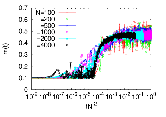
Figure 3: Magnetization $m(t)$ as a function of $tN^{-2}$ in the energy range in which the state (82) with $a=0.1,b=0.3$ is linearly stable under the Vlasov dynamics. Here, $e=0.22$, $D=8.224$, while the system sizes are marked in the figure. The figure suggests a relaxation timescale $\sim N^{\delta}$ with $\delta=2$, but the data do not allow a precise determination of the exponent $\delta$: any value of $\delta$ between about $1.7$ and $2$ is compatible with the data.

Let us choose $a=0.1,b=0.3$. Then, equation (93) gives $D\approx 8.224$, while equation (93) gives $e^{*}\approx 0.181$. Thus, for this value of $D$, the state (82) with $a=0.1,b=0.3$ is marginally stable under the linearized Vlasov dynamics at energy $e^{*}\approx 0.181$. Let us then choose a value of energy in the range $e^{*}<e<e_{c}$, where $e_{c}$ can be computed from equation (3) to be $e_{c}\approx 0.258$. We expect on the basis of the analysis presented in this paper that in this energy range, when the state (82) is Vlasov-stable, the relaxation to equilibrium should occur over a timescale that scales superlinearly with $N$. For $e=0.22$, results of numerical simulations of the dynamics shown in Fig. 3 indeed suggest a relaxation timescale $\sim N^{\delta}$, with $\delta>1$; for the range of system sizes explored in this numerical experiment, any value of $\delta$ between about $1.7$ and $2$ is compatible with the data.

7 Conclusions

In this paper, we have shown that the Lenard-Balescu operator identically vanishes for a system of globally coupled anisotropic Heisenberg spins, in an axially symmetric Vlasov-stable state. This result explains the numerical findings of [22], reporting a relaxation time for this system that scales superlinearly with $N$. To our knowledge, it is the first time that this kind of results has been obtained for a spin dynamics. This raises further questions, e.g., what are the general conditions to ensure that the Lenard-Balescu operator vanishes? The classical explanation relies on the structure of resonances between the particle trajectories: in the absence of resonances between particles with different momentum, the Lenard-Balescu operator should vanish. This heuristic argument applies to systems of particles moving in a 1d position space, thus with a 2d phase space, when the system is homogeneous [17, 30], implying a relaxation time growing superlinearly with $N$. This is also the case for axisymmetric configurations of point vortices [19, 20, 21], where the phase space is again two-dimensional. In a similar manner, it can be argued for the model we have studied that spins with different projections on the $z$-axis cannot exchange energy because they cannot be in resonance. In a sense, our precise computations validate this qualitative picture. However, recent numerical simulations of a model with a 4d phase space have also shown a relaxation time that appears superlinear in $N$ over the range of system sizes studied [14]: one would expect resonances to appear in this case. Thus, understanding the general conditions under which the Lenard-Balescu operator vanishes may still remain a partly open question.

One may also wonder how the relaxation occurs when the Lenard-Balescu operator vanishes. Formally, the Klimontovich expansion suggests that the next leading term is of order $1/N^{2}$. Although writing down this term is possible in principle, its evaluation is difficult. However, it is not quite clear that the expansion is valid over such long timescales.

Finally, let us stress that the standard route to a formal derivation of the Lenard-Balescu equation, as followed in this article, involves an averaging over initial conditions. Just as what happens for the Vlasov equation, one may actually expect that the equation approximately describes a single initial condition. Putting this on firm mathematical grounds is an outstanding question, on which some preliminary progress has been made recently [31].

8 Acknowledgements

SG acknowledges the support of the Indo-French Centre for the Promotion of Advanced Research under Project 4604-3 and the hospitality of Laboratoire J. A. Dieudonné, Université de Nice-Sophia Antipolis.

References

- [1] Campa A, Dauxois T and Ruffo S 2009 Phys. Rep. 480 57
- [2] Bouchet F, Gupta S and Mukamel D 2010 Physica A 389 4389
- [3] Chavanis P H 2006 Int. J. Mod. Phys. B 20 3113
- [4] Escande D F, in Long-Range Interacting Systems, 2010 ed by T Dauxois, S Ruffo and L F Cugliandolo (Oxford University Press, New York)
- [5] Bouchet F and Venaille A 2012 Phys. Rep. 515 227.
- [6] Bramwell S T, in Long-Range Interacting Systems, 2010 ed by T Dauxois, S Ruffo and L F Cugliandolo (Oxford University Press, New York)
- [7] Lenard A 1960 Ann. Phys. (N.Y.) 10 390
- [8] Balescu R 1960 Phys. Fluids 3 52
- [9] Binney J and Tremaine S 2008 Galactic Dynamics: Second Edition; Princeton University Press.
- [10] Antoni M and Ruffo S 1995 Phys. Rev. E 52 2361
- [11] Nobre F D and Tsallis C 2003 Phys. Rev. E 68 036115
- [12] Yamaguchi Y Y, Barré J, Bouchet F, Dauxois T and Ruffo S 2004 Physica A 337 36
- [13] Jain K, Bouchet F and Mukamel D 2007 J. Stat. Mech.: Theory Exp. P11008
- [14] Gupta S and Mukamel D, e-print:arXiv:1309.0194
- [15] Joyce M and Worrakitpoonpon T 2010 J. Stat. Mech. P10012
- [16] Chandrasekhar S 1944 Astrophys. J. 99, 47
- [17] Eldridge O C and Feix M 1963 Phys. Fluids 6, 398
- [18] Rocha Filho T M et al. 2013, preprint arXiv:1305.4417
- [19] Dubin D H E and O’Neil T 1988 Phys. Rev. Lett. 60, 1286
- [20] Chavanis P H 2012 J. Stat. Mech.: Theory Exp. P02019
- [21] Chavanis P H 2012 Physica A 391, 3657
- [22] Gupta S and Mukamel D 2011 J. Stat. Mech.: Theory Exp. P03015
- [23] Campa A, Khomeriki R, Mukamel D and Ruffo S 2007 Phys. Rev. B 76, 064415
- [24] Kac M, Uhlenbeck G E and Hemmer P C 1963 J. Math. Phys. 4 216
- [25] Mermin N D 1967 J. Math. Phys. 8 1061
- [26] Nicholson D R 1992 Introduction to Plasma Physics (Krieger Publishing Company, Florida)
- [27] Neunzert H and Wick J 1972 Lecture Notes in Math. 267, Springer, Berlin
- [28] Braun W and Hepp K 1977 Comm. Math. Phys. 56 101
- [29] Dobrushin R L 1979 Funct. Anal. Appl. 13 115
- [30] Bouchet F and Dauxois T 2005 Phys. Rev. E 72 045103(R)
- [31] Lancellotti C 2009 J. Stat. Phys. 136 643