Plane-wave scattering by self-complementary metasurfaces
in terms of electromagnetic duality and Babinet’s principle

Abstract

We investigate theoretically electromagnetic plane-wave scattering by self-complementary metasurfaces. By using Babinet’s principle extended to metasurfaces with resistive elements, we show that the frequency-independent transmission and reflection are realized for normal incidence of a circularly polarized plane wave onto a self-complementary metasurface, even if there is diffraction. Next, we consider two special classes of self-complementary metasurfaces. We show that self-complementary metasurfaces with rotational symmetry can act as coherent perfect absorbers, and those with translational symmetry compatible with their self-complementarity can split the incident power equally, even for oblique incidences.

I Introduction

Metamaterials are artificially engineered materials composed of lower-level components.Sihvola (2007) These components are called meta-atoms. Various extraordinary electromagnetic properties of metamaterials have been predicted and demonstrated, such as negative refractive index, Veselago (1968); Shelby et al. (2001) artificial magnetism,Pendry et al. (1999) super focusing,Pendry (2000) cloaking,Leonhardt (2006); Pendry et al. (2006); Schurig et al. (2006) and giant chirality.Rogacheva et al. (2006); Gansel et al. (2009)

As in other fields of physics, such as crystallography and atomic or molecular spectroscopy, symmetry plays a fundamental role in metamaterials. The symmetry of the shape or alignment of meta-atoms affects the electromagnetic response of metamaterials. A group-theoretical method of treating symmetry in metamaterials has been developed and applied for designing and optimizing metamaterials.Wongkasem et al. (2006); Baena et al. (2007); Padilla (2007); Reinke et al. (2011) This method has also been utilized for designing two-dimensional metamaterials, called metasurfaces.Isik and Esselle (2009); Bingham et al. (2008) However, these studies dealt only with groups of isometries with a fixed point, that is to say, point groups.

In addition to isometric symmetry of metamaterials, the theory of electromagnetism has another symmetry with respect to the interchange of electric and magnetic fields. This symmetry is called the electromagnetic duality, and can be generalized to a continuous symmetry with respect to internal rotations of electric and magnetic fields. This continuous symmetry is directly related to a helicity conservation law.Calkin (1965); Zwanziger (1968); Deser and Teitelboim (1976); Drummond (1999); Barnett et al. (2012); Cameron and Barnett (2012); Bliokh et al. (2013); Fernandez-Corbaton et al. (2013) We note that these symmetries had been gradually discovered since the late 19th century.Heaviside (1892); Larmor (1893); Rainich (1925)

The electromagnetic duality is closely related to Babinet’s principle.Babinet (1837) Given a thin metallic metasurface, we can construct the complementary metasurface by using a structural inversion to interchange the holes and the metals. Babinet’s principle relates the scattering fields of the complementary metasurfaces to those of the original one. This principle is based on the fact that the structural inversion is consistent with electromagnetic duality. A rigorous Babinet’s principle for electromagnetic waves was simultaneously formulated by several groups.Booker (1946); Copson (1946); Mexner (1946); Leontovich (1946); *Landau1984; Kotani et al. (1948) It was extended to absorbing surfaces,Neugebauer (1957) impedance surfaces,Baum and Singaraju (1974); *Baum1995 and surfaces with lumped elements.Moore (1993) It is important to note that the generalization for impedance surfaces was performed by extending the structural inversion to the impedance one. Recently, several complementary metasurfaces have been fabricated and tested in the microwave,Falcone et al. (2004); Al-Naib et al. (2008) terahertz,Chen et al. (2007) and near-infrared regions.Zentgraf et al. (2007) Near-field images of complementary metasurfaces have been obtained in the terahertz range,Bitzer et al. (2011) and switching of reflection has been realized by using a complementary metasurface with a twisted nematic cell in the near-infrared region.Lee et al. (2013) Babinet’s principle is also useful for designing negative refractive index metamaterials.Zhang et al. (2013)

Generally, the structure of a metasurface is not invariant under impedance inversion. If a metasurface is identical to its complement, it is called a self-complementary metasurface. As an application, such self-complementary artificial surfaces have been used for efficient polarizers.Beruete et al. (2007); Ortiz et al. (2013) In the field of antenna design, it is known that a self-complementary antenna has a constant input impedance.Mushiake (1992); *Mushiake1996 Therefore, self-complementary metasurfaces are expected to exhibit a frequency-independent response. It has been shown that an almost self-complementary spiral terahertz metasurface has a constant response only in the high-frequency range.Singh et al. (2009) There have been some efforts to achieve a frequency-independent response with self-complementary checkerboard metasurfaces,Compton et al. (1984); Takano et al. but it is known empirically that such a metasurface does not exist. Self-complementary metasurfaces have not been analyzed thoroughly enough; for example, conditions for the frequency-independent response have not been discussed thoroughly, and an elaborate theory is needed. In this paper, we study electromagnetic scattering by self-complementary metasurfaces more rigorously and establish several useful theorems. In particular, we focus on the incidences of circularly polarized plane waves onto self-complementary metasurfaces, because circularly polarized light matches with electromagnetic duality.

This article is organized as follows. In Sec. II, we start by discussing the electromagnetic duality. In Sec. III, we review Babinet’s principle for resistive metasurfaces, and construct some relations between complex coefficients of transmission and reflection. We analyze electromagnetic plane-wave scattering by self-complementary metasurfaces, and derive their general properties in Sec. IV. Numerical simulations are performed in order to confirm our theory in Sec. V. Finally, we summarize the conclusion in Sec. VI.

II Electromagnetic duality

The electric and magnetic fields are represented by a polar vector field $\mathbf{E}$ and an axial vector field $\mathbf{H}$, respectively. Under spatial inversion, polar vectors are reversed in direction, while axial vectors are invariant. If we fix the orientation of the three-dimensional Euclid space $\mathbb{E}_{3}$, axial vectors are represented by two polar vectors corresponding to the two orientations of $\mathbb{E}_{3}$, respectively.Burke (1985) Two types of vectors are required in order not to assume specific orientation of space $\mathbb{E}_{3}$. An electromagnetic field is represented by $(\mathbf{E},\mathbf{H})$. The set of electromagnetic fields constitutes a vector space, namely, a direct sum of vector spaces, with the scalar product defined by $s(\mathbf{E},\mathbf{H}):=(s\mathbf{E},s\mathbf{H})$ for a scalar $s$, and the sum $(\mathbf{E}_{1},\mathbf{H}_{1})+(\mathbf{E}_{2},\mathbf{H}_{2}):=(\mathbf{E}_{1}+\mathbf{E}_{2},\mathbf{H}_{1}+\mathbf{H}_{2})$.

Maxwell’s theory of electromagnetism has an internal symmetry between electric and magnetic fields, but the symmetry operation is not a simple exchange. Maxwell’s equations without sources and the vacuum constitutive relations ($\mathbf{D}=\varepsilon_{0}\mathbf{E}$ and $\mathbf{B}=\mu_{0}\mathbf{H}$) are invariant under the following transformation:

$$\mathbf{E} \rightarrow Z_{0}\mathbf{H}, \mathbf{H} \rightarrow-\mathbf{E}/Z_{0},$$ (1)

$$\mathbf{D} \rightarrow\mathbf{B}/Z_{0}, \mathbf{B} \rightarrow-Z_{0}\mathbf{D},$$ (2)

with an electric displacement $\mathbf{D}$ and magnetic flux density $\mathbf{B}$. The permittivity, permeability, and impedance of vacuum are represented by $\varepsilon_{0}$, $\mu_{0}$, and $Z_{0}=\sqrt{\mu_{0}/\varepsilon_{0}}$, respectively. This internal symmetry is called the “electromagnetic duality.” Note that we need to fix an orientation of $\mathbb{E}_{3}$ to exchange polar and axial vectors by using Eqs. (1) and (2). This is similar to considering an imaginary number ${\mathrm{i}}$ as an anti-clockwise rotation by $\pi/2$, which determines an orientation of the complex plane. It is also valid to use $\,\mathrm{j}=-{\mathrm{i}}$ as an anti-clockwise rotation (this is the convention in engineering). In the rest of this work, we use the right-handed system for internal transformations.

The electromagnetic duality extends to a continuous symmetry of electromagnetic fields. The duality rotation by $\theta$ is defined by

$$\mathcal{R}_{\theta}(\mathbf{E},\mathbf{H})=(\mathbf{E}\cos\theta+Z_{0}\mathbf{H}\sin\theta,-\frac{\mathbf{E}}{Z_{0}}\sin\theta+\mathbf{H}\cos\theta).$$ (3)

This transformation is considered to be a rotation with respect to the internal degree of freedom. The transformation given by Eqs. (1) and (2) corresponds to the duality rotation by $\theta=\pi/2$. The duality rotation mixes the two linear polarized plane waves. Here, we use tildes to represent the complex amplitudes for sinusoidally oscillating fields with angular frequency $\omega$. For example, a sinusoidally oscillating real-valued scalar field $F$ is represented by $F=\tilde{F}{\mathrm{e}}^{-{\mathrm{i}}\omega t}+\tilde{F}^{*}{\mathrm{e}}^{{\mathrm{i}}\omega t}$, where $\tilde{F}$ is the complex amplitude and $\tilde{F}^{*}$ is its complex conjugate. With this notation, we have $\mathcal{R}_{\theta}(\tilde{\mathbf{E}}_{\mathrm{LCP}},\tilde{\mathbf{H}}_{\mathrm{LCP}})={\mathrm{e}}^{-{\mathrm{i}}\theta}(\tilde{\mathbf{E}}_{\mathrm{LCP}},\tilde{\mathbf{H}}_{\mathrm{LCP}})$ for a left circularly polarized wave $(\tilde{\mathbf{E}}_{\mathrm{LCP}},\tilde{\mathbf{H}}_{\mathrm{LCP}})$ from the point of view of the receiver. For a right circularly polarized wave $(\tilde{\mathbf{E}}_{\mathrm{RCP}},\tilde{\mathbf{H}}_{\mathrm{RCP}})$, $\mathcal{R}_{\theta}(\tilde{\mathbf{E}}_{\mathrm{RCP}},\tilde{\mathbf{H}}_{\mathrm{RCP}})={\mathrm{e}}^{{\mathrm{i}}\theta}(\tilde{\mathbf{E}}_{\mathrm{RCP}},\tilde{\mathbf{H}}_{\mathrm{RCP}})$ is satisfied. Therefore, circularly polarized plane waves are eigenstates of $\mathcal{R}_{\theta}$.

III Babinet’s principle for metasurfaces with resistive elements

In this section, we derive Babinet’s principle for metasurfaces with resistive elements. In deriving Babinet’s principle, we consider two scattering problems. We assume that a metasurface is placed in a vacuum for each problem.

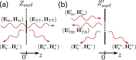
Figure 1: (Color online) Two problems for Babinet’s principle

In the first problem [problem (a)], an incident electromagnetic wave $(\mathbf{E}_{\mbox{\scriptsize\rm in}},\mathbf{H}_{\mbox{\scriptsize\rm in}})$ is scattered by the metasurface with a surface impedance $Z_{\mbox{\scriptsize\rm surf}}$ on the surface $z=0$ [see Fig. 1(a)]. Note that $Z_{\mbox{\scriptsize\rm surf}}$ is a function of $(x,y)$, but we omit the parameters for simplicity. The incident wave radiates from the sources in $z\leq 0$. If there was no metasurface, the source would produce $(\mathbf{E}_{\mbox{\scriptsize\rm in}},\mathbf{H}_{\mbox{\scriptsize\rm in}})$ in $z\leq 0$ and $(\mathbf{E}_{\mbox{\scriptsize\rm TT}},\mathbf{H}_{\mbox{\scriptsize\rm TT}})$ in $z\geq 0$. Here, $\mathrm{TT}$ represents a totally transmitted wave. The incident wave is not restricted to plane waves and can even include near-field components. If there is a metasurface, surface currents and charges are induced by the incident wave. They radiate the following scattered fields: $(\mathbf{E}^{-}_{\mbox{\scriptsize\rm s}},\mathbf{H}^{-}_{\mbox{\scriptsize\rm s}})$ in $z\leq 0$ and $(\mathbf{E}^{+}_{\mbox{\scriptsize\rm s}},\mathbf{H}^{+}_{\mbox{\scriptsize\rm s}})$ in $z\geq 0$.

Next, we set up the second problem [problem (b)]. In this problem, an incident wave $(\mathbf{E}_{\mbox{\scriptsize\rm in}}^{\prime},\mathbf{H}_{\mbox{\scriptsize\rm in}}^{\prime})$ from sources in $z\leq 0$ enters the metasurface at $z=0$ with a surface impedance $Z_{\mbox{\scriptsize\rm surf}}^{\prime}$ varying on $z=0$ [see Fig. 1(b)]. Here, $(\mathbf{E}_{\mbox{\scriptsize\rm in}}^{\prime},\mathbf{H}_{\mbox{\scriptsize\rm in}}^{\prime})$ is defined in $z\leq 0$. If a perfect electric conductor (PEC) sheet is placed at $z=0$, the incident wave is totally reflected. This totally reflected wave in $z\leq 0$ is represented by $(\mathbf{E}_{\mbox{\scriptsize\rm TR}}^{\prime},\mathbf{H}_{\mbox{\scriptsize\rm TR}}^{\prime})$. The effect of the metasurface that differs from the PEC sheet emerges as the remaining fields $(\mathbf{E}^{\prime\pm}_{\mbox{\scriptsize\rm s}},\mathbf{H}^{\prime\pm}_{\mbox{\scriptsize\rm s}})$, where $-$ and $+$ represent the fields in $z\leq 0$ and $z\geq 0$, respectively.

In general, these two problems are completely distinct. If we assume a specific condition for the surface impedances, the scattering fields of the two problems are related as described in the following theorem.

Theorem 1.

If $Z_{\mbox{\scriptsize\rm surf}}$ and $Z_{\mbox{\scriptsize\rm surf}}^{\prime}$ satisfy $Z_{\mbox{\scriptsize\rm surf}}\,Z^{\prime}_{\mbox{\scriptsize\rm surf}}=\left(Z_{0}/2\right)^{2}$ at any point with $z=0$, the scattering fields of problem (b) are given by $(\mathbf{E}^{\prime\pm}_{\mbox{\scriptsize\rm s}},\mathbf{H}^{\prime\pm}_{\mbox{\scriptsize\rm s}})=\mathcal{R}_{\pm\pi/2}(\mathbf{E}^{\pm}_{\mbox{\scriptsize\rm s}},\mathbf{H}^{\pm}_{\mbox{\scriptsize\rm s}})=\pm(Z_{0}\mathbf{H}^{\pm}_{\mbox{\scriptsize\rm s}},-\mathbf{E}^{\pm}_{\mbox{\scriptsize\rm s}}/Z_{0})$ for the incident wave $(\mathbf{E}_{\mbox{\scriptsize\rm in}}^{\prime},\mathbf{H}_{\mbox{\scriptsize\rm in}}^{\prime})=\mathcal{R}_{-\pi/2}(\mathbf{E}_{\mbox{\scriptsize\rm in}},\mathbf{H}_{\mbox{\scriptsize\rm in}})=(-Z_{0}\mathbf{H}_{\mbox{\scriptsize\rm in}},\mathbf{E}_{\mbox{\scriptsize\rm in}}/Z_{0})$ using the solution of problem (a).

Proof.

Here, we define a unit vector $\mathbf{e}_{z}$ parallel to the $z$ axis, and the projection operator $\mathcal{P}=-\mathbf{e}_{z}\times\mathbf{e}_{z}\times$, which eliminates $z$-components of vectors. First, we consider problem (a). The scattered fields $(\mathbf{E}^{\pm}_{\mbox{\scriptsize\rm s}},\mathbf{H}^{\pm}_{\mbox{\scriptsize\rm s}})$ are symmetric with respect to $z=0$. Then, $\mathcal{P}\mathbf{E}_{\mbox{\scriptsize\rm s}}^{+}=\mathcal{P}\mathbf{E}_{\mbox{\scriptsize\rm s}}^{-}$ and $\mathcal{P}\mathbf{H}_{\mbox{\scriptsize\rm s}}^{+}=-\mathcal{P}\mathbf{H}_{\mbox{\scriptsize\rm s}}^{-}$ are satisfied on $z=0$. The electric boundary condition $\mathcal{P}(\mathbf{E}_{\mbox{\scriptsize\rm TT}}+\mathbf{E}^{+}_{\mbox{\scriptsize\rm s}})=\mathcal{P}(\mathbf{E}_{\mbox{\scriptsize\rm in}}+\mathbf{E}^{-}_{\mbox{\scriptsize\rm s}})$ on $z=0$ is automatically satisfied. Another boundary condition on $z=0$ is given by $\mathcal{P}(\mathbf{E}_{\mbox{\scriptsize\rm in}}+\mathbf{E}^{-}_{\mbox{\scriptsize\rm s}})=Z_{\mbox{\scriptsize\rm surf}}\,{\mathbf{e}_{z}}\times(\mathbf{H}^{+}_{\mbox{\scriptsize\rm s}}-\mathbf{H}^{-}_{\mbox{\scriptsize\rm s}})$. With $\mathcal{P}\mathbf{H}^{+}_{\mbox{\scriptsize\rm s}}=-\mathcal{P}\mathbf{H}^{-}_{\mbox{\scriptsize\rm s}}$, we obtain the following equation for $z=0$:

$$\mathcal{P}(\mathbf{E}_{\mbox{\scriptsize\rm in}}+\mathbf{E}^{-}_{\mbox{\scriptsize\rm s}})=2Z_{\mbox{\scriptsize\rm surf}}\,{\mathbf{e}_{z}}\times\mathbf{H}^{+}_{\mbox{\scriptsize\rm s}}.$$ (4)

In problem (b), we show that the fields $(\mathbf{E}^{\prime\pm}_{\mbox{\scriptsize\rm s}},\mathbf{H}^{\prime\pm}_{\mbox{\scriptsize\rm s}})$ defined by $\mathcal{R}_{\pm\pi/2}(\mathbf{E}^{\pm}_{\mbox{\scriptsize\rm s}},\mathbf{H}^{\pm}_{\mbox{\scriptsize\rm s}})$ satisfy all boundary conditions for the incident wave $(\mathbf{E}_{\mbox{\scriptsize\rm in}}^{\prime},\mathbf{H}_{\mbox{\scriptsize\rm in}}^{\prime})=\mathcal{R}_{-\pi/2}(\mathbf{E}_{\mbox{\scriptsize\rm in}},\mathbf{H}_{\mbox{\scriptsize\rm in}})$. The fields $(\mathbf{E}^{\prime\pm}_{\mbox{\scriptsize\rm s}},\mathbf{H}^{\prime\pm}_{\mbox{\scriptsize\rm s}})=\pm(Z_{0}\mathbf{H}^{\pm}_{\mbox{\scriptsize\rm s}},-\mathbf{E}^{\pm}_{\mbox{\scriptsize\rm s}}/Z_{0})$ are also symmetric with respect to $z=0$. From $\mathcal{P}\mathbf{E}^{\prime}_{\mbox{\scriptsize\rm in}}=-\mathcal{P}\mathbf{E}^{\prime}_{\mbox{\scriptsize\rm TR}}$ and $\mathcal{P}\mathbf{E}^{\prime-}_{\mbox{\scriptsize\rm s}}=\mathcal{P}\mathbf{E}^{\prime+}_{\mbox{\scriptsize\rm s}}$ on $z=0$, the electric boundary condition $\mathcal{P}(\mathbf{E}^{\prime}_{\mbox{\scriptsize\rm in}}+\mathbf{E}^{\prime}_{\mbox{\scriptsize\rm TR}}+\mathbf{E}^{\prime-}_{\mbox{\scriptsize\rm s}})=\mathcal{P}\mathbf{E}^{\prime+}_{\mbox{\scriptsize\rm s}}$ is satisfied. Additionally, the following boundary condition should be satisfied on $z=0$:

$$\mathcal{P}\mathbf{E}^{\prime+}_{\mbox{\scriptsize\rm s}} =Z_{\mbox{\scriptsize\rm surf}}^{\prime}\,{\mathbf{e}_{z}}\times(\mathbf{H}^{\prime+}_{\mbox{\scriptsize\rm s}}-\mathbf{H}^{\prime-}_{\mbox{\scriptsize\rm s}}-\mathbf{H}^{\prime}_{\mbox{\scriptsize\rm in}}-\mathbf{H}^{\prime}_{\mbox{\scriptsize\rm TR}})$$

$$=-2Z_{\mbox{\scriptsize\rm surf}}^{\prime}\,{\mathbf{e}_{z}}\times(\mathbf{H}_{\mbox{\scriptsize\rm in}}^{\prime}+\mathbf{H}^{\prime-}_{\mbox{\scriptsize\rm s}}),$$ (5)

where we use $\mathcal{P}\mathbf{H}^{\prime+}_{\mbox{\scriptsize\rm s}}=-\mathcal{P}\mathbf{H}^{\prime-}_{\mbox{\scriptsize\rm s}}$ and $\mathcal{P}\mathbf{H}^{\prime}_{\mbox{\scriptsize\rm in}}=\mathcal{P}\mathbf{H}^{\prime}_{\mbox{\scriptsize\rm TR}}$ on $z=0$ (the derivation of $\mathcal{P}\mathbf{H}^{\prime}_{\mbox{\scriptsize\rm in}}=\mathcal{P}\mathbf{H}^{\prime}_{\mbox{\scriptsize\rm TR}}$ is shown in Appendix A). Operating with $\mathbf{e}_{z}\times$ on Eq. (5) and comparing with Eq. (4), we have $Z_{\mbox{\scriptsize\rm surf}}\,Z_{\mbox{\scriptsize\rm surf}}^{\prime}=\left(Z_{0}/2\right)^{2}$. Thus all boundary conditions are satisfied for problem (b) with $Z_{\mbox{\scriptsize\rm surf}}^{\prime}={Z_{0}}^{2}/(4Z_{\mbox{\scriptsize\rm surf}})$. ∎

For the case of $Z_{\mbox{\scriptsize\rm surf}}=\infty$ (hole), the complementary surface is PEC with $Z_{\mbox{\scriptsize\rm surf}}^{\prime}=0$, and vice versa. Therefore, the above theorem includes the standard Babinet’s principle. The extensions for tensor impedancesBaum and Singaraju (1974) and lumped elementsMoore (1993) have also been investigated.

Next, we discuss the relationship of the transmission and reflection coefficients in problems (a) and (b). From here on, we assume that all fields oscillate sinusoidally with angular frequency $\omega$ and are represented by complex amplitudes. We consider a periodic metasurface with lattice vectors $\mathbf{a}_{1}$ and $\mathbf{a}_{2}$. Physically, a metasurface without periodicity can be regarded as $|\mathbf{a}_{1}|,\ |\mathbf{a}_{2}|\rightarrow\infty$. This corresponds to the transition from box quantization to free space quantization in quantum mechanics. The reciprocal vectors are represented by $\mathbf{b}_{1}$ and $\mathbf{b}_{2}$ satisfying $\mathbf{a}_{i}\cdot\mathbf{b}_{j}=2\pi\delta_{ij}$ ($\delta_{ij}$ is the Kronecker delta). Additionally, we assume that the incident wave is a plane wave $(\tilde{\mathbf{E}}_{\mbox{\scriptsize\rm in}},\tilde{\mathbf{H}}_{\mbox{\scriptsize\rm in}})=(\check{\mathbf{E}}_{0}{\mathrm{e}}^{{\mathrm{i}}\mathbf{k}_{0}\cdot\mathbf{x}},\check{\mathbf{H}}_{0}{\mathrm{e}}^{{\mathrm{i}}\mathbf{k}_{0}\cdot\mathbf{x}})$ with $\check{{\mathbf{H}}}_{0}={Z_{0}}^{-1}\mathbf{k}_{0}\times\check{\mathbf{E}}_{0}/|\mathbf{k}_{0}|$ for a wave vector $\mathbf{k}_{0}$. Here we use the checkmark symbol in order to express complex amplitudes for a plane wave with a definite wave vector.

In problem (a), the scattered wave $(\tilde{\mathbf{E}}^{+}_{\mbox{\scriptsize\rm s}},\tilde{\mathbf{H}}^{+}_{\mbox{\scriptsize\rm s}})$ on $z=0$ has Fourier components with the in-plane wave vector $\underline{\mathbf{k}}_{pq}:=p\mathbf{b}_{1}+q\mathbf{b}_{2}+\mathcal{P}\mathbf{k}_{0}$ for $(p,q)\in\mathbb{Z}^{2}$. In this paper, we focus on the 0th-order modes with $(p,q)=(0,0)$ in order to simplify the notation. The general case is summarized in Appendix B. We decompose the 0th-order complex fields of problem (a) in $z\geq 0$ as $\sum_{\alpha=1,2}t_{\alpha}(\tilde{\mathbf{E}}^{+}_{\alpha},\tilde{\mathbf{H}}^{+}_{\alpha})$ with complex transmission coefficients $t_{\alpha}$, where we define $(\tilde{\mathbf{E}}^{+}_{1},\tilde{\mathbf{H}}^{+}_{1}):=(\tilde{\mathbf{E}}_{\mathrm{TT}},\tilde{\mathbf{H}}_{\mathrm{TT}})$, and its perpendicular polarization state $(\tilde{\mathbf{E}}^{+}_{2},\tilde{\mathbf{H}}^{+}_{2})$. The mode $(\tilde{\mathbf{E}}^{+}_{2},\tilde{\mathbf{H}}^{+}_{2})$ is normalized to carry the same power flow of $(\tilde{\mathbf{E}}^{+}_{1},\tilde{\mathbf{H}}^{+}_{1})$. We also define $(\tilde{\mathbf{E}}^{-}_{\alpha},\tilde{\mathbf{H}}^{-}_{\alpha})$ as the mirror symmetric field of $(\tilde{\mathbf{E}}^{+}_{\alpha},\tilde{\mathbf{H}}^{+}_{\alpha})$ with respect to $z=0$. In $z\leq 0$, the 0th-order field is represented by $(\tilde{\mathbf{E}}_{\mbox{\scriptsize\rm in}},\tilde{\mathbf{H}}_{\mbox{\scriptsize\rm in}})+\sum_{\alpha=1,2}r_{\alpha}(\tilde{\mathbf{E}}^{-}_{\alpha},\tilde{\mathbf{H}}^{-}_{\alpha})$ with complex reflection coefficients $r_{\alpha}$. For problem (b), we define $(\tilde{\mathbf{E}}^{\prime\pm}_{\alpha},\tilde{\mathbf{H}}^{\prime\pm}_{\alpha}):=\mathcal{R}_{\mp\pi/2}(\tilde{\mathbf{E}}^{\pm}_{\alpha},\tilde{\mathbf{H}}^{\pm}_{\alpha})$. The 0th-order fields are written as $\sum_{\alpha=1,2}t^{\prime}_{\alpha}(\tilde{\mathbf{E}}^{\prime+}_{\alpha},\tilde{\mathbf{H}}^{\prime+}_{\alpha})$ in $z\geq 0$, and $(\tilde{\mathbf{E}}^{\prime}_{\mbox{\scriptsize\rm in}},\tilde{\mathbf{H}}^{\prime}_{\mbox{\scriptsize\rm in}})+\sum_{\alpha=1,2}r^{\prime}_{\alpha}(\tilde{\mathbf{E}}^{\prime-}_{\alpha},\tilde{\mathbf{H}}^{\prime-}_{\alpha})$ in $z\leq 0$.

Now we formulate Babinet’s principle for complex coefficients as follows:

Theorem 2.

The coefficients of the two problems are related as $t_{1}+t_{1}^{\prime}=1$, $r_{1}+r^{\prime}_{1}=-1$, and $t_{2}+t^{\prime}_{2}=0$, $r_{2}+r^{\prime}_{2}=0$.

Proof.

For problem (a), the 0th-order component of the scattered field in $z\geq 0$ is given by

$$(\tilde{\mathbf{E}}^{+}_{\mbox{\scriptsize\rm s0}},\tilde{\mathbf{H}}^{+}_{\mbox{\scriptsize\rm s0}})=-(\tilde{\mathbf{E}}^{+}_{1},\tilde{\mathbf{H}}^{+}_{1})+\sum_{\alpha=1,2}t_{\alpha}(\tilde{\mathbf{E}}^{+}_{\alpha},\tilde{\mathbf{H}}^{+}_{\alpha}).$$ (6)

In problem (b), the 0th-order component of $(\tilde{\mathbf{E}}^{\prime+}_{\mbox{\scriptsize\rm s}},\tilde{\mathbf{H}}^{\prime+}_{\mbox{\scriptsize\rm s}})$ is

$$(\tilde{\mathbf{E}}^{\prime+}_{\mbox{\scriptsize\rm s0}},\tilde{\mathbf{H}}^{\prime+}_{\mbox{\scriptsize\rm s0}})=\sum_{\alpha=1,2}t^{\prime}_{\alpha}(\tilde{\mathbf{E}}^{\prime+}_{\alpha},\tilde{\mathbf{H}}^{\prime+}_{\alpha}).$$ (7)

Applying $\mathcal{R}_{-\pi/2}$ to Eq. (7), we have

$$(\tilde{\mathbf{E}}^{+}_{\mbox{\scriptsize\rm s0}},\tilde{\mathbf{H}}^{+}_{\mbox{\scriptsize\rm s0}})=-\sum_{\alpha=1,2}t^{\prime}_{\alpha}(\tilde{\mathbf{E}}^{+}_{\alpha},\tilde{\mathbf{H}}^{+}_{\alpha}),$$ (8)

where we use $(\mathbf{E}^{\prime+}_{\mbox{\scriptsize\rm s0}},\mathbf{H}^{\prime+}_{\mbox{\scriptsize\rm s0}})=\mathcal{R}_{\pi/2}(\mathbf{E}^{+}_{\mbox{\scriptsize\rm s0}},\mathbf{H}^{+}_{\mbox{\scriptsize\rm s0}})$ and $(\mathbf{E}^{\prime+}_{\alpha},\mathbf{H}^{\prime+}_{\alpha})=\mathcal{R}_{-\pi/2}(\mathbf{E}^{+}_{\alpha},\mathbf{H}^{+}_{\alpha})$. Comparing Eq. (8) with Eq. (6), we obtain $t_{1}+t_{1}^{\prime}=1$ and $t_{2}+t_{2}^{\prime}=0$. The remaining equations are derived from a similar discussion for $z\leq 0$. ∎

IV Self-complementary metasurfaces

For a metasurface with a surface impedance $Z_{\mbox{\scriptsize\rm surf}}$, we can create the complementary metasurface with $Z_{\mbox{\scriptsize\rm surf}}^{\prime}={Z_{0}}^{2}/(4Z_{\mbox{\scriptsize\rm surf}})$. This operation is called an impedance inversion about $Z_{0}/2$. Two metasurfaces are congruent if one can be transformed into the other by a combination of translations, rotations and reflections. When a metasurface is congruent to its complementary one, we say that it is self-complementary. We emphasize that the self-complementarity is not the same as the point-group symmetry. Several examples of self-complementary metasurfaces are shown in Fig. 2.

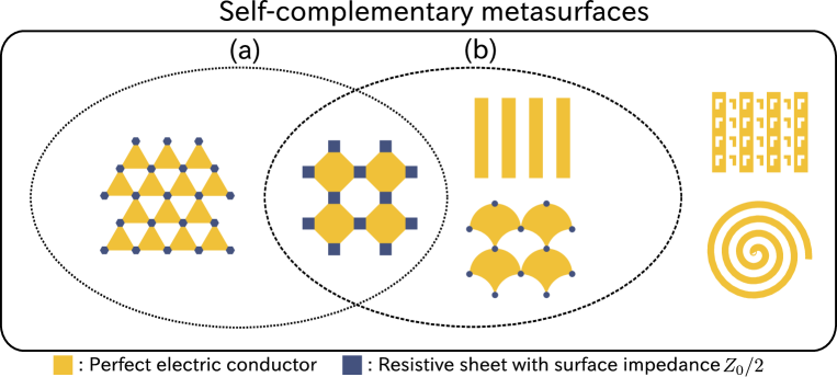
Figure 2: (Color online) Examples of self-complementary metasurfaces. The class of self-complementary metasurfaces includes two specific subclasses with (a) $n$-fold rotational symmetry ($n\geq 3$) and (b) translational self-complementarity.

For a left circularly polarized incident wave, we define $t_{\mbox{\scriptsize\rm LL}}:=t_{1}$, $t_{\mbox{\scriptsize\rm RL}}:=t_{2}$, and $r_{\mbox{\scriptsize\rm RL}}:=r_{1}$, $r_{\mbox{\scriptsize\rm LL}}:=r_{2}$. We also use $t_{\mbox{\scriptsize\rm RR}}:=t_{1}$, $t_{\mbox{\scriptsize\rm LR}}:=t_{2}$, and $r_{\mbox{\scriptsize\rm LR}}:=r_{1}$, $r_{\mbox{\scriptsize\rm RR}}:=r_{2}$ for a right circularly polarized incident wave. From reciprocity and the mirror symmetry of a metasurface with respect to $z=0$, the following theorem is derived.

Theorem 3.

In the case of normal incidence of a circularly polarized plane wave onto a metasurface, $t_{\mbox{\scriptsize\rm RR}}=t_{\mbox{\scriptsize\rm LL}}$ and $r_{\mbox{\scriptsize\rm LR}}=r_{\mbox{\scriptsize\rm RL}}$ are satisfied.

Proof.

We consider two situations. In the first, the incident wave is a left circularly polarized wave $(\tilde{\mathbf{E}}_{\mbox{\scriptsize\rm in}},\tilde{\mathbf{H}}_{\mbox{\scriptsize\rm in}})=(\check{E}_{0}\mathbf{e}_{+},-{\mathrm{i}}\check{H}_{0}\mathbf{e}_{+}){\mathrm{e}}^{{\mathrm{i}}k_{0}z}$ from $z\leq 0$, where $\check{H}_{0}=\check{E}_{0}/Z_{0}$ and $\mathbf{e}_{\pm}:=(\mathbf{e}_{x}\pm{\mathrm{i}}\mathbf{e}_{y})/\sqrt{2}$ with unit vectors $\mathbf{e}_{x}$ and $\mathbf{e}_{y}$ along $x$ and $y$ axes. The total field is represented by $(\tilde{\mathbf{E}}_{\mbox{\scriptsize\rm f}},\tilde{\mathbf{H}}_{\mbox{\scriptsize\rm f}})$. In the second situation, an incident wave from $z\geq 0$ is $(\tilde{\mathbf{E}}_{\mbox{\scriptsize\rm in}},\tilde{\mathbf{H}}_{\mbox{\scriptsize\rm in}})=(\check{E}_{0}\mathbf{e}_{-},{\mathrm{i}}\check{H}_{0}\mathbf{e}_{-}){\mathrm{e}}^{-{\mathrm{i}}k_{0}z}$, and the total field is denoted by $(\tilde{\mathbf{E}}_{\mbox{\scriptsize\rm b}},\tilde{\mathbf{H}}_{\mbox{\scriptsize\rm b}})$. If we perform the coordinate transformation $z\rightarrow-z$, the second situation can be transformed to the scattering problem for a right circularly polarized incident wave from $z\leq 0$, because of the symmetry between the front and back of the metasurface. Then, $t_{1}$ of the second situation is equivalent to $t_{\mbox{\scriptsize\rm RR}}$.

We represent the unit cell on $z=0$ by $U$, and consider $V=U\times[h/2,h/2]$ with $h>0$. For the normal incidence, we can impose periodic boundary conditions on two pairs of opposite faces of $\partial U\times[h/2,h/2]$. From the Lorentz reciprocity theoremCollin (1991)

$$\int_{\partial V}(\tilde{\mathbf{E}}_{\mbox{\scriptsize\rm f}}\times\tilde{\mathbf{H}}_{\mbox{\scriptsize\rm b}}-\tilde{\mathbf{E}}_{\mbox{\scriptsize\rm b}}\times\tilde{\mathbf{H}}_{\mbox{\scriptsize\rm f}})\cdot{\mathrm{d}}\mathbf{S}=0$$ (9)

and $\mathbf{e}_{+}\times\mathbf{e}_{-}=-{\mathrm{i}}\mathbf{e}_{\mbox{\scriptsize\rm z}}$, we obtain $t_{\mbox{\scriptsize\rm RR}}=t_{\mbox{\scriptsize\rm LL}}$. Because electric fields are continuous on $z=0$, $1+r_{\mbox{\scriptsize\rm LR}}=t_{\mbox{\scriptsize\rm RR}}$ and $1+r_{\mbox{\scriptsize\rm RL}}=t_{\mbox{\scriptsize\rm LL}}$ are satisfied. Then, $r_{\mbox{\scriptsize\rm LR}}=r_{\mbox{\scriptsize\rm RL}}$ is proved. ∎

By using Theorems 2 and 3, we can arrive at the following theorem.

Theorem 4.

In the case of normal incidence of a circularly polarized plane wave onto a self-complementary metasurface, $t_{\mbox{\scriptsize\rm RR}}=t_{\mbox{\scriptsize\rm LL}}=1/2$ and $r_{\mbox{\scriptsize\rm LR}}=r_{\mbox{\scriptsize\rm RL}}=-1/2$ are satisfied.

Proof.

This situation is regarded as problem (a) shown in Fig. 1. Because the metasurface is self-complementary, its complement returns to the original metasurface by the finite numbers of reflections. The product of these operations is denoted by $\mathcal{X}$. Problem (b) related to problem (a) through Theorem 1 is considered. Applying $\mathcal{X}$ to all fields and structures of problem (b), we have problem (c). Now, we consider the two cases where even and odd numbers of the reflections are involved in $\mathcal{X}$. In the even case, $(\tilde{\mathbf{E}}_{\mbox{\scriptsize\rm in}},\tilde{\mathbf{H}}_{\mbox{\scriptsize\rm in}})$ is an eigenmode for $\mathcal{X}$. Therefore, problem (c) is identical to problem (a) except for the total phase, and $t^{\prime}_{1}=t_{1}$ is satisfied, where the transmission coefficient $t^{\prime}_{1}$ of problem (b) is defined in Sec. III. In the case of odd reflections, the polarization is changed by $\mathcal{X}$ (for example, from LCP to RCP), but Theorem 3 assures $t^{\prime}_{1}=t_{1}$. Finally, we obtain $t^{\prime}_{1}=t_{1}=1/2$ from Theorem 2 for both cases. ∎

We note that the frequency-independent transmission of self-complementary metasurfaces is valid in the high-frequency range with diffraction. In the following, we consider subclasses of self-complementary metasurfaces shown in Fig. 2.

If a metasurface has rotational symmetry in addition to self-complementarity [see Fig. 2(a)], we have the following theorem.

Theorem 5.

For normal incidence of a plane wave with an arbitrary polarization onto a self-complementary metasurface with $n$-fold rotational symmetry $(n\geq 3)$, $t_{1}=1/2$, $r_{1}=-1/2$ and $t_{2}=0$, $r_{2}=0$ are satisfied. Half the incident power is absorbed by the metasurface in the frequency range without diffraction.

Proof.

We consider two incident waves in $z\leq 0$: $(\tilde{\mathbf{E}}^{\mbox{\scriptsize\rm L}}_{\mbox{\scriptsize\rm in}},\tilde{\mathbf{H}}_{\mbox{\scriptsize\rm in}}^{\mbox{\scriptsize\rm L}})=(\check{E}_{0}\mathbf{e}_{+},-{\mathrm{i}}\check{H}_{0}\mathbf{e}_{+}){\mathrm{e}}^{{\mathrm{i}}k_{0}z}$ and $(\tilde{\mathbf{E}}_{\mbox{\scriptsize\rm in}}^{\mbox{\scriptsize\rm R}},\tilde{\mathbf{H}}_{\mbox{\scriptsize\rm in}}^{\mbox{\scriptsize\rm R}})=(\check{E}_{0}\mathbf{e}_{-},{\mathrm{i}}\check{H}_{0}\mathbf{e}_{-}){\mathrm{e}}^{{\mathrm{i}}k_{0}z}$. Here, we define $(\tilde{\mathbf{E}}_{\alpha}^{+,\beta},\tilde{\mathbf{H}}_{\alpha}^{+,\beta})$ as $(\tilde{\mathbf{E}}_{\alpha}^{\mbox{\scriptsize\rm+}},\tilde{\mathbf{H}}_{\alpha}^{\mbox{\scriptsize\rm+}})$ for an incident wave with polarization $\beta$. We adjust the phase of $(\tilde{\mathbf{E}}_{2}^{\mbox{\scriptsize\rm+}},\tilde{\mathbf{H}}_{2}^{\mbox{\scriptsize\rm+}})$ so as to satisfy $(\tilde{\mathbf{E}}_{2}^{\mbox{\scriptsize\rm+,R}},\tilde{\mathbf{H}}_{2}^{\mbox{\scriptsize\rm+,R}})=(\tilde{\mathbf{E}}_{1}^{\mbox{\scriptsize\rm+,L}},\tilde{\mathbf{H}}_{1}^{\mbox{\scriptsize\rm+,L}})$ and $(\tilde{\mathbf{E}}_{2}^{\mbox{\scriptsize\rm+,L}},\tilde{\mathbf{H}}_{2}^{\mbox{\scriptsize\rm+,L}})=(\tilde{\mathbf{E}}_{1}^{\mbox{\scriptsize\rm+,R}},\tilde{\mathbf{H}}_{1}^{\mbox{\scriptsize\rm+,R}})$ on $z=0$, for each incident wave. In this situation, we can define a complex transmittance matrix

$$\tau=\begin{bmatrix}t_{\mbox{\scriptsize\rm LL}}&t_{\mbox{\scriptsize\rm LR}}\\ t_{\mbox{\scriptsize\rm RL}}&t_{\mbox{\scriptsize\rm RR}}\end{bmatrix}.$$ (10)

For a circularly polarized basis, a rotation by $2\pi/n$ about $z$ axis is represented by

$$P:=\begin{bmatrix}{\mathrm{e}}^{-{\mathrm{i}}\frac{2\pi}{n}}&0\\ 0&{\mathrm{e}}^{{\mathrm{i}}\frac{2\pi}{n}}\end{bmatrix}.$$ (11)

Because of $n$-fold symmetry, $P^{-1}\tau P=\tau$ is satisfied, and then $t_{\mbox{\scriptsize\rm RL}}=t_{\mbox{\scriptsize\rm LR}}=0$. Therefore, we obtain

$$\tau=\begin{bmatrix}\frac{1}{2}&0\\ 0&\frac{1}{2}\end{bmatrix},$$ (12)

from Theorem 4. Because $\tau$ is proportional to the identity matrix, $t_{1}=1/2$, $r_{1}=-1/2$ and $t_{2}=0$, $r_{2}=0$ are satisfied for an incident plane wave with an arbitrary polarization.

In the frequency range without diffraction, the Fourier components of $(\tilde{\mathbf{E}}^{\pm}_{\mbox{\scriptsize\rm s}},\tilde{\mathbf{H}}^{\pm}_{\mbox{\scriptsize\rm s}})$ with $(p,q)\neq 0$ are evanescent waves. For evanescent waves, the real part of the $z$-component of Poyinting vectors is zero; therefore, they do not carry energy out of $z=0$. The remaining power $A=1-|t_{1}|^{2}-|r_{1}|^{2}=1/2$ is absorbed in the metasurface. ∎

From Theorem 5, we find that the metasurface can absorb total incident energy as follows:

Theorem 6.

If we excite a self-complementary metasurface with $n$-fold rotational symmetry $(n\geq 3)$ by two in-phase plane waves $(\check{\mathbf{E}}_{0},\check{\mathbf{H}}_{0}){\mathrm{e}}^{{\mathrm{i}}k_{0}z}$ from $z\leq 0$ and $(\check{\mathbf{E}}_{0},-\check{\mathbf{H}}_{0}){\mathrm{e}}^{-{\mathrm{i}}k_{0}z}$ from $z\geq 0$ with an arbitrary polarization $(\check{\mathbf{E}}_{0},\check{\mathbf{H}}_{0})$, the incident power is perfectly absorbed in the frequency range without diffraction.

Proof.

In the case of one excitation $(\check{\mathbf{E}}_{0},\check{\mathbf{H}}_{0}){\mathrm{e}}^{{\mathrm{i}}k_{0}z}$ from $z\leq 0$, half of the power is absorbed in the frequency range without diffraction. If we excite from both sides in phase, the electric field is doubled, and then absorption is quadrupled. Therefore, all of the incident power is absorbed. ∎

If we excite the above self-complementary metasurface by two antiphase plane waves, there is no absorption. This is because boundary conditions at $z=0$ are already satisfied without induced currents and charges. The perfect absorption is only realized when two beams have the correct relative phase and amplitude. This function is referred to as coherent perfect absorption.Chong et al. (2010); Wan et al. (2011) We note that self-complementarity is not a necessary condition for the frequency-independent response described in Theorem 7 because a similar frequency-independent response can be seen in other systems, such as percolated metallic filmsYagil and Deutscher (1987, 1988); Gadenne et al. (1988, 1989); Beghdadi et al. (1989); Davis et al. (1991); Sarychev et al. (1995) and two identical lamellar gratings.Botten et al. (1997)

There is another interesting class of self-complementary metasurfaces. If a metasurface returns to the original one by just a translation after the impedance inversion about $Z_{0}/2$, we say that it has translational self-complementarity [see Fig. 2(b)]. This subclass of self-complementary metasurfaces has the following property.

Theorem 7.

In the case of an oblique incidence of a circularly polarized plane wave onto a metasurface with translational self-complementarity, $t_{\mbox{\scriptsize\rm RR}}=t_{\mbox{\scriptsize\rm LL}}=1/2$ and $r_{\mbox{\scriptsize\rm LR}}=r_{\mbox{\scriptsize\rm RL}}=-1/2$ are satisfied.

Proof.

We regard this situation as problem (a) shown in Fig. 1. The metasurface returns to the original position by a translation $\mathcal{T}$ together with the impedance inversion. Problem (b) can be related to problem (a) through Theorem 1. We introduce problem (c) in which the incident wave and the metasurface of problem (b) are translated by $\mathcal{T}$. From the definition of $\mathcal{T}$, the metasurface of problem (c) is the same as that in problem (a). The incident field of problem (c) is written as $\mathcal{T}\mathcal{R}_{-\pi/2}(\tilde{\mathbf{E}}_{\mbox{\scriptsize\rm in}},\tilde{\mathbf{H}}_{\mbox{\scriptsize\rm in}})$. Because $(\tilde{\mathbf{E}}_{\mbox{\scriptsize\rm in}},\tilde{\mathbf{H}}_{\mbox{\scriptsize\rm in}})$ is an eigenmode for $\mathcal{T}\mathcal{R}_{-\pi/2}$, the incident wave of problem (c) is identical to that of problem (a) except for the total phase. In this way, $t^{\prime}_{1}=t_{1}$ and $r^{\prime}_{1}=r_{1}$ are confirmed. From Theorem 2, we have $t^{\prime}_{1}=t_{1}=1/2$ and $r^{\prime}_{1}=r_{1}=-1/2$. ∎

This theorem shows that self-complementary metasurfaces can be used as beam splitters. The extension for general diffraction orders is discussed in Appendix C.

V Examples: checkerboard metasurfaces

In this section, we apply the current theory for checkerboard metasurfacesCompton et al. (1984); Takano et al. ; Edmunds et al. (2010); Kempa (2010); Ramakrishna et al. (2011) and confirm its validity by simulations. First, we consider an ideal checkerboard metasurface shown in Fig. 3(a). It is expected that the ideal checkerboard metasurface should exhibit a frequency-independent response because of its self-complementarity. However, it is known that the ideal checkerboard metasurface cannot be realized. This is explained as follows.Takano et al. The electromagnetic response of the checkerboard metasurface drastically changes depending on whether the square metals are connected or not. The transmittance and reflectance do not converge when the structure approaches the ideal checkerboard metasurface. Furthermore, it has also been reported that there is an instability in numerical calculations for the ideal checkerboard metasurface, and the checkerboard metasurfaces exhibit percolation effects near the ideal checkerboard metasurface.Kempa (2010)

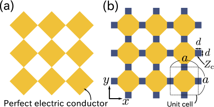
Figure 3: (Color online) (a) Ideal checkerboard metasurface (b) Resistive checkerboard metasurface

By using our theory, we can give another explanation without relying on asymptotic behaviors. From Theorem 5, the power transmission $T=|t_{1}|^{2}$ and reflection $R=|r_{1}|^{2}$ should satisfy $T=R=1/4$ for the ideal checkerboard metasurface with 4-fold rotational symmetry. However, energy conservation means $T+R=1$ in the frequency range without diffraction, because there is no absorption in the perfect checkerboard metasurface. This contradiction implies that the ideal checkerboard metasurface is unphysical.

The above explanation gives us another insight: we may realize the frequency-independent response of a checkerboard metasurface if resistive elements are introduced. We replace the singular contacts with tiny resistive sheets with a surface impedance $Z_{\mbox{\scriptsize\rm c}}$ and obtain a resistive checkerboard metasurface shown in Fig. 3(b). When $Z_{\mbox{\scriptsize\rm c}}=Z_{0}/2$ is satisfied, the resistive checkerboard metasurface is self-complementary and is expected to exhibit a frequency-independent response.

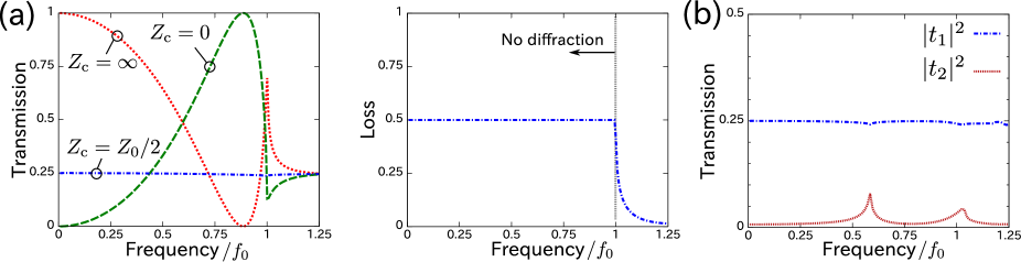
Figure 4: (Color online) (a) Power transmission and loss spectra for normally incident $x$-polarized plane waves entering into resistive checkerboard metasurfaces with $d/a=0.2$. The left graph shows power transmission spectra for resistive checkerboard metasurfaces with $Z_{\mbox{\scriptsize\rm c}}=0,\,Z_{0}/2$, and $\infty$. The right graph shows the loss spectrum calculated for the self-complementary resistive checkerboard metasurface with $Z_{\mbox{\scriptsize\rm c}}=Z_{0}/2$. (b) The calculated spectra of $|t_{1}|^{2}$ and $|t_{2}|^{2}$ for an oblique incident circularly polarized plane wave entering into the resistive checkerboard metasurfaces with $Z_{\mbox{\scriptsize\rm c}}=Z_{0}/2$ and $d/a=0.2$. The incident wave has a wave vector $\mathbf{k}_{0}=(k_{0}\sin\theta,0,k_{0}\cos\theta)$ with $\theta=\pi/4$. In these simulations, the frequencies are normalized by $f_{0}=c_{0}/a$.

For confirmation of our theory, we calculate the electromagnetic response of resistive checkerboard metasurfaces on $z=0$ by a commercial finite-element method solver (Ansoft HFSS). In the simulation, normal incident $x$-polarized plane wave is injected onto resistive checkerboard metasurfaces with $d/a=0.2$, where $a$ and $d$ are the side length of the square unit cell and that of impedance sheet, respectively. By imposing periodic boundaries on four sides, the electromagnetic fields in the unit cell are calculated for $Z_{\mbox{\scriptsize\rm c}}=0,\,Z_{0}/2$, and $\infty$. We take into account diffracted modes with $\{(p,q,\alpha)|-1\leq p\leq 1,\ -1\leq q\leq 1,\ \alpha=1,2\}$ (18 modes), where $(p,q)$ and $\alpha$ are defined in Sec. III and Appendix B.

The left panel of Fig. 4(a) displays the spectra of power transmission $|t_{1}|^{2}$ for resistive checkerboard metasurfaces with $Z_{\mbox{\scriptsize\rm c}}=0,\,Z_{0}/2$, and $\infty$. The frequency in the horizontal axis is normalized by $f_{0}:=c_{0}/a$ ($c_{0}$ is the speed of light in a vacuum). Above the frequency $f_{0}$, diffracted waves can propagate in free space. The checkerboard metasurfaces with $Z_{\mbox{\scriptsize\rm c}}=0$ and $\infty$ resonate at the same frequency $f/f_{0}=0.89$. Babinet’s principle assures that the sum of these transmission spectra equals 1 in the region of $f\leq f_{0}$, because the checkerboard metasurface with $Z_{\mbox{\scriptsize\rm c}}=\infty$ is complementary to that with $Z_{\mbox{\scriptsize\rm c}}=0$. For the resistive checkerboard metasurface with $Z_{\mbox{\scriptsize\rm c}}=Z_{0}/2$, transmission equals to $1/4$ independent of frequency, even when diffraction takes place ($f\geq f_{0}$). This constant response seems very strange, because metasurfaces made from metal usually exhibit a resonant response, but it can be explained by Theorem 5. In addition to the magnitude of transmission, we also confirm the phase of $t_{1}$. For $0<f/f_{0}\leq 1.25$, we have $|\mathop{\mathrm{Im}}[t_{1}]/\mathop{\mathrm{Re}}[t_{1}]|<1.2\times 10^{-2}$. This result shows $t_{1}=1/2$ expected by Theorem 5.

The right panel of Fig. 4(a) shows the spectrum of energy loss for the resistive checkerboard metasurface with $Z_{\mbox{\scriptsize\rm c}}=Z_{0}/2$. The loss is calculated by integration of the Poyinting vector over the resistive sheets. In the frequency range $f\leq f_{0}$, we can see that half the incident power is absorbed by the metasurface, while the electromagnetic energy is converted to diffracted modes in $f\geq f_{0}$. These results agree with Theorem 5, and coherent perfect absorption can be realized for the two-side excitations. Perfect absorption occurs for any $d/a$. The resistive checkerboard metasurface with tiny resistive sheets can absorb energy in very small regions. This property can be useful for the enhancement of non-linearity of resistance.

The resistive checkerboard metasurface with $Z_{\mbox{\scriptsize\rm c}}=Z_{0}/2$ also has translational self-complementarity. Then, it exhibits frequency-independent response for oblique incident waves. By using HFSS, we calculated the response of the resistive checkerboard metasurfaces with $Z_{\mbox{\scriptsize\rm c}}=Z_{0}/2$ for an oblique incidence of a circularly polarized plane wave with incident angle $45^{\circ}$ in the $xz$-plane. In this case, we obtain the same transmission spectra for the right and left circularly polarized incident waves. The obtained spectra of $|t_{1}|^{2}$ and $|t_{2}|^{2}$ are shown in Fig. 4(b). We can see that $|t_{1}|^{2}=1/4$, while $|t_{2}|^{2}$ has two non-zero resonant peaks at $f/f_{0}=0.58$ and $1.02$. Slight changes of $|t_{1}|^{2}$ are considered as numerical errors. For $0<f/f_{0}\leq 1.25$, we have $|\mathop{\mathrm{Im}}[t_{1}]/\mathop{\mathrm{Re}}[t_{1}]|<1.7\times 10^{-2}$. This result supports the validity of Theorem 7. The two peaks of $|t_{2}|^{2}$ are originated from the interaction between lattice sites. Periodic systems exhibit such singular behaviors when a diffracted beam grazes to the plane $z=0$ (Rayleigh condition),García de Abajo (2007) and in our system, the Rayleigh condition is satisfied at $f/f_{0}=1$ and $f/f_{0}=2-\sqrt{2}=0.586$. These frequencies correspond to the peaks shown in the graph. Then, $|t_{2}|^{2}$ shows resonant behaviors near these frequencies, while $|t_{1}|^{2}$ should be constant because of translational self-complementarity.

VI Summary

In this paper, we analyzed theoretically electromagnetic plane-wave scattering by self-complementary metasurfaces. In order to study the response of self-complementary metasurfaces, we first described the electromagnetic duality and Babinet’s principle with resistive elements. Next, by applying Babinet’s principle, we obtained the relation of scattering coefficients for a metasurface and its complement. Using this result, we revealed that the frequency-independent transmission and reflection are realized for self-complementary metasurfaces. In the case of normal incidence of a circularly polarized plane wave onto a self-complementary metasurface, complex transmission and reflection coefficients of the 0th-order diffraction must be $1/2$ and $-1/2$, respectively. If a self-complementary metasurface additionally has $n$-fold rotational symmetry $(n\geq 3)$, the above result is valid for normal incidence of a plane wave with an arbitrary polarization. Furthermore, we found that this type of metasurface acts as a coherent perfect absorber. We also studied metasurfaces with translational self-complementarity. For an oblique incidence of a circularly polarized plane wave to a metasurface with translational self-complementarity, complex transmission and reflection coefficients of the 0th diffraction order also equal to $1/2$ and $-1/2$, respectively. These results are confirmed by numerical simulations for resistive checkerboard metasurfaces.

Appendix A The relation between totally transmitted and totally reflected waves

We consider an incident wave $(\mathbf{E}_{\mbox{\scriptsize\rm in}},\mathbf{H}_{\mbox{\scriptsize\rm in}})$ in $z\leq 0$ and the totally transmitted wave $(\mathbf{E}_{\mbox{\scriptsize\rm TT}},\mathbf{H}_{\mbox{\scriptsize\rm TT}})$ in $z\geq 0$. If there is a surface made of PEC on $z=0$, the incident wave is totally reflected. This totally reflected wave is denoted by $(\mathbf{E}_{\mbox{\scriptsize\rm TR}},\mathbf{H}_{\mbox{\scriptsize\rm TR}})$. We show that $(\mathbf{E}_{\mbox{\scriptsize\rm TR}},\mathbf{H}_{\mbox{\scriptsize\rm TR}})$ can be represented by $(\mathbf{E}_{\mbox{\scriptsize\rm TT}},\mathbf{H}_{\mbox{\scriptsize\rm TT}})$ like the method of images used in electrostatics. We define $\mathcal{M}$ as the mirror reflection with respect to $z=0$. If we assume

$$(\mathbf{E}_{\mbox{\scriptsize\rm TR}},\mathbf{H}_{\mbox{\scriptsize\rm TR}})=-(\mathcal{M}\mathbf{E}_{\mbox{\scriptsize\rm TT}},\mathcal{M}\mathbf{H}_{\mbox{\scriptsize\rm TT}}),$$ (13)

the boundary condition of perfect electric conductor is satisfied. This is because $\mathcal{P}(\mathbf{E}_{\mbox{\scriptsize\rm in}}+\mathbf{E}_{\mbox{\scriptsize\rm TR}})=\mathcal{P}(\mathbf{E}_{\mbox{\scriptsize\rm in}}-\mathcal{M}\mathbf{E}_{\mbox{\scriptsize\rm TT}})=0$ for $z=0$. Then, the definition of Eq. (13) is valid. Because magnetic fields are axial vectors, $\mathcal{P}\mathcal{M}\mathbf{H}_{\mbox{\scriptsize\rm TT}}=-\mathcal{P}\mathbf{H}_{\mbox{\scriptsize\rm in}}$ is satisfied on $z=0$. From this equation and Eq. (13),

$$\mathcal{P}\mathbf{H}_{\mbox{\scriptsize\rm TR}}=\mathcal{P}\mathbf{H}_{\mbox{\scriptsize\rm in}}$$ (14)

is satisfied for $z=0$.

Appendix B Relation of scattering coefficients for all diffracted components

We generalize Theorem 2 to include all diffracted modes. The two problems discussed in Sec. III are considered. For $(p,q)=(0,0)$, we define $(\tilde{\mathbf{E}}^{+}_{pq,1},\tilde{\mathbf{H}}^{+}_{pq,1}):=(\tilde{\mathbf{E}}_{\mathrm{TT}},\tilde{\mathbf{H}}_{\mathrm{TT}})$ and its perpendicular polarization state $(\tilde{\mathbf{E}}^{+}_{pq,2},\tilde{\mathbf{H}}^{+}_{pq,2})$. For $(p,q)\neq(0,0)$, we also define $(\tilde{\mathbf{E}}^{+}_{pq,1},\tilde{\mathbf{H}}^{+}_{pq,1})$ and $(\tilde{\mathbf{E}}^{+}_{pq,2},\tilde{\mathbf{H}}^{+}_{pq,2})$ that are two orthogonal polarized modes with the factor ${\mathrm{e}}^{{\mathrm{i}}\underline{\mathbf{k}}_{pq}\cdot\mathbf{x}}{\mathrm{e}}^{{\mathrm{i}}k_{z}z}$, where $k_{z}=\sqrt{|\mathbf{k}_{0}|^{2}-|{\underline{\mathbf{k}}_{pq}}|^{2}}$ ($\mathop{\mathrm{Im}}k_{z}\geq 0$). The mirror symmetric fields of $(\tilde{\mathbf{E}}^{+}_{pq,\alpha},\tilde{\mathbf{H}}^{+}_{pq,\alpha})$ with respect to $z=0$ are denoted by $(\tilde{\mathbf{E}}^{-}_{pq,\alpha},\tilde{\mathbf{H}}^{-}_{pq,\alpha})$.

We then decompose the complex field of problem (a) in $z\geq 0$ as

$$\sum_{(p,q)\in\mathbb{Z}^{2}}\sum_{\alpha=1,2}t_{pq,\alpha}(\tilde{\mathbf{E}}^{+}_{pq,\alpha},\tilde{\mathbf{H}}^{+}_{pq,\alpha})$$

with complex transmission coefficients $t_{pq,\alpha}$. In $z\leq 0$, the field is given by

$$(\tilde{\mathbf{E}}_{\mbox{\scriptsize\rm in}},\tilde{\mathbf{H}}_{\mbox{\scriptsize\rm in}})+\sum_{(p,q)\in\mathbb{Z}^{2}}\sum_{\alpha=1,2}r_{pq,\alpha}(\tilde{\mathbf{E}}^{-}_{pq,\alpha},\tilde{\mathbf{H}}^{-}_{pq,\alpha}).$$

For problem (b), we define $(\tilde{\mathbf{E}}^{\prime\pm}_{pq,\alpha},\tilde{\mathbf{H}}^{\prime\pm}_{pq,\alpha}):=\mathcal{R}_{\mp\pi/2}(\tilde{\mathbf{E}}^{\pm}_{pq,\alpha},\tilde{\mathbf{H}}^{\pm}_{pq,\alpha})$. The fields in problem (b) are represented as follows:

$$\sum_{(p,q)\in\mathbb{Z}^{2}}\sum_{\alpha=1,2}t^{\prime}_{pq,\alpha}(\tilde{\mathbf{E}}^{\prime+}_{pq,\alpha},\tilde{\mathbf{H}}^{\prime+}_{pq,\alpha})$$

in $z\geq 0$, and

$$(\tilde{\mathbf{E}}^{\prime}_{\mbox{\scriptsize\rm in}},\tilde{\mathbf{H}}^{\prime}_{\mbox{\scriptsize\rm in}})+\sum_{(p,q)\in\mathbb{Z}^{2}}\sum_{\alpha=1,2}r^{\prime}_{pq,\alpha}(\tilde{\mathbf{E}}^{\prime-}_{pq,\alpha},\tilde{\mathbf{H}}^{\prime-}_{pq,\alpha})$$

in $z\leq 0$. Now, we can generalize Theorem 2 as follows:

Theorem 8.

$t_{00,1}+t_{00,1}^{\prime}=1$, $r_{00,1}+r^{\prime}_{00,1}=-1$, and $t_{pq,\alpha}+t^{\prime}_{pq,\alpha}=0$, $r_{pq,\alpha}+r^{\prime}_{pq,\alpha}=0$ for $(p,q,\alpha)\neq(0,0,1)$.

The proof of Theorem 8 is similar to that of Theorem 2.

Appendix C General order diffraction by metasurfaces with translational self-complementarity

We discuss the general scattering components of diffracted waves by metasurfaces with translational self-complementarity. An oblique incidence of a circularly polarized plane wave is considered. We define $W:=\{(p,q)\in\mathbb{Z}^{2};|\underline{\mathbf{k}}_{pq}|<|\mathbf{k}_{0}|\}$. For $(p,q)\in W$, the waves with the wave vector $\underline{\mathbf{k}}_{pq}\pm\sqrt{{k_{0}}^{2}-|{\underline{\mathbf{k}}_{pq}}|^{2}}\,\mathbf{e}_{z}$ are not evanescent but propagating plane waves. $(\tilde{\mathbf{E}}^{+}_{00,1},\tilde{\mathbf{H}}^{+}_{00,1})$ represents the totally transmitted plane wave with circular polarization. For $(p,q)\in W$ satisfying $(p,q)\neq(0,0)$, $(\tilde{\mathbf{E}}^{+}_{pq,1},\tilde{\mathbf{H}}^{+}_{pq,1})$ are selected to be the circularly polarized plane waves with the same helicity of $(\tilde{\mathbf{E}}^{+}_{00,1},\tilde{\mathbf{H}}^{+}_{00,1})$. Now, Theorem 7 is extended as follows:

Theorem 9.

For the 0th-order modes, we have $t_{00,1}=t^{\prime}_{00,1}=1/2$ and $r_{00,1}=r^{\prime}_{00,1}=-1/2$. For $(p,q)\in W$ satisfying $(p,q)\neq(0,0)$, we have $t_{pq,1}=t^{\prime}_{pq,1}=0$ and $r_{pq,1}=r^{\prime}_{pq,1}=0$.

This theorem is proved in the same manner as Theorem 7. The latter part of this theorem shows that helicities must be converted for propagating waves with $(p,q)\neq(0,0)$ diffracted by metasurfaces with translational self-complementarity.

References

- Sihvola (2007) A. Sihvola, Metamaterials 1, 2 (2007).
- Veselago (1968) V. G. Veselago, Sov. Phys. Usp. 10, 509 (1968).
- Shelby et al. (2001) R. A. Shelby, D. R. Smith, and S. Schultz, Science 292, 77 (2001).
- Pendry et al. (1999) J. Pendry, A. Holden, D. Robbins, and W. Stewart, IEEE Trans. Microwave Theory Tech. 47, 2075 (1999).
- Pendry (2000) J. B. Pendry, Phys. Rev. Lett. 85, 3966 (2000).
- Leonhardt (2006) U. Leonhardt, Science 312, 1777 (2006).
- Pendry et al. (2006) J. B. Pendry, D. Schurig, and D. R. Smith, Science 312, 1780 (2006).
- Schurig et al. (2006) D. Schurig, J. J. Mock, B. J. Justice, S. A. Cummer, J. B. Pendry, A. F. Starr, and D. R. Smith, Science 314, 977 (2006).
- Rogacheva et al. (2006) A. V. Rogacheva, V. A. Fedotov, A. S. Schwanecke, and N. I. Zheludev, Phys. Rev. Lett. 97, 177401 (2006).
- Gansel et al. (2009) J. K. Gansel, M. Thiel, M. S. Rill, M. Decker, K. Bade, V. Saile, G. von Freymann, S. Linden, and M. Wegener, Science 325, 1513 (2009).
- Wongkasem et al. (2006) N. Wongkasem, A. Akyurtlu, and K. A. Marx, Prog. Electromagn. Res. 63, 295 (2006).
- Baena et al. (2007) J. D. Baena, L. Jelinek, and R. Marqués, Phys. Rev. B 76, 245115 (2007).
- Padilla (2007) W. J. Padilla, Opt. Express 15, 1639 (2007).
- Reinke et al. (2011) C. M. Reinke, T. M. De la Mata Luque, M. F. Su, M. B. Sinclair, and I. El-Kady, Phys. Rev. E 83, 066603 (2011).
- Isik and Esselle (2009) O. Isik and K. P. Esselle, Metamaterials 3, 33 (2009).
- Bingham et al. (2008) C. M. Bingham, H. Tao, X. Liu, R. D. Averitt, X. Zhang, and W. J. Padilla, Opt. Express 16, 18565 (2008).
- Calkin (1965) M. G. Calkin, Am. J. Phys. 33, 958 (1965).
- Zwanziger (1968) D. Zwanziger, Phys. Rev. 176, 1489 (1968).
- Deser and Teitelboim (1976) S. Deser and C. Teitelboim, Phys. Rev. D 13, 1592 (1976).
- Drummond (1999) P. D. Drummond, Phys. Rev. A 60, R3331 (1999).
- Barnett et al. (2012) S. M. Barnett, R. P. Cameron, and A. M. Yao, Phys. Rev. A 86, 013845 (2012).
- Cameron and Barnett (2012) R. P. Cameron and S. M. Barnett, New J. Phys. 14, 123019 (2012).
- Bliokh et al. (2013) K. Y. Bliokh, A. Y. Bekshaev, and F. Nori, New J. Phys. 15, 033026 (2013).
- Fernandez-Corbaton et al. (2013) I. Fernandez-Corbaton, X. Zambrana-Puyalto, N. Tischler, X. Vidal, M. L. Juan, and G. Molina-Terriza, Phys. Rev. Lett. 111, 060401 (2013).
- Heaviside (1892) O. Heaviside, Phil. Trans. R. Soc. Lond. A 183, 423 (1892).
- Larmor (1893) J. Larmor, Phil. Trans. Roy. Soc. 190, 205 (1893).
- Rainich (1925) G. Y. Rainich, Trans. Am. Math. Soc. 27, 106 (1925).
- Babinet (1837) M. Babinet, C. R. Acad. Sci. 4, 638 (1837).
- Booker (1946) H. Booker, J. IEE (London), part IIIA 93, 620 (1946).
- Copson (1946) E. T. Copson, Proc. R. Soc. Lond. A. 186, 100 (1946).
- Mexner (1946) J. Mexner, Z. Naturforschg. 1, 496 (1946).
- Leontovich (1946) M. Leontovich, Zh. Eksp. Theor. Fiz. 16, 474 (1946).
- Landau et al. (1984) L. D. Landau, E. M. Lifshitz, and L. P. Pitaevskii, Electrodynamics of Continuous Media, 2nd ed. (Pergamon Press, Oxford, 1984).
- Kotani et al. (1948) M. Kotani, H. Takahashi, and T. Kihara, in Recent developments in the measurement of ultrashort waves (in Japanese) (Korona, Tokyo, 1948) pp. 126–134.
- Neugebauer (1957) H. E. J. Neugebauer, J. Appl. Phys. 28, 302 (1957).
- Baum and Singaraju (1974) C. E. Baum and B. K. Singaraju, Interaction Note No.217, Air Force Weapons Lab., Kirtland Air Force Base, NM 87117 13, 57 (1974).
- Baum and Kritikos (1995) C. E. Baum and H. N. Kritikos, eds., Electromagnetic Symmetry (Taylor & Francis, Washington, 1995).
- Moore (1993) J. Moore, Electron. Lett. 29, 301 (1993).
- Falcone et al. (2004) F. Falcone, T. Lopetegi, M. A. G. Laso, J. D. Baena, J. Bonache, M. Beruete, R. Marqués, F. Martín, and M. Sorolla, Phys. Rev. Lett. 93, 197401 (2004).
- Al-Naib et al. (2008) I. A. I. Al-Naib, C. Jansen, and M. Koch, Electron. Lett. 44, 1228 (2008).
- Chen et al. (2007) H.-T. Chen, J. F. O’Hara, A. J. Taylor, R. D. Averitt, C. Highstrete, M. Lee, and W. J. Padilla, Opt. Express 15, 1084 (2007).
- Zentgraf et al. (2007) T. Zentgraf, T. P. Meyrath, A. Seidel, S. Kaiser, H. Giessen, C. Rockstuhl, and F. Lederer, Phys. Rev. B 76, 033407 (2007).
- Bitzer et al. (2011) A. Bitzer, A. Ortner, H. Merbold, T. Feurer, and M. Walther, Opt. Express 19, 2537 (2011).
- Lee et al. (2013) Y. U. Lee, E. Y. Choi, J. H. Woo, E. S. Kim, and J. W. Wu, Opt. Express 21, 17492 (2013).
- Zhang et al. (2013) L. Zhang, T. Koschny, and C. M. Soukoulis, Phys. Rev. B 87, 045101 (2013).
- Beruete et al. (2007) M. Beruete, M. Navarro Cía, I. Campillo, P. Goy, and M. Sorolla, IEEE Microw. Wirel. Compon. Lett. 17, 834 (2007).
- Ortiz et al. (2013) J. D. Ortiz, J. D. Baena, V. Losada, F. Medina, R. Marqués, and J. A. Quijano, IEEE Microw. Wirel. Compon. Lett. 23, 291 (2013).
- Mushiake (1992) Y. Mushiake, IEEE Antennas Propag. Mag. 34, 23 (1992).
- Mushiake (1996) Y. Mushiake, Self-Complementary Antennas: Principle of Self-Complementarity for Constant Impedance (Springer, London, 1996).
- Singh et al. (2009) R. Singh, C. Rockstuhl, C. Menzel, T. P. Meyrath, M. He, H. Giessen, F. Lederer, and W. Zhang, Opt. Express 17, 9971 (2009).
- Compton et al. (1984) R. C. Compton, J. C. Macfarlane, L. B. Whitbourn, M. M. Blanco, and R. C. McPhedran, Opt. Acta 31, 515 (1984).
- (52) K. Takano, F. Miyamaru, K. Akiyama, Y. Chiyoda, H. Miyazaki, M. W. Takeda, Y. Abe, Y. Tokuda, H. Ito, and M. Hangyo, in Proceedings of the 34th International Conference on Infrared, Millimeter, and Terahertz Waves (New York) DOI: 10.1109/ICIMW.2009.5325711.
- Burke (1985) W. L. Burke, Applied Differential Geometry (Cambridge University Press, Cambridge, 1985).
- Collin (1991) R. E. Collin, Field theory of guided waves, 2nd ed. (IEEE Press, New York, 1991).
- Chong et al. (2010) Y. D. Chong, L. Ge, H. Cao, and A. D. Stone, Phys. Rev. Lett. 105, 053901 (2010).
- Wan et al. (2011) W. Wan, Y. Chong, L. Ge, H. Noh, A. D. Stone, and H. Cao, Science 331, 889 (2011).
- Yagil and Deutscher (1987) Y. Yagil and G. Deutscher, Thin Solid Films 152, 465 (1987).
- Yagil and Deutscher (1988) Y. Yagil and G. Deutscher, Appl. Phys. Lett. 52, 373 (1988).
- Gadenne et al. (1988) P. Gadenne, A. Beghdadi, and J. Lafait, Opt. Commun. 65, 17 (1988).
- Gadenne et al. (1989) P. Gadenne, Y. Yagil, and G. Deutscher, Physica A 157, 279 (1989).
- Beghdadi et al. (1989) A. Beghdadi, M. Gadenne, P. Gadenne, J. Lafait, A. Le Negrate, and A. Constans, Physica A 157, 64 (1989).
- Davis et al. (1991) C. A. Davis, D. R. McKenzie, and R. C. McPhedran, Opt. Commun. 85, 70 (1991).
- Sarychev et al. (1995) A. K. Sarychev, D. J. Bergman, and Y. Yagil, Phys. Rev. B 51, 5366 (1995).
- Botten et al. (1997) L. C. Botten, R. C. McPhedran, N. A. Nicorovici, and G. H. Derrick, Phys. Rev. B 55, R16072 (1997).
- Edmunds et al. (2010) J. D. Edmunds, A. P. Hibbins, J. R. Sambles, and I. J. Youngs, New J. Phys. 12, 063007 (2010).
- Kempa (2010) K. Kempa, Phys. Status Solidi Rapid Res. Lett. 4, 218 (2010).
- Ramakrishna et al. (2011) S. A. Ramakrishna, P. Mandal, K. Jeyadheepan, N. Shukla, S. Chakrabarti, M. Kadic, S. Enoch, and S. Guenneau, Phys. Rev. B 84, 245424 (2011).
- Note (1) The resistive checkerboard metasurfaces on are invariant when we perform the rotation by about axis after the mirror reflection . Because the helicity of an incident wave is changed under this operation, and are derived.
- García de Abajo (2007) F. J. García de Abajo, Rev. Mod. Phys. 79, 1267 (2007).