An adaptive finite element method for the infinity Laplacian

Abstract

We construct a finite element method (FEM) for the infinity Laplacian. Solutions of this problem are well known to be singular in nature so we have taken the opportunity to conduct an a posteriori analysis of the method deriving residual based estimators to drive an adaptive algorithm. It is numerically shown that optimal convergence rates are regained using the adaptive procedure.

1 Introduction

Nonlinear partial differential equations (PDEs) arise in many areas. Their numerical simulation is extremely important due to the additional difficulties arising in their classical solution [4]. One such example is that of the infinity Laplace operator $\Delta_{\infty}$ defined by

$$\Delta_{\infty}u:=\frac{\sum_{i=1}^{d}\sum_{j=1}^{d}\partial_{i}u\partial_{j}u\partial_{{i}{j}}u}{\sum_{i=1}^{d}\!\left({\partial_{i}u}\right)^{2}}=\frac{{\!\left({\nabla u\otimes\nabla u}\right)}{:}{\mathrm{D}^{2}u}}{\left|\nabla u\right|^{2}},$$ (1)

for a twice-differentiable function $u:\Omega\to\mathbb{R}$, $\Omega\in\mathbb{R}^{d}$ open, bounded and connected, where

$$\nabla u:=\begin{bmatrix}\partial_{1}u\\ \vdots\\ \partial_{d}u\end{bmatrix},\quad\boldsymbol{x}\otimes\boldsymbol{y}:=\boldsymbol{x}{\boldsymbol{y}}^{{\boldsymbol{\intercal}}},\text{ and }{\boldsymbol{X}}{:}{\boldsymbol{Y}}:=\operatorname{trace}{{\boldsymbol{X}}^{{\boldsymbol{\intercal}}}\boldsymbol{Y}}$$ (2)

denote, respectively, the gradient, the (algebraic) tensor product of $\boldsymbol{x},\boldsymbol{y}\in\mathbb{R}^{d}$, and the Frobenius inner product of two matrices $\boldsymbol{X},\boldsymbol{Y}\in\mathbb{R}^{d\times d}$. This equation has been popular in classical studies [1, 3, e.g.] but is difficult to pose numerical schemes due to its nondivergence structure and general lack of classical solvability. The infinity Laplacian, which is in fact a misnomer (homogeneous infinity Laplacian is more precise), occurs as the weighted formal limit of a variational problem. A more appropriate terminology would be that of infinite harmonic function $u$ being one that solves $\Delta_{\infty}u=0$. This is justified, at least heuristically, as being the formal limit of the $p$-harmonic functions, $u_{p}$, $p\geq 1$, $p\to\infty$ where

$$\begin{split}0=\Delta_{p}u_{p}:=\operatorname{div}\!\left({\left|\nabla u_{p}\right|^{p-2}\nabla u_{p}}\right)=\left|\nabla u_{p}\right|^{p-2}\Delta u_{p}+\!\left({p-2}\right)\left|\nabla u_{p}\right|^{p-2}\Delta_{\infty}u_{p}.\end{split}$$ (3)

Multiplying by $\left|\nabla u_{p}\right|^{2-p}/(p-2)$ and taking the limit as $p\to\infty$ it follows that a would be limit $u=\lim_{p\to\infty}u_{p}$ is infinite harmonic. A rigorous treatment is provided in [5] and is based on the variational observation that the Dirichlet problem for the $p$–Laplacian is the Euler–Lagrange equation of the following energy functional

$$\mathscr{L}_{p}[u]:=\frac{1}{p}\left\|u\right\|_{\operatorname{L}_{p}(\Omega)}^{p}=\int_{\Omega}\frac{1}{p}\left|\nabla u\right|^{p}\text{ for }p\in[1,\infty)$$ (4)

with appropriate Dirichlet boundary conditions. By analogy, setting

$$\mathscr{L}_{\infty}[u]:=\left\|\nabla u\right\|_{\operatorname{L}_{\infty}(\Omega)}=\operatorname{ess\,sup}_{\Omega}\left|\nabla u\right|,$$ (5)

we seek $u\in\operatorname{Lip}(\Omega)=\operatorname{W}^{1}_{\infty}(\Omega)$, the space of Lipschitz continuous functions over $\Omega$ (Rademacher), with $u=g$ on $\partial\Omega$ such that

$$\mathscr{L}_{\infty}[u]\leq\mathscr{L}_{\infty}[v]\quad\>\forall\>v\in\operatorname{Lip}(\Omega)\text{ and }v=g\text{ on }\partial\Omega.$$ (6)

Show that the solution exists and define it to be infinite harmonic. Such a solution is called absolutely minimising Lipschitz extension of $g$, we call it infinite harmonic. The infinity Laplacian is thus considered to be the paradigm of a variational problem in $\operatorname{W}^{1}_{\infty}(\Omega)$.

If the solution is smooth, say in $\operatorname{C}^{2}$ and has no internal extrema, it can be shown to satisfy (3) classically. But an infinite harmonic function is generally not a classical solution (those in $\operatorname{C}^{2}(\Omega)$ satisfying (1) everywhere. Therefore solutions of (3) must be sought in a weaker sense. The notion of viscosity solution, introduced for second order PDEs in [6] turns out to be the correct setting to seek weaker solutions. Existence and uniqueness of a viscosity solution to the homogeneous infinity Laplacian (1) has been studied [11]. If the domain $\Omega$ is bounded, open and connected then (1) has a unique viscosity solution $u\in\operatorname{C}^{0}(\overline{\Omega})$. In the case $\Omega\subset\mathbb{R}^{2}$ this can be improved to $u\in\operatorname{C}^{1,\alpha}(\overline{\Omega})$ [9]. A study of existence and uniqueness of viscosity solutions to the inhomogeneous infinity Laplacian can be found in [13]. With $\Omega$ defined as before and in addition if $f\in\operatorname{C}^{0}(\Omega)$ and does not change sign, i.e., $\inf_{\Omega}f>0$ or $\sup_{\Omega}f<0$, one can find a unique viscosity solution.

As to the topic of numerical methods to approximate the infinity Laplacian, to the authors knowledge only two methods exist. The first is based on finite differences [14]. The scheme involves constructing monotone sequences of schemes over concurrent lattices by minimising the discrete Lipschitz constant over each node of the lattice. The second is a finite element scheme named the vanishing moment method [10] in which the 2nd order nonlinear PDE is approximated via sequences of biharmonic quasilinear 4th order PDEs.

In this paper we present a finite element method for the infinity Laplacian, without having to deal with the added complications of approximating a 4th order operator. It is based on the non-variational finite element method introduced in [12]. Roughly, this method involves representing the finite element Hessian (see Definition 2.5) as an auxiliary variable in the formulation, to deal with the nonvariational structure. We also consider the problem as the steady state of an evolution equation making use of a Laplacian relaxation technique (see Remark 2.1) [2, 8] to circumvent the degeneracy of the problem.

The structure of the paper is as follows: In §2 we examine the linearisation of the PDE and present the necessary framework for the discretisation and state an a posteriori error indicator for the discrete problem. The estimator is of residual type and is used to drive an adaptive algorithm which is studied and used for numerical experimentation is §3. We choose our simulations in such a way that they can be compared with those given in [14, 10].

2 Notation, linearisation and discretisation

We consider the inhomogeneous Infinity Laplace problem with Dirichlet boundary conditions on a domain $\Omega\subset\mathbb{R}^{d}$.

$$\Delta_{\infty}u=f\quad\text{ in }\Omega\quad\text{ and }\quad u=g\quad\text{ on }\partial\Omega$$ (7)

with problem data $f,g\in\operatorname{C}^{0}(\Omega)$ chosen such that $f$ does not change sign throughout $\Omega$. In this case there exists a unique viscosity solution to (7) [13].

2.0.1 Linearisation of the continuous problem (1)

The application of a standard fixed point linearisation to (7) results in the following sequence of linear non-divergence PDEs: Given an initial guess $u^{0}$, for each $n\in\mathbb{N}$ find $u^{n+1}$ such that

$${\frac{\!\left({\nabla u^{n}\otimes\nabla u^{n}}\right)}{\left|\nabla u^{n}\right|^{2}}}{:}{\mathrm{D}^{2}u^{n+1}}=f.$$ (8)

Due to the degeneracy of the problem we introduce a slightly modified problem which utilises Laplacian relaxation [2, 8], the problem is to find $u^{n+1}$ such that

$${\!\left({\frac{\nabla u^{n}\otimes\nabla u^{n}}{\left|\nabla u^{n}\right|^{2}}+\frac{\boldsymbol{I}}{\tau}}\right)}{:}{\mathrm{D}^{2}u^{n+1}}=f+\frac{\Delta u^{n}}{\tau}$$ (9)

where $\tau\in\mathbb{R}^{+}$.

Remark 2.1.

The discretisation proposed in (9) is nothing but an implicit one stage discretisation of the following evolution equation

$$\partial_{t}{\!\left({\Delta u}\right)}+\Delta_{\infty}u=f,$$ (10)

where $\Delta u$ is used as shorthand for $\Delta_{2}u$, the 2–Laplacian.

With that in mind we must take care with our choice of $\tau$ which can be regarded as a timestep. We require a $\tau$ that is large enough to guarantee reaching the steady state and small enough such that we do not encounter stability problems.

2.0.2 Discretisation of the sequence of linear PDEs (9)

Let $\mathscr{T}$ be a conforming, shape regular triangulation of $\Omega$, namely, $\mathscr{T}$ is a finite family of sets such that

1. $K\in\mathscr{T}$ implies $K$ is an open simplex (segment for $d=1$, triangle for $d=2$, tetrahedron for $d=3$),

2. for any $K,J\in\mathscr{T}$ we have that $\overline{K}\cap\overline{J}$ is a full sub-simplex (i.e., it is either $\emptyset$, a vertex, an edge, a face, or the whole of $\overline{K}$ and $\overline{J}$) of both $\overline{K}$ and $\overline{J}$ and

3. $\bigcup_{K\in\mathscr{T}}\overline{K}=\overline{\Omega}$.

We also define $\mathscr{E}$ to be the skeleton of the triangulation, that is the set of sub-simplexes of $\mathscr{T}$ contained in $\Omega$ but not $\partial\Omega$. For $d=2$, for example, $\mathscr{E}$ would consist of the set of edges of $\mathscr{T}$ not on the boundary. We also use the convention where $h(\boldsymbol{x}):=\max_{\overline{K}\ni\boldsymbol{x}}h_{K}$ to be the mesh-size function of $\mathscr{T}$.

Definition 2.2 (continuous and discontinuous FE spaces).

Let $\mathbb{P}^{k}(\mathscr{T})$ denote the space of piecewise polynomials of degree $k$ over the triangulation $\mathscr{T}$ of $\Omega$. We introduce the finite element spaces

$$\mathbb{V}_{D}\!\left({k}\right)=\mathbb{P}^{k}(\mathscr{T})\qquad\mathbb{V}_{C}\!\left({k}\right)=\mathbb{P}^{k}(\mathscr{T})\cap\operatorname{C}^{0}(\Omega)$$ (11)

to be the usual spaces of discontinuous and continuous piecewise polynomial functions over $\Omega$.

Remark 2.3 (generalised Hessian).

Given a function $v\in\operatorname{H}^{1}(\Omega)$ and let $\boldsymbol{n}:\partial\Omega\to\mathbb{R}^{d}$ be the outward pointing normal of $\Omega$ then the generalised Hessian of $v$, $\mathrm{D}^{2}v$ satisfies the following identity:

$$\left\langle\mathrm{D}^{2}v\,|\,\phi\right\rangle=-\int_{\Omega}{\nabla v}\otimes{\nabla\phi}+\int_{\partial\Omega}{\nabla v}\otimes{\boldsymbol{n}\ \phi}\quad\>\forall\>\phi\in\operatorname{H}^{1}(\Omega),$$ (12)

where the final term is understood as a duality pairing between $\operatorname{H}^{-1/2}(\partial\Omega)\times\operatorname{H}^{1/2}(\partial\Omega)$.

Remark 2.4 (nonconforming generalised Hessian).

The test functions applied to define the generalised Hessian in Remark 2.3 need not be $\operatorname{H}^{1}(\Omega)$. Suppose they are $\operatorname{H}^{1}(K)$ for each $K\in\mathscr{T}$ then it is clear that

$$\begin{split}\left\langle\mathrm{D}^{2}v\,|\,\phi\right\rangle&=\sum_{K\in\mathscr{T}}\!\left({-\int_{K}{\nabla v}\otimes{\nabla\phi}+\int_{\partial K}{\nabla v}\otimes{\boldsymbol{n}_{K}\phi}}\right)\\ &=\sum_{K\in\mathscr{T}}-\int_{K}{\nabla v}\otimes{\nabla\phi}+\sum_{e\in\mathscr{E}}\int_{e}{\mathrel{\ooalign{\cr\kern 1.0pt$\{$\cr\kern-0.5pt$\{$}}\nabla v\mathrel{\ooalign{$\}$\cr\kern-1.5pt$\}$\cr\kern-1.0pt}}}\otimes{\left\llbracket\phi\right\rrbracket}+\sum_{e\in\partial\Omega}\int_{e}{\nabla v}\otimes{\boldsymbol{n}\ \phi},\end{split}$$ (13)

where $\left\llbracket\cdot\right\rrbracket$ and $\mathrel{\ooalign{\cr\kern 1.0pt$\{$\cr\kern-0.5pt$\{$}}\cdot\mathrel{\ooalign{$\}$\cr\kern-1.5pt$\}$\cr\kern-1.0pt}}$ denote the jump and average, respectively, over an element edge, that is, suppose $e$ is a $\!\left({d-1}\right)$ subsimplex shared by two elements $K^{+}$ and $K^{-}$ with outward pointing normals $\boldsymbol{n}^{+}$ and $\boldsymbol{n}^{-}$ respectively, then

$$\left\llbracket\boldsymbol{\eta}\right\rrbracket={\eta\big{|}_{K^{+}}}\boldsymbol{n}^{+}+{\eta\big{|}_{K^{-}}}\boldsymbol{n}^{-}\text{ and }\mathrel{\ooalign{\cr\kern 1.0pt$\{$\cr\kern-0.5pt$\{$}}\boldsymbol{\xi}\mathrel{\ooalign{$\}$\cr\kern-1.5pt$\}$\cr\kern-1.0pt}}=\frac{1}{2}\!\left({\boldsymbol{\xi}\big{|}_{K^{+}}+\boldsymbol{\xi}\big{|}_{K^{-}}}\right).$$ (14)

Definition 2.5 (finite element Hessian).

From Remark 2.3 and Remark 2.4 for $V\in\mathbb{V}_{C}\!\left({k}\right)$ we define the finite element Hessian, $\boldsymbol{H}[V]\in\!\left[{\mathbb{V}_{D}\!\left({k}\right)}\right]^{d\times d}$ such that we have

$$\int_{\Omega}{\boldsymbol{H}[V]}{\phi}=\left\langle\mathrm{D}^{2}V\,|\,\phi\right\rangle\quad\>\forall\>\phi\in\mathbb{V}_{D}\!\left({k}\right).$$ (15)

We discretise (9) utilising the non-variational Galerkin procedure proposed in [12]. We construct finite element spaces $\mathbb{V}:=\mathbb{V}_{C}\!\left({k}\right)$ and $\mathbb{W}$ which can be taken as $\mathbb{V}_{C}\!\left({k}\right)$, $\mathbb{V}_{D}\!\left({k}\right)$ or $\mathbb{V}_{D}\!\left({k-1}\right)$. Then given ${U^{0}}=\varLambda u^{0}$, for each $n\in\mathbb{N}_{0}$ we seek $\!\left({U^{n+1},\boldsymbol{H}[U^{n+1}]}\right)\in\mathbb{V}\times\!\left[{\mathbb{W}}\right]^{d\times d}$ such that

$$\begin{split}&\int_{\Omega}{{\!\left({\frac{\nabla U^{n}\otimes\nabla U^{n}}{\left|\nabla U^{n}\right|^{2}}+\frac{\boldsymbol{I}}{\tau}}\right)}{:}{\boldsymbol{H}[U^{n+1}]}}{\Psi}=\int_{\Omega}\!\left({f+\frac{\operatorname{trace}{\boldsymbol{H}[U^{n}]}}{\tau}}\right){\Psi}\\ &\int_{\Omega}{\boldsymbol{H}[U^{n+1}]}{\Phi}=-\int_{\Omega}{\nabla U^{n+1}}\otimes{\nabla\Phi}+\sum_{e\in\mathscr{E}}\int_{e}{\mathrel{\ooalign{\cr\kern 1.0pt$\{$\cr\kern-0.5pt$\{$}}\nabla U^{n+1}\mathrel{\ooalign{$\}$\cr\kern-1.5pt$\}$\cr\kern-1.0pt}}}\otimes{\left\llbracket\Phi\right\rrbracket}\\ &\qquad\qquad\qquad\qquad\qquad\qquad+\sum_{e\in\partial\Omega}\int_{e}{\nabla U^{n+1}}\otimes{\boldsymbol{n}\ \Phi}\quad\>\forall\>\!\left({\Psi,\Phi}\right)\in\mathbb{V}\times\mathbb{W}.\end{split}$$ (16)

Remark 2.6 (computational efficiency).

Making use of a $\mathbb{V}_{D}\!\left({k}\right)$ or $\mathbb{V}_{D}\!\left({k-1}\right)$ space to represent the finite element Hessian allows us to construct a much faster algorithm in comparison to using a $\mathbb{V}_{C}{k}$ space for $\mathbb{W}$ due to the local representation of the $\operatorname{L}_{2}(\Omega)$ projection of discontinuous spaces [7].

Theorem 2.7 (a posteriori residual upper error bound).

Let $u$ be the solution to the infinity Laplacian (7) and $U^{n}$ be the $n$-th step in the linearisation defined by (LABEL:eq:2-0-NVFEM). Let

$$\boldsymbol{A}[v]:=\frac{\nabla v\otimes\nabla v}{\left|\nabla v\right|^{2}}+\frac{\boldsymbol{I}}{\tau},$$ (17)

then there exists a $C>0$ such that

$$\begin{split}\left\|f+\frac{\Delta U^{n}}{\tau}-{\boldsymbol{A}[U^{n}]}{:}{\mathrm{D}^{2}U^{n+1}}\right\|_{\operatorname{H}^{-1}(\Omega)}&\leq C\bigg{(}\sum_{K\in\mathscr{T}}h_{K}\left\|\mathcal{R}[U^{n},U^{n+1},f]\right\|_{\operatorname{L}_{2}(K)}\\ &\qquad\qquad+\sum_{e\in\mathscr{E}}h_{K}^{1/2}\left\|\mathcal{J}[U^{n},U^{n+1}]\right\|_{\operatorname{L}_{2}(e)}\bigg{)}\end{split}$$ (18)

where the interior residual, $\mathcal{R}[U,\boldsymbol{A},f]$, over a simplex $K$ and jump residual, $\mathcal{J}[U,\boldsymbol{A}]$, over a common wall $e=\overline{K}^{+}\cap\overline{K}^{-}$ of two simplexes, $K^{+}$ and $K^{-}$ are defined as

$$\left\|\mathcal{R}[U^{n},U^{n+1},f]\right\|^{2}_{\operatorname{L}_{2}(K)}=\int_{K}\!\left({{f-{\boldsymbol{A}[U^{n}]}{:}{\mathrm{D}^{2}U^{n+1}}}+\frac{\Delta U^{n}}{\tau}}\right)^{2},$$ (19)

$$\left\|\mathcal{J}[U^{n},U^{n+1}]\right\|^{2}_{\operatorname{L}_{2}(e)}=\int_{e}\!\left({\frac{\left\llbracket\nabla U^{n}\right\rrbracket}{\tau}-{\boldsymbol{A}[U^{n}]}{:}{\left\llbracket\nabla U^{n+1}\otimes\right\rrbracket}}\right)^{2},$$ (20)

with

$$\left\llbracket\boldsymbol{\xi}\otimes\right\rrbracket:=\boldsymbol{\xi}|_{K^{+}}\otimes\boldsymbol{n}^{+}+\boldsymbol{\xi}|_{K^{-}}\otimes\boldsymbol{n}^{-},$$ (21)

being defined as a tensor jump.

3 Numerical experiments

All of the numerical experiments in this section are implemented using FEniCS and visualised with ParaView. Each of the tests are on the domain $\Omega=[-1,1]^{2}$, choosing the finite element spaces $\mathbb{V}=\mathbb{V}_{C}\!\left({1}\right)$ and $\mathbb{W}=\mathbb{V}_{D}\!\left({0}\right)$. This is computationally the quickest implementation of the non-variational finite element method and the lowest order stable pair of FE spaces for this class of problem.

3.0.1 Benchmarking and convergence – Classical solution

To benchmark the numerical algorithm we choose the data $f$ and $g$ such that the solution is known and classical. In the first instance we choose $f\equiv 2$ and $g=\left|\boldsymbol{x}\right|^{2}$. It is easily verified that the exact solution is given by $u=\left|\boldsymbol{x}\right|^{2}$. Figure 1 details a numerical experiment on this problem.

Figure 1: We benchmark the approximation of a classical solution to the inhomogeneous infinity Laplacian, plotting the log of the error together with its estimated order of convergence. We examine both $\operatorname{L}_{2}(\Omega)$ and $\operatorname{H}^{1}(\Omega)$ norms of the error together with the residual estimator given in Theorem 2.7. The linearisation tolerance is coupled to the mesh-size such that the linearisation is run until $\left\|U^{n}-U^{n-1}\right\|\leq 10h^{2}$. The convergence rates are optimal, that is, $\left\|u-U^{N}\right\|=\operatorname{O}(h^{2})$ and $\left|u-U^{N}\right|_{1}=\operatorname{O}(h)$.

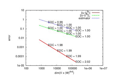
(a) Convergence rates

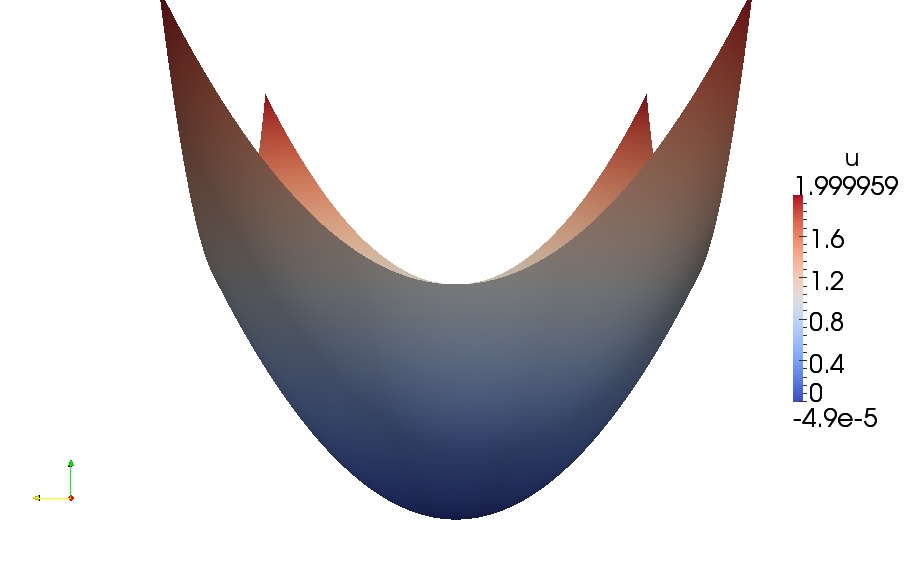
(b) Finite element approximation

Remark 3.1 (on the value of $\tau$).

The optimal values of the timestep parameter or tuning parameter $\tau$ depend upon the regularity of the solution. For example, for a classical solution, one may choose $\tau$ large. In the numerical experiment above we took $\tau=1000$. Since the linearisation is nothing more than seeking the steady state of the evolution equation (9). The convergence (in $n$) is extremely quick taking no more than five iterations.

For the examples below one must be careful choosing $\tau$, we will be looking at viscosity solutions that are not $\operatorname{C}^{2}(\Omega)$, in this case the lack of regularity of the solution will lead to an unstable linearisation for large $\tau$. In each of the cases below $\tau\in[1:10]$ was sufficiently small to achieve convergence of the linearisation in at most twenty iterations.

3.0.2 A known viscosity solution to the homogeneous problem

To test the convergence of the method applied to a singular solution of the homogeneous problem we fix

$$f\equiv 0\text{ and }g=\left|x\right|^{4/3}-\left|y\right|^{4/3},$$ (22)

where $\boldsymbol{x}={\!\left({x,y}\right)}^{{\boldsymbol{\intercal}}}$. A known viscosity solution of this equation is the Aronsson solution [1],

$$u(\boldsymbol{x})=\left|x\right|^{4/3}-\left|y\right|^{4/3}.$$ (23)

The function has singular derivatives about the coordinate axis, in fact $u\in\operatorname{C}^{1,1/3}(\Omega)$. Figure 2 details a numerical experiment on this problem.

In Figure 3 we conduct an adaptive experiment based on the newest vertex bisection method.

Figure 2: We benchmark problem (22), plotting the log of the error together with its estimated order of convergence. We examine both $\operatorname{L}_{2}(\Omega)$ and $\operatorname{H}^{1}(\Omega)$ norms of the error together with the residual estimator given in Theorem 2.7. We choose $\tau=1$ and the linearisation tolerance is coupled to the mesh-size such that the linearisation is run until $\left\|U^{n}-U^{n-1}\right\|\leq 10h^{2}$. The convergence rates are suboptimal due to the singularity, that is, $\left\|u-U^{N}\right\|\approx\operatorname{O}(h^{1.8})$ and $\left|u-U^{N}\right|_{1}\approx\operatorname{O}(h^{0.8})$.

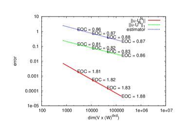
(a) Convergence rates

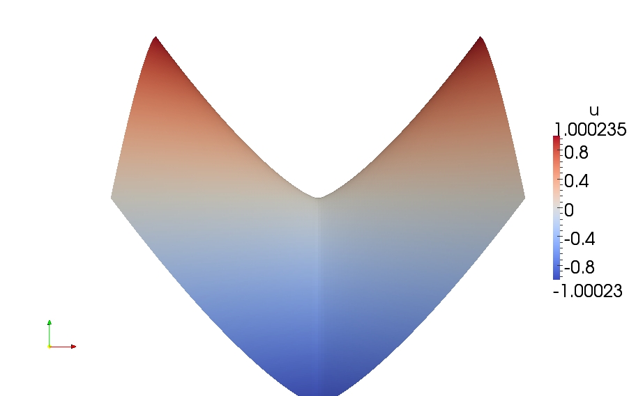
(b) Finite element approximation

Figure 3: This is an adaptive approximation of the viscosity solution $u=\left|x\right|^{4/3}-\left|y\right|^{4/3}$ from (22). The estimator tolerance was set at $0.1$ to coincide with the final estimate from the benchmark solution from Figure 2. The final number of degrees of freedom was $36,325$ compared to the uniform scheme which took $165,125$ degrees of freedom to reach the same tolerance. We chose $\tau=0.1$ as the timestep parameter.

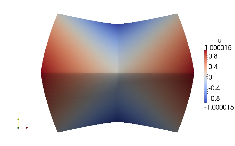
(a) The finite element approximation viewed from the top.

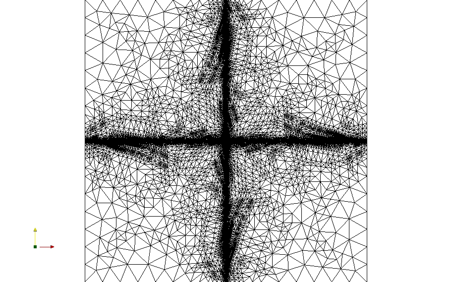
(b) The underlying mesh

References

- [1] G. Aronsson, Construction of singular solutions to the -harmonic equation and its limit equation for , Manuscripta Math. 56:2 (1986), 135–158.
- [2] G. Awanou, Pseudo time continuation and time marching methods for Monge–Ampère type equations, In revision - tech report available on http://www.math.niu.edu/awanou/ (2012).
- [3] E. N. Barron, L. C. Evans, and R. Jensen, The infinity Laplacian, Aronsson’s equation and their generalizations, Trans. Amer. Math. Soc. 360:1 (2008), 77–101.
- [4] L. A. Caffarelli and X. Cabré, Fully nonlinear elliptic equations, American Mathematical Society Colloquium Publications, vol. 43, American Mathematical Society, Providence, RI, 1995.
- [5] M. G. Crandall, L. C. Evans, and R. F. Gariepy, Optimal Lipschitz extensions and the infinity Laplacian, Calc. Var. Partial Differential Equations 13:2 (2001), 123–139.
- [6] M. G. Crandall, H. Ishii, and P.-L. Lions, User’s guide to viscosity solutions of second order partial differential equations, Bull. Amer. Math. Soc. (N.S.) 27:1 (1992), 1–67.
- [7] A. Dedner and T. Pryer, Discontinuous Galerkin methods for nonvariational problems, Submitted - tech report available on ArXiV http://arxiv.org/abs/1304.2265 (2013).
- [8] S. Esedoglu and A. M. Oberman, Fast semi-implicit solvers for the infinity laplace and p-laplace equations, Arxiv (2011).
- [9] L. C. Evans and O. Savin, regularity for infinity harmonic functions in two dimensions, Calc. Var. Partial Differential Equations 32:3 (2008), 325–347.
- [10] X. Feng and M. Neilan, Vanishing moment method and moment solutions for fully nonlinear second order partial differential equations, J. Sci. Comput. 38:1 (2009), 74–98.
- [11] R. Jensen, Uniqueness of Lipschitz extensions: minimizing the sup norm of the gradient, Arch. Rational Mech. Anal. 123:1 (1993), 51–74.
- [12] O. Lakkis and T. Pryer, A finite element method for second order nonvariational elliptic problems, SIAM J. Sci. Comput. 33:2 (2011), 786–801.
- [13] G. Lu and P. Wang, Inhomogeneous infinity Laplace equation, Adv. Math. 217:4 (2008), 1838–1868.
- [14] A. M. Oberman, A convergent difference scheme for the infinity Laplacian: construction of absolutely minimizing Lipschitz extensions, Math. Comp. 74:251 (2005), 1217–1230 (electronic).