Probing nonlinear adiabatic paths with a universal integrator

Abstract

We apply a flexible numerical integrator to the simulation of adiabatic quantum computation with nonlinear paths. We find that a nonlinear path may significantly improve the performance of adiabatic algorithms versus the conventional straight-line interpolations. The employed integrator is suitable for solving the time-dependent Schrödinger equation for any qubit Hamiltonian. Its flexible storage format significantly reduces cost for storage and matrix-vector multiplication in comparison to common sparse matrix schemes.

Simulating quantum systems requires enormous computational resources: Even for a few hundred particles there would be more variables to be stored than atoms exist in the universe Stolze and Suter (2003). To turn this problem into an advantage, quantum computers may be efficiently used for such simulations, since they are quantum systems themselves Feynman (1982). Moreover, quantum algorithms can solve distinct problems like number factoring with exponential speedup compared to classical computers Shor (1997).

In the conventional picture, quantum algorithms are implemented as a sequence of unitary operations Nielsen and Chuang (2000), which implies fast switching of the generating Hamiltonian. In contrast, within the paradigm of adiabatic quantum computation Farhi et al. (2001), the Hamiltonian is modified slowly from a simple initial Hamiltonian with an easy-to-prepare ground state to a final Hamiltonian which encodes in its ground state the solution to some difficult problem. Most importantly, for a large class of problems, implementation of the final Hamiltonian is possible without knowing the solution of the problem explicitly. The adiabatic theorem implies – provided the evolution is slow enough – that the system will end up near the ground state of the final Hamiltonian, such that the solution to the problem can be obtained by measuring the system. The evolution time is related to the spectral properties of the time-dependent Hamiltonian and thus corresponds to the algorithmic complexity of an adiabatic quantum algorithm (AQA). The conventional circuit picture and the adiabatic approach are known to be polynomially equivalent Aharonov et al. (2007); Mizel et al. (2007), but exact results for adiabatic algorithms are scarce Roland and Cerf (2002). It is therefore quite interesting that first numerical simulations of the Schrödinger equation revealed a seemingly polynomial complexity of the adiabatic algorithm for an NP-complete problem Farhi et al. (2001). Since then, it has been a strongly debated question whether this scaling would persist for larger problem sizes Boulatov and Smelyanskiy (2003); Znidaric and Horvat (2006); Ioannou and Mosca (2008); Young et al. (2008); Amin and Choi (2009); Schaller and Schützhold (2010). Recent findings suggest that the scaling complexity of the conventional straight-line adiabatic interpolation is typically exponential Altshuler et al. (2010); Young et al. (2010). It may however be conjectured that with modifications of the adiabatic algorithm, its scaling behavior can be considerably improved Farhi et al. (2008), such that the scaling behavior of adapted algorithms is still an open question.

Unfortunately, this question can currently not be settled from the experimental side: Though enormous progress has been made in the last decade, not more than a few quantum bits (qubits) have been entangled so far Monz et al. (2011), which currently restricts the execution of quantum algorithms to proof-of-principle demonstrations. As experiments are still neither flexible nor scalable enough to investigate new theoretical models, the demand for classical computer simulations of quantum algorithms is growing. Such simulations are computationally expensive and usually must be coded separately for each problem considered. Here, we use an efficient numerical integrator to solve the time-dependent Schrödinger equation for the high-dimensional but sparse Hamiltonians typical for qubit systems. An adopted storage format will reduce the memory required for storing the Hamiltonian in comparison to common sparse matrix schemes while keeping their advantage of fast matrix-vector multiplication. In particular its ability to follow flexible adiabatic paths renders our storage scheme suitable for such simulations.

The paper is structured as follows: In Sec. I, we expose the prerequisites discussing the data storage scheme, adiabatic computation, and the particular NP-complete problem considered. Afterwards, we numerically compare the performance of different adiabatic quantum algorithms (AQAs) for straight-line interpolation in Sec. II. Then, we turn to the investigation of non-linear paths in Sec. III and close with conclusions.

I Theory

I.1 Sparse Quantum Hamiltonian (SQH)

A single-qubit state is a superposition of two fundamental states denoted by $\left|0\right>$ and $\left|1\right>$, which form the computational basis. As a convention, those states are the eigenstates of the Pauli matrix $\sigma^{z}$: $\left|0\right>:=\left(\begin{smallmatrix}1\\ 0\end{smallmatrix}\right),\;\left|1\right>:=\left(\begin{smallmatrix}0\\ 1\end{smallmatrix}\right)$. Similarly, the basis states for an $n$-qubit system can be constructed by the tensor product

$$\left|z\right>=\bigotimes_{i=1}^{n}\left|z_{i}\right>,\;z_{i}\in\{0,1\}.$$ (1)

Here $z$ is the decimal representation $z=\sum_{i=1}^{n}z_{i}\,2^{i-1}$ of the bitstring $z_{n}\,z_{n-1}\ldots z_{2}\,z_{1}$. An arbitrary $n$-qubit state is then given by the superposition

$$\left|\psi\right>=\sum_{z=0}^{2^{n}-1}\alpha_{z}\left|z\right>,\;\alpha_{z}\in\mathds{C}$$ (2)

with normalization condition $\sum_{z}\left|\alpha_{z}\right|^{2}=1$. Obviously, the dimension of the Hilbert space, $N=2^{n}$, is growing exponentially with the number of qubits which makes simulations of quantum systems hard.

A Hamiltonian acting on $n$ qubits can be described by the Pauli matrices $\sigma^{x},\sigma^{y},\sigma^{z}$: Together with the identity $\sigma^{0}:=\mathds{1}$ they span the space of all $2\times 2$-matrices. Using the $n$-fold Kronecker product of those matrices yields $N^{2}=2^{2n}$ generalized Pauli matrices (GPMs) $\mathcal{S}_{i}=\bigotimes_{q=1}^{n}\sigma^{\alpha_{i,q}}$ as a basis for all $N\times N$-matrices. Trace-orthogonality ensures that any Hamiltonian can be decomposed into GPMs,

$$\mathcal{H}=\sum_{i=0}^{N^{2}-1}m_{i}\,\mathcal{S}_{i}\quad\text{with}\quad m_{i}=\frac{1}{N}\mathrm{Tr}\{\mathcal{H}\,\mathcal{S}_{i}\}\in\mathds{R}.$$ (3)

Let $\sigma_{i}^{\alpha}$ be the short notation of the tensor product

$$\underbrace{\mathds{1}\otimes\ldots\otimes\mathds{1}}_{i-1}\otimes\;\sigma^{\alpha}\otimes\underbrace{\mathds{1}\otimes\ldots\otimes\mathds{1}}_{n-i},\qquad\alpha\in\{x,y,z\},$$ (4)

acting only on the $i$-th qubit. A GPM of order $j$ (acting non-trivially on $j$ qubits) is then written as $\sigma_{i_{1}}^{\alpha_{1}}\sigma_{i_{2}}^{\alpha_{2}}\ldots\sigma_{i_{j}}^{\alpha_{j}}$. By counting only non-vanishing terms $m_{i}\neq 0$, Eq. (3) has the more convenient form

$$\mathcal{H}=m^{(0)}\mathds{1}+\sum_{j=1}^{p}\sum_{l=1}^{k_{j}}m_{l}^{(j)}\prod_{q=1}^{j}\sigma_{i_{l,q}^{(j)}}^{\alpha_{l,q}^{(j)}}\,,$$ (5)

where $p$ denotes the order of the Hamiltonian, $k_{j}$ the number of $j$-local terms, $m_{l}^{(j)}$ the corresponding real prefactor, and $m^{(0)}$ the energy shift.

We now introduce a Sparse Quantum Hamiltonian (SQH) format: For a complete description of the Hamiltonian’s structure, we do not need to store the full GPMs but only the parameters used in Eq. (5), including the positions $i$ and types $\alpha$ of the (single) Pauli matrices. Consequently, storage of a Hamiltonian is efficient if its order is independent of the number of qubits, $p\ll n$, and becomes even more favorable when the number of terms for every order $j$ is small, e.g., $k_{j}\sim{\cal O}(n)$. An example of such a system is the quantum Ising model in a transverse field,

$$\mathcal{H}=-\Omega(1-s)\sum_{i}^{n}\sigma_{i}^{x}-\Omega s\sum_{i}^{n}\sigma_{i}^{z}\sigma_{i+1}^{z}\,,$$ (6)

where $\Omega$ represents an energy scale and $s$ a control parameter and where periodic boundary conditions are assumed $\sigma^{z}_{n+1}=\sigma^{z}_{1}$. This Hamiltonian would only require ${\cal O}(n)$ elements to store in SQH format.

A matrix-vector product $\mathcal{H}\left|\psi\right>$ is according to Eq. (5) reduced to a sum of GPMs acting on a basis state, $\sigma_{i_{1}}^{\alpha_{1}}\ldots\sigma_{i_{j}}^{\alpha_{j}}\left|z\right>$. Due to the tensor structure of $z$ (c.f. Eq. (1)), such a multi-qubit operation is broken down to a multiplication of successive single-qubit operations $\sigma_{i}^{\alpha}\left|z_{i}\right>$. Assuming the number of terms in $\mathcal{H}$ is ${\cal O}(n)$, the effort for computing $\mathcal{H}\left|\psi\right>$ scales as $N\times{\cal O}(n)$ instead of $N^{2}$ when the Hamiltonian was stored conventionally.

The universal applicability of the SQH representation allows to write program code (e.g., an integrator) independent of the used Hamiltonian as long as it has the SQH structure given in Eq. (5). Also time-dependent Hamiltonians can be implemented by time-dependent coefficients $m_{l}^{(j)}(t)$.

I.2 Adiabatic Quantum Computation

Quantum computation by adiabatic evolution has been suggested as a promising approach for solving NP-complete problems Farhi et al. (2001). The idea is simple: A final Hamiltonian ${\mathcal{H}}_{f}$ is constructed which encodes the solution for a computational problem in its ground state, e.g., as an energy penalty function. We stress here that for a number of hard problems this can be done without knowing the solution. Starting from an easy to construct ground state of an initial Hamiltonian ${\mathcal{H}}_{i}$, the system is transformed to ${\mathcal{H}}_{f}$ after the runtime $T$. A common approach is to use a linear interpolation:

$$\mathcal{H}(s)=(1-s){\mathcal{H}}_{i}+s{\mathcal{H}}_{f}$$ (7)

with constant velocity $s(t)=\frac{t}{T}$ and $0\leq t\leq T$. If this transformation is slow enough, the adiabatic theorem guarantees that the system remains always near the instantaneous ground state Sarandy et al. (2004) such that a measurement after time $T$ yields the solution. This works in principle with every energy eigenstate of the system, but by using the ground state one hopes that the evolution is dissipation-free (which becomes relevant when the system is coupled to a low-temperature reservoir Childs et al. (2001)). The runtime $T$ thus is a measure for the algorithmic complexity. It can be optimized by adapting the speed of the interpolation $\dot{s}(t)$ to the energy gap above the ground state Roland and Cerf (2002); Jansen et al. (2007); Schaller et al. (2006). In this case however, the time-dependent Hamiltonian is still a convex combination of initial and final Hamiltonian (hence the terminology straight-line interpolations), and we will not consider such extensions here.

To study the efficiency of such an algorithm, i.e., the runtime scaling with increasing system size $n$, we need to determine an adiabatic runtime $T_{s}(n)$ by simulating the evolution of a system prepared in the initial ground state. It is governed by the Schrödinger equation

$$i\hbar\frac{\mathrm{d}}{\mathrm{d}t}\left|\psi(t)\right>=\mathcal{H}{(t)}\left|\psi(t)\right>,$$ (8)

which for the expansion in Eq. (2) becomes a whole set of $N$ coupled ordinary differential equations with initial condition $\left|\psi(0)\right>=\left|\psi_{0}\right>$. A fast numerical integration is achieved by using the SQH format for $\mathcal{H}(t)$ and a fourth-order predictor-corrector scheme Gershenfeld (2000), which requires only a single evaluation of $\mathcal{H}\left|\psi\right>$ per integration step.

I.3 3-Bit Exact Cover

A common problem for probing adiabatic quantum algorithms (AQAs) is 3-bit exact cover (EC3), which is NP-complete. In a nutshell, solutions to problems in the class NP can be verified (with a classical computer) in a time that is polynomial in the length of their input. The completeness property in addition implies that every other problem in NP can be mapped to EC3 with polynomial overhead only.

On an $n$-bitstring $z_{n}\,z_{n-1}\ldots z_{2}\,z_{1}$ we define an instance of EC3 as a set of $m$ different clauses $c_{i}$ each involving three different bits

$$c_{i}=(c_{i}^{(1)},c_{i}^{(2)},c_{i}^{(3)}),\qquad c_{i}^{(k)}\in\{1\ldots n\}$$ (9)

with $1\leq i\leq m$. A clause is satisfied, if and only if one of the involved bits $z_{i}$ equals 1, i.e., when

$$z_{c_{i}^{(1)}}+z_{c_{i}^{(2)}}+z_{c_{i}^{(3)}}=1\,,$$ (10)

where ’$+$’ denotes the ordinary integer sum. A solution to an instance is a bitstring satisfying all clauses in the set, which is easy to check. In contrast, finding such a bitstring is a combinatorial search problem for which no efficient classical algorithm is known. Figure 1 visualizes an EC3 instance for 13 bits with a unique solution.

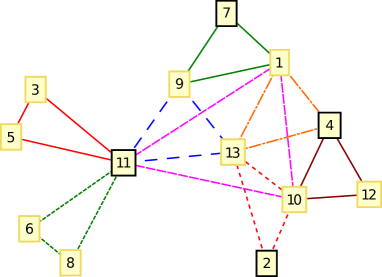
Figure 1: (Color Online) Instance of EC3, where the labeled vertices represent the 13 bits $z_{i}$, edges of same color and line style represent a clause $c_{i}$. Bold-bordered vertices indicate the upbits in the solution $z=1098=(0010001001010)$.

For an AQA the problem is encoded as a cost function, where each unsatisfied clause adds an energy penalty to the Hamiltonian Banuls et al. (2006),

$$h_{i}=\left[\mathds{1}-\frac{1}{2}\sum_{k}^{3}\left(\mathds{1}-\sigma^{z}_{c_{i}^{(k)}}\right)\right]^{2}.$$ (11)

The final Hamiltonian ${\mathcal{H}}_{f}$ is simply constructed as a sum over all clauses and can be simplified to Schützhold and Schaller (2006)

$${\mathcal{H}}_{f}=\sum_{i=1}^{m}\Omega h_{i}=\Omega m\mathds{1}-\Omega\sum_{i}^{n}\frac{n_{i}}{2}\sigma_{i}^{z}+\Omega\sum_{i<j}^{n}\frac{n_{i,j}}{2}\sigma_{i}^{z}\sigma_{j}^{z}.$$ (12)

Here, $\Omega>0$ just denotes an energy scale, the coefficient $n_{i}$ denotes the number of clauses involving the i-th qubit, and $n_{i,j}$ is the number of clauses, which contain the $i$-th and $j$-th qubit. For example, in Fig. 1 we have $n_{11}=4$ and $n_{11,13}=1$. The Hamiltonian ${\mathcal{H}}_{f}$ corresponds to a frustrated antiferromagnet in a non-uniform magnetic field (with an energy shift $m$) Schützhold and Schaller (2006). The coupling strength between the spins, however, is not defined by the experimental geometry (e.g., only between nearest neighbors) but by the edges of the clauses $n_{i,j}$, which may define a highly disordered network.

I.4 Hard Instances

To provide statistical evidence for our simulations, we generate for each system size 100 hard instances. These were characterized by a unique solution, a number of clauses close to the classical EC3 phase transition $m\approx\frac{2}{3}n$ from satisfiable to unsatisfiable problems Kalapala and Moore (2005), and the constraint that $n_{ij}\in\{0,1\}$. The last constraint implies that clauses should only share vertices and not edges. It is motivated by the fact that in case an edge is shared by two clauses, one may easily conclude that in the solution, the opposite vertices must have the same value. Effectively, clauses that share edges would thus reduce the size of the problem. Altogether, these constraints lead to ${\cal O}(n)$ terms in Eq. (12), and ${\mathcal{H}}_{f}$ is efficiently stored in SQH format.

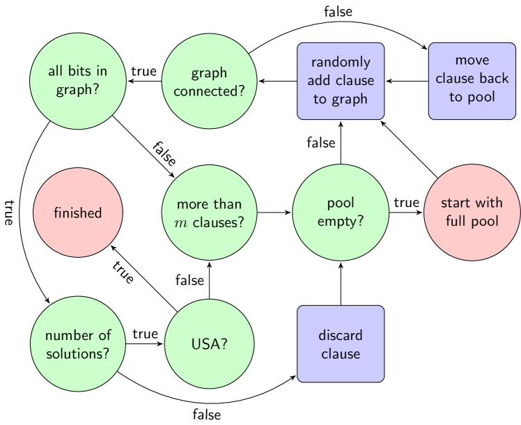
Figure 2: (Color Online) Scheme of the used algorithm for randomly generating hard instances of EC3. Rectangles and circles indicate instructions and if-clauses, respectively. The algorithm starts and stops at diamonds.

The recipe for generating a random (hard) instance is shown in figure 2. We start with a full pool of all possible clauses. Randomly choosing one of the clauses defines an initial graph – a triangle. This graph is now iteratively increased by randomly choosing among the remaining clauses whilst obeying simple rules: First, only clauses which intersect with the existing graph are added to ensure connectivity. When all bits are connected to the graph, the number of solutions is checked each time after a clause is drawn. A clause is discarded, if it reduces the number of solutions to zero. The algorithm finishes if only one solution is left. If no such unique satisfying assignment (USA) has been found but all clauses are dropped from the pool or the number of allowed clauses $m$ is reached, the algorithm restarts itself.

II Straight Line Interpolation

In this section, we simulate and compare the results of three AQAs defined by different initial Hamiltonians ${\mathcal{H}}_{i}$. The interpolation path between initial and final Hamiltonian is a straight line given by Eq. (7), traversed at constant speed $s(t)=t/T$. As a benchmark, we compare with the analytically solvable Ising model in Eq. (6), which exhibits an inverse $1/n$-scaling of the minimum energy gap between ground and first coupled excited state, leading to a quadratic scaling of the adiabatic runtime Dziarmaga (2005). We begin by summarizing the explored algorithms.

II.1 Algorithms

II.1.1 X-Algorithm

The original approach Farhi et al. (2001) used a single-qubit structure

$${\mathcal{H}}_{i}=\mathcal{H}^{x}=\Omega\sum_{i}^{n}\frac{n_{i}}{2}(\mathds{1}-\sigma_{i}^{x})$$ (13)

with the ground state

$$\left|S\right>=\frac{1}{\sqrt{2^{n}}}\sum_{z=0}^{N-1}\left|z\right>.$$ (14)

However, this does not reflect the interaction topology of the final Hamiltonian (12), i.e., the coefficient $n_{i}$ does not carry the full information about the clauses $c_{i}$.

II.1.2 XYZ-Algorithm

A choice with two-qubit interactions is the Heisenberg ferromagnet Schützhold and Schaller (2006); Schaller and Schützhold (2010)

$${\mathcal{H}}_{i}=\mathcal{H}^{xyz}=\Omega\sum_{i<j}^{n}\frac{n_{i,j}}{2}(\mathds{1}-\boldsymbol{\sigma}_{i}\cdot\boldsymbol{\sigma}_{j}).$$ (15)

Both $\mathcal{H}^{xyz}$ and ${\mathcal{H}}_{f}$ are invariant under rotations around the $\Sigma^{z}$-axis,

$$\Sigma^{z}=\sum_{i}^{n}\frac{1}{2}(\mathds{1}-\sigma_{i}^{z}).$$ (16)

The eigenvalue $\Delta$ of $\Sigma^{z}$ is directly related to the number of $1$-bits in the solution (also denoted as Hamming weight $\Delta$). It is therefore a constant of motion and conserved during dynamics. Only the subspace $\left|\psi\right>:\Sigma^{z}\left|\psi\right>=\Delta_{w}\left|\psi\right>$ with the fixed Hamming weight $\Delta_{w}$ of the solution has to be considered here, as all subspaces with different Hamming weights evolve independently. The ground state of $\mathcal{H}^{xyz}$ in the appropriate subspace is given by a balanced superposition over all basis states $\left|u\right>$ with $\Sigma^{z}\left|u\right>=\Delta_{w}\left|u\right>$,

$$\left|\psi_{0}\right>^{xyz}=\begin{pmatrix}n\\ \Delta_{w}\end{pmatrix}^{-\frac{1}{2}}\sum_{u}\left|u\right>.$$ (17)

which can be prepared efficiently Childs et al. (2002) by adiabatic evolution $\mathcal{H}^{x}\overset{T}{\rightarrow}\mathcal{H}^{P}$. In that reference, the final Hamiltonian $\mathcal{H}^{P}$ used an energy penalty to separate the subspaces: It was given by $\mathcal{H}^{P}=\left(\Sigma^{z}-\Delta_{w}\right)^{2}$, which has highly degenerate energy levels, but due to symmetry arguments the correct angular momentum eigenstates were selected. In our numerical considerations we circumvent this preparation step and directly prepare the initial state (17), such that the adiabatic algorithm only consists in a deformation of $\mathcal{H}^{xyz}$ to the final problem Hamiltonian (12).

Realistically, the solution $\left|w\right>$ and thus the Hamming weight $\Delta_{w}$ would not be known in advance, which would make repeated runs of the AQA in different subspaces necessary. But even in the worst case, when every possible value of $\Delta\in\{0\ldots n\}$ has to be tried, the computational overhead scales only linearly in $n$.

II.1.3 XY-Algorithm

Similar to the previous example is the x,y-ferromagnet

$${\mathcal{H}}_{i}=\mathcal{H}^{xy}=3m\Omega\mathds{1}-\Omega\sum_{i<j}^{n}\frac{n_{i,j}}{2}(\sigma_{i}^{x}\sigma_{j}^{x}+\sigma_{i}^{y}\sigma_{j}^{y}).$$ (18)

It has already been shown numerically that it yields on average a better performance than $\mathcal{H}^{xyz}$ on a common instance of EC3 with a unique solution Schützhold and Schaller (2006). Again, the Hamming weight is a constant of motion and we only consider the corresponding subspace. The ground state of (18) is analytically unknown but can be initialized by adiabatic evolution $\mathcal{H}^{x}\overset{T}{\rightarrow}\mathcal{H}^{xy}$. Using an ARPACK eigensolver Lehoucq et al. (1998); Kandler and Schröder (2013) accepting SQH as input variable, we found numerically for the examples considered that the minimum gap during the initial preparation is roughly independent of the system size. We expect therefore only a mild algorithmic scaling of this preparation step with the system size $n$, which would enable an efficient adiabatic preparation of the ground state of Eq. (18).

II.2 Results

The probability to find the system in the solution state $\left|w\right>$ after the runtime $T$ is $P_{1}(T)={\left|\left<\psi(T)|w\right>\right|}^{2}$ and would ideally approach one. However, to avoid too long computation times but simultaneously ensure a high fidelity, we define a successful runtime $T_{s}$ by measuring the system’s energy $E(T_{s})/\Omega=\frac{1}{2}$. Here, we exploit the fact, that any excited state raises the energy by an amount greater or equal $\Omega$, cf. Eq. (12). The first excited state of ${\mathcal{H}}_{f}$ therefore has an energy $E_{2}\geq\Omega$. The energy is thus lower bounded by (using $E_{1}(T)=0$)

$$E(T) = \sum_{n=1}^{N}E_{n}(T)P_{n}(T)\geq E_{2}(P_{2}+\ldots+P_{N})$$ (19)

$$\geq \Omega(1-P_{1})\,,$$

and defining this criterion as a measure for a successful runtime means that the ground state occupation is at least one-half.

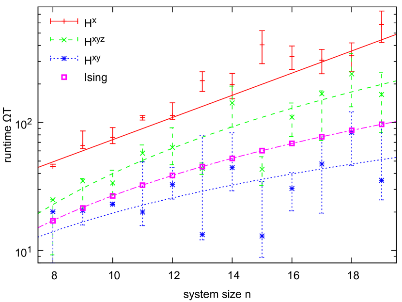
Figure 3: (Color Online) Scaling of the dimensionless runtime $\Omega T_{s}(n)$ (symbols, fit lines only serve to guide the eye) for algorithms X (solid), XYZ (long-dashed), XY (dotted) compared with the quadratically scaling Ising model (dash-dotted). Symbols represent the median and error bars the first and third quartile out of 100 randomly chosen hard instances. Although the scaling behavior is inconclusive, it is evident that different initial states may drastically improve the performance of the AQA.

Figure 3 shows computed median runtimes $T_{s}(n)$ for the three different algorithms compared with an adiabatic version of the Ising model, Eq. (6), traversed at constant interpolation speed $s(t)=t/T$. The latter serves as a benchmark with a runtime scaling known to be quadratically Dziarmaga (2005). Our results show, that the XY-algorithm is the fastest followed by the XYZ-algorithm. Both stay close to the Ising curve which would indicate a polynomial scaling in the observed region. A clear statement however is hampered by the large deviations and fitting remains ambiguous. In contrast to previous studies Farhi et al. (2001), where the runtime of the X-algorithm appeared polynomial on small system sizes, our results on harder instances suggest an exponential scaling of the original algorithm already for these moderate sizes $n$.

III Alternative Paths

A straight line interpolation between initial Hamiltonian ${\mathcal{H}}_{i}$ and final Hamiltonian ${\mathcal{H}}_{f}$ is a convex combination of only of two Hamiltonians. However, there are plenty of other paths connecting these two but involving a third or even more intermediate Hamiltonians. Our hope is, that some of such alternative paths may increase the energy gap above the ground state leading to a speedup of the AQA. For example, in the simple Ising model (6) it is known that even for constant-speed interpolations $s(t)=t/T$, the runtime can be improved from quadratic scaling (straight line) to linear scaling (nonlinear path) Schaller (2008). Since the XY-algorithm showed the best median performance in the previous section, we set the initial Hamiltonian to $\mathcal{H}^{xy}$ and probe two alternative algorithms based on paths shown in Fig. 4.

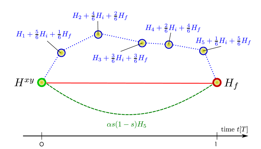
Figure 4: (Color Online) Sketch of alternative paths for adiabatic algorithms all starting from $\mathcal{H}^{xy}$. As an example, the number of clauses is set to $m=6$. The red, solid line is the straight line algorithm. The green, dashed curve denotes a path with an additional, nonlinear term $s(1-s)H_{5}$, which is defined in the text. A clause-by-clause algorithm is shown by the blue, dotted lines.

III.1 Algorithms

III.1.1 Nonlinear Smooth Interpolation

We add a third term to the straight line interpolating Hamiltonian $\mathcal{H}(s)$ in Eq. (7), which is quadratic in $s$:

$$\mathcal{H}(s)=(1-s)\mathcal{H}^{xy}+s{\mathcal{H}}_{f}+\alpha s(1-s)\mathcal{H}_{m-1},$$ (20)

where $\mathcal{H}_{m-1}=\Omega\sum_{i=1}^{m-1}h_{i}$ is the final Hamiltonian reduced by one (arbitrarily chosen) clause and $\alpha$ is a coupling strength. To motivate this path, we note that for large $n$, the related reduced EC3 problem may be expected to have many solutions, since there exists a phase transition from satisfiable to unsatisfiable EC3 problems at a clause-to-size ratio $m/n\approx 0.62$ Kalapala and Moore (2005). Thus, reducing the number of clauses moves the problem into the satisfiable phase. Intuitively, we expect that the additional term in Eq. (20), which becomes dominant during the evolution, will already at this state suppress states which are not a solution to $\mathcal{H}_{m-1}$ (and therefore neither of $\mathcal{H}_{m}$). Thereby, the search space to find the solution of ${\mathcal{H}}_{f}$ is reduced, and the algorithm could be expected to be faster compared to conventional straight line interpolation.

It should be noted, that for $m$ clauses there are $m$ different Hamiltonians $\mathcal{H}_{m-1}$. The best reduction of the search space is then obtained for reduced Hamiltonians $\mathcal{H}_{m-1}$ with the smallest number of solutions. However, this number will in realistic experiments not be known. In our numerical simulations, we have decided to remove only clauses when the connectivity of the graph is not destroyed. In the example of Fig. 1, allowed clauses to be removed are $(1,4,13),(1,10,11)$ and $(9,11,13)$.

III.1.2 Nonlinear Clause-By-Clause Interpolation

We try again to reduce to search space by applying an additional term to the straight line interpolation. In contrast to the previous case however, the reduction is conducted not in a single step but by switching on the clauses one after another. This can be written formally as

$$\mathcal{H}(s) =(1-s)\mathcal{H}^{xy}+s{\mathcal{H}}_{f}+\mathcal{H}_{d}(s),$$ (21)

$$\mathcal{H}_{d}(s) =\sum_{k=1}^{m}\begin{aligned} &\big{[}(1-s_{k})\mathcal{H}_{k-1}+s_{k}\mathcal{H}_{k}\big{]}\\[2.84526pt] &\times\Theta(s_{k})\Theta(1-s_{k}),\end{aligned}$$ (22)

$$\text{where}\qquad s_{k} =ms-k+1.$$ (23)

The primary interpolation $s:0\rightarrow 1$ of Eq. (21) is thus split into $m$ steps, which consist of secondary interpolations $s_{k}:0\rightarrow 1$ from $\mathcal{H}_{k-1}$ to $\mathcal{H}_{k}$ in Eq. (22). Here, $\mathcal{H}_{k}$ consists of $k$ clauses from ${\mathcal{H}}_{f}$. Note that this is equivalent to adding a single clause with each step denoted by $\mathcal{H}_{k}-\mathcal{H}_{k-1}$. As the initial and final Hamiltonians, $\mathcal{H}(0)=\mathcal{H}^{xy}$ and $\mathcal{H}(1)={\mathcal{H}}_{f}$ should not be changed by $\mathcal{H}_{d}$, we define $H_{0}=\mathcal{H}_{m}=0\cdot\mathds{1}$. The order, in which clauses are added, is ambiguous, which results in $m!$ possible paths. In our numerical simulations, the path was defined by the order in which the clauses were stored.

III.2 Results

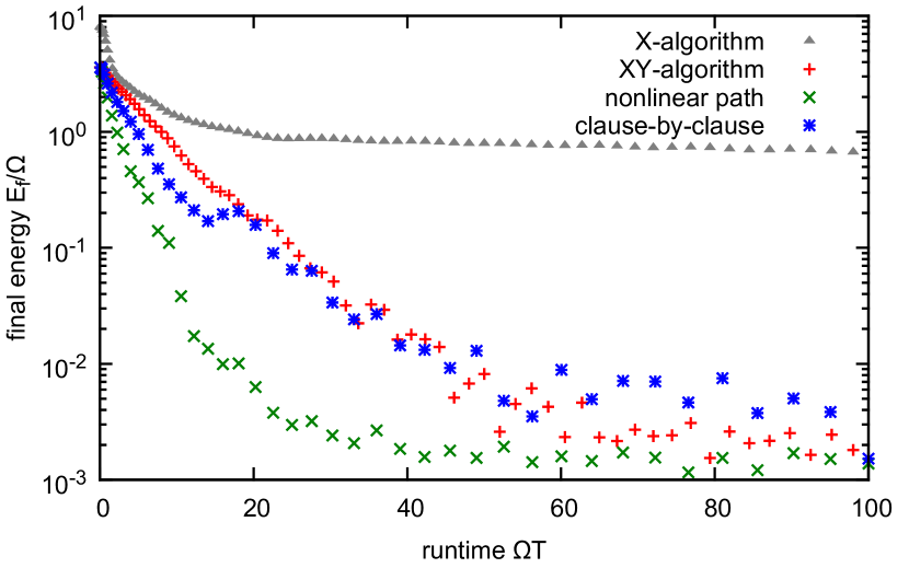
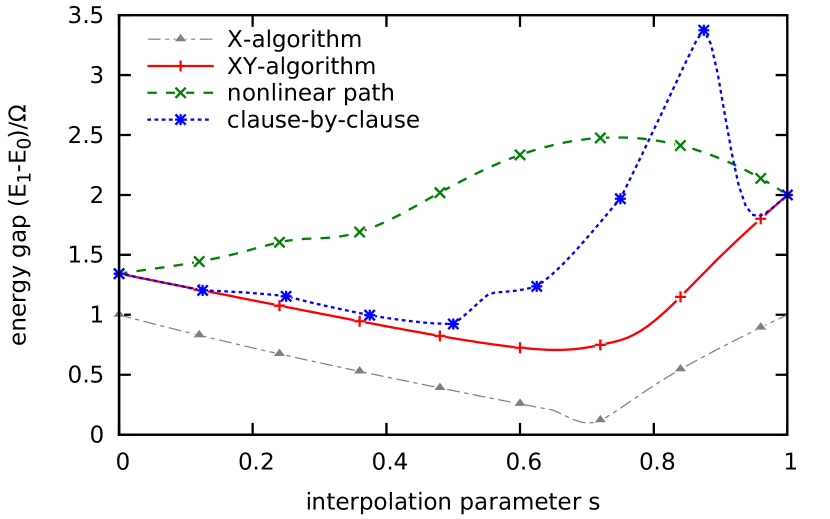
Figure 5: (Color Online) Top: Final energies versus dimensionless runtimes for different paths between $\mathcal{H}^{xy}$ and ${\mathcal{H}}_{f}$ for a 13 qubit example. Symbol shapes and colors correspond to the paths in Fig. 4. The X-algorithm is also shown as an example of a slow adiabatic behavior. For the nonlinear path, the coupling is chosen as $\alpha=8$. Bottom: Energy gap between ground and first excited state of $\mathcal{H}(s)$ for the same algorithms. The symbols for the curves correspond to those in the upper panel. For the clause-by-clause algorithm, the symbols indicate the start and end of the secondary interpolations in (22). Comparing both panels, a correspondance between a large minimal gap and a fast decrease in the final energy is clearly seen.

The qubit system is prepared in the ground state of $\mathcal{H}^{xy}$, which can be done efficiently as stated in section II. We then compare for the presented algorithms the final energy $E_{f}$ of the system after a runtime $T$. For an adiabatic runtime, the energy should be close to 0. Additionally, we numerically Lehoucq et al. (1998) compute the lower part of the spectrum and deduce the energy gap above the ground state for each AQA. Figure 5 exemplarily shows our results for an instance with 13 qubits. First, in the upper panel, it is visible that for short runtimes, the conventional algorithm rapidly decreases its final energy, but it becomes increasingly hard to further reduce the energy below the critical threshold one. Both the clause-by-clause algorithm and the XY-algorithm decrease the final energy significantly faster, but the nonlinear path shows an even better performance (we attribute the final plateaus to imperfect numerical preparation of the initial ground state).

The lower panel in Fig. 5 shows the gap between the two lowest eigenvalues of $\mathcal{H}(s)$ dependent of the interpolation parameter $s:0\rightarrow 1$. For the clause-by-clause algorithm, the points indicate the particular steps where another clause is added. Again, the nonlinear paths shows the best result as its minimum gap is largest. Comparing both panels, it can be clearly seen, that a larger minimum gap leads to a faster decrease in the final energy. Remarkably, the minimum gap for the nonlinear algorithm is located at $s=0$, i.e., it coincides with the gap of $\mathcal{H}^{xy}$.

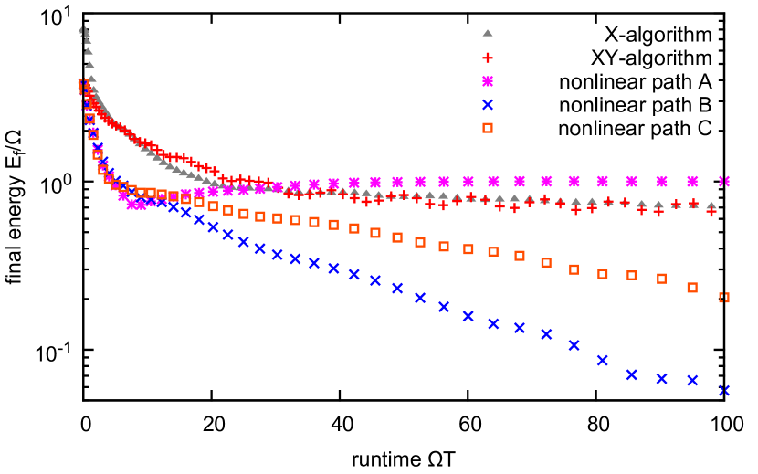
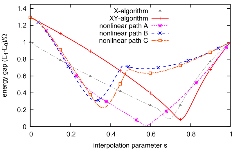
Figure 6: (Color Online) A very hard instance. Top: Final energy of the nonlinear path for different choices of $H_{m-1}$ with coupling $\alpha=8$ compared to the X- and XY-algorithm. Clauses removed from ${\mathcal{H}}_{f}$ for the nonlinear term are $A=(1,10,11),B=(1,4,13)$ and $C=(9,11,13)$. Symbol shapes and colors correspond to the clauses in Fig. 1. Whereas the short-time performance was much better for all nonlinear paths, it turned out that these differ strongly for large evolution times $T$, and choice $A$ performs worse than the straight line interpolations. Bottom: Energy gap for the same algorithms. Again, the value of the minimum gap clearly corresponds to the large-time performance in the above panel. It depends on the choice of $H_{m-1}$ whether this gap is increased or decreased compared to straight line algorithms.

Although a broad statistics would exceed the scope of this paper, we observed a similar behavior for many instances and different system sizes. However, there are very hard instances, where an arbitrarily chosen nonlinear algorithm failed. The graph depicted in Fig. 1 is such an example, which is as hard to solve for the XY-algorithm as it is for the X-algorithm. In this case, our chosen smooth nonlinear path performed for a large coupling constant $\alpha$ even worse.

The choice of the nonlinear term $H_{m-1}$ in (20) turns out to be crucial as shown in Fig. 6. In the upper panel, both straight line algorithms do not reduce the energy significantly below 1. Also shown are the possible three nonlinear paths. Surprisingly, the energy of path A is almost constant 1 for long runtimes. At least two out of three nonlinear paths show a faster decrease in energy than the XY-algorithm, with path B having the best performance. This can be confirmed by examining the energy gap in the lower panel of Fig. 6. The minimum gap of the straight line algorithms is almost identical, whereas the minimum gap of path A is 20 times smaller. Path B has the largest minimum gap as expected.

IV Conclusion

The employed universal integrator proved a flexible tool in simulating non-standard adiabatic quantum algorithms. The introduced SQH format offers an efficient storage scheme and a fast matrix-vector multiplication. Moreover, as the integrator is independent of the Hamiltonian’s structure, it gives the flexibility to simulate hundreds of EC3 instances without changing the source code. Adapting the integrator to alternative interpolating paths could be done very easily.

Our simulations agree with previous results pointing to an exponential scaling of the X-algorithm Znidaric (2005) on hard instances. The performance of the XYZ- and the XY-algorithm is much better, indicating an Ising-like polynomial scaling for the samples and sizes considered. However, we note that variations are large, and the worst-case complexity does not even expose any scaling behavior. Even if this was not the case, finite-size simulations must remain inconclusive by construction. For the alternative paths, we did not study the runtime scaling versus the problem size. Instead, we considered the adiabatic behavior for exemplary instances, where a faster decrease in the final energy corresponds to a larger minimum gap. Here, the nonlinear path outperforms the linear algorithms even for very hard instances. However, in general one will not know in advance, which of the possible choices for the nonlinear path is the best.

For further studies, an analysis of its scaling behavior is of interest. This requires extensive simulations for statistics, which will be a subject of future research.

Our results are of course limited to the specific examples considered, but may give rise to the hope that nonlinear paths may be an interesting road to explore in the field of adiabatic computation.

V Acknowledgments

The authors have profited from discussions with C. Schröder, U. Kandler, R. Okuyama, T. Brandes, V. Mehrmann, R. Schützhold, and F. Renzoni. Financial support by the DFG (BRA-1528/7-1, SCHA 1646/2-1) is also gratefully acknowledged.

References

- Stolze and Suter (2003) J. Stolze and D. Suter, Quantum Computing: A Short Course from Theory to Experiment (Wiley-VCH, 2003).
- Feynman (1982) R. P. Feynman, International Journal for Theoretical Physics 21, 467 (1982).
- Shor (1997) P. W. Shor, SIAM Journal on Computing 26, 1484 (1997).
- Nielsen and Chuang (2000) M. A. Nielsen and I. L. Chuang, Quantum Computation and Quantum Information (Cambridge University Press, Cambridge, 2000).
- Farhi et al. (2001) E. Farhi, J. Goldstone, S. Gutmann, J. Lapan, A. Lundgren, and D. Preda, Science 292, 472 (2001).
- Aharonov et al. (2007) D. Aharonov, W. van Dam, J. Kempe, Z. Landau, S. Lloyd, and O. Regev, SIAM J. Comput. 37, 166 (2007).
- Mizel et al. (2007) A. Mizel, D. A. Lidar, and M. Mitchell, Phys. Rev. Le 99, 070502 (2007).
- Roland and Cerf (2002) J. Roland and N. J. Cerf, Physical Review A 65, 042308 (2002).
- Boulatov and Smelyanskiy (2003) A. Boulatov and V. N. Smelyanskiy, Physical Review A 68, 062321 (2003).
- Znidaric and Horvat (2006) M. Znidaric and M. Horvat, Physical Review A 73, 022329 (2006).
- Ioannou and Mosca (2008) L. M. Ioannou and M. Mosca, International Journal of Quantum Information 6, 419 (2008).
- Young et al. (2008) A. P. Young, S. Knysh, and V. N. Smelyanskiy, Physical Review Letters 101, 170503 (2008).
- Amin and Choi (2009) M. H. S. Amin and V. Choi, Physical Review A 80, 062326 (2009).
- Schaller and Schützhold (2010) G. Schaller and R. Schützhold, Quantum Information and Computation 10, 0109 (2010).
- Altshuler et al. (2010) B. Altshuler, H. Krovi, and J. Roland, PNAS 107, 12446 (2010).
- Young et al. (2010) A. P. Young, S. Knysh, and V. N. Smelyanskiy, Physical Review Letters 104, 020502 (2010).
- Farhi et al. (2008) E. Farhi, J. Goldstone, S. Gutmann, and D. Nagaj, International Journal of Quantum Information 6, 503 (2008).
- Monz et al. (2011) T. Monz, P. Schindler, J. T. Barreiro, M. Chwalla, D. Nigg, W. A. Coish, M. Harlander, W. Hänsel, M. Hennrich, and R. Blatt, Phys. Rev. Lett. 106, 130506 (2011).
- Sarandy et al. (2004) M. S. Sarandy, L.-A. Wu, and D. A. Lidar, Quantum Information Processing 3, 331 (2004).
- Childs et al. (2001) A. M. Childs, E. Farhi, and J. Preskill, Physical Review A 65, 012322 (2001).
- Jansen et al. (2007) S. Jansen, M. B. Ruskai, and R. Seiler, Journal of Mathematical Physics 48, 102111 (2007).
- Schaller et al. (2006) G. Schaller, S. Mostame, and R. Schützhold, Physical Review A 73, 062307 (2006).
- Gershenfeld (2000) N. Gershenfeld, The Nature of Mathematical Modeling (Cambridge University Press, Cambridge, 2000).
- Banuls et al. (2006) M. C. Banuls, R. Orus, J. I. Latorre, A. Perez, and P. Ruiz-Femenia, Physical Review A 73, 022344 (2006).
- Schützhold and Schaller (2006) R. Schützhold and G. Schaller, Physical Review A 74, 060304(R) (2006).
- Kalapala and Moore (2005) V. Kalapala and C. Moore, arXiv: cs.CC, 0508037 (2005).
- Dziarmaga (2005) J. Dziarmaga, Physical Review Letters 95, 245701 (2005).
- Childs et al. (2002) A. M. Childs, E. Farhi, J. Goldstone, and S. Gutmann, Quantum Information and Computation 2, 181 (2002).
- Lehoucq et al. (1998) R. B. Lehoucq, D. C. Sorensen, and C. Yang, ARPACK Users’ Guide: Solution of Large-Scale Eigenvalue Problems with Implicitly Restarted Arnoldi Methods (SIAM, 1998) http://www.caam.rice.edu/software/ARPACK.
- Kandler and Schröder (2013) U. Kandler and C. Schröder, Preprint series of the Institute of Mathematics, TU Berlin , 10 (2013).
- Schaller (2008) G. Schaller, Physical Review A 78, 032328 (2008).
- Znidaric (2005) M. Znidaric, Physical Review A 71, 062305 (2005).