Two-dimensional quasi-ideal Fermi gas with Rashba spin-orbit coupling

Abstract

We investigate the zero-temperature properties of a quasi-ideal Fermi gas with Rashba spin-orbit coupling. We find that the spin-orbit term strongly affects the speeds of zero sound and first sound in the Fermi gas, due to the presence of a third-order quantum phase transition. In addition, including a 2D harmonic confinement we show that also the shape of the density profile of the cloud crucially depends on the strength of the Rashba coupling.

Artificial spin-orbit coupling has been recently implemented in bosonic so-bose ; so-bose2 and fermionic so-fermi1 ; so-fermi2 atomic gases, by means of counterpropagating laser beams which couple two internal hyperfine states of the atom by a stimulated two-photon Raman transition. These experimental achievements have triggered several theoretical investigations in understanding the spin-orbit effects with Rashba rashba and Dresselhaus dress terms in Bose-Einstein condensates stringa1 ; stringa2 ; burrello ; so-solitons ; so-bright1 ; so-bright2 ; so-bright3 ; so-vortices ; so-dipolar and also in the BCS-BEC crossover of superfluid fermions shenoy ; shenoy2 ; gong ; hu ; yu ; iskin ; yi ; dms ; iskin2 ; zhou ; jiang ; sa ; chen ; zhou2 ; yangwan ; iskin3 ; sa2 ; he ; liu ; ne1 ; ne2 .

In this Brief Report we focus on the effects of the Rashba spin-orbit coupling in a normal two-spin-component (i.e. two atomic species) Fermi gas and, for the sake of simplicity and clarity, we consider a two-dimensional (2D) quasi-ideal atomic gas, for which the inter-particle interaction can be neglected in the equation of state. Under the conditions of reduced dimensionality and suppressed inter-particle interaction (see also sala-fermi-reduce ), we analyze theoretically statical and dynamical properties of the system. In particular, after deriving the single-particle density of states of our 2D Fermi gas, we determine the zero-temperature equation of state, namely the chemical potential as a function of the total density and of the Rashba strength. From the equation of state we calculate the speed of sound both in the collisionless regime (zero sound) and collisional regime (first sound). Then we switch on a trapping harmonic potential in the 2D Fermi gas showing how the density profile of the fermionic cloud depends on the Rashba coupling.

The two-spin-component single-particle quantum Hamiltonian ${\hat{h}}_{sp}$ of a confined two-component 3D Fermi gas of identical atoms with mass $m$ and Rashba spin-orbit coupling reads

$${\hat{h}}_{sp}=\left({{\hat{p}}^{2}\over 2m}+U({\bf r})\right)\,\sigma_{0}+v_{R}\ \left(\sigma_{x}{\hat{p}}_{y}-\sigma_{y}{\hat{p}}_{x}\right)\;,$$ (1)

where $U({\bf r})$ is the trapping potential, ${\hat{p}}^{2}=-\hbar^{2}\nabla^{2}$, ${\hat{p}}_{x}=-i\hbar{\partial\over\partial x}$, ${\hat{p}}_{y}=-i\hbar{\partial\over\partial y}$, $v_{R}$ is the Rashba couping constant (Rashba velocity), and

$${\hat{\sigma}_{0}}=\left(\begin{array}[]{cc}1&0\\ 0&1\end{array}\right)\;,\quad\quad\sigma_{x}=\left(\begin{array}[]{cc}0&1\\ 1&0\end{array}\right)\;,\quad\quad\sigma_{y}=\left(\begin{array}[]{cc}0&-i\\ i&0\end{array}\right)\;$$

are Pauli matrices. We suppose that the external trapping potential is given by

$$U({\bf r})={1\over 2}m\left[\omega_{\bot}^{2}(x^{2}+y^{2})+\omega_{z}^{2}z^{2}\right]\;,$$ (2)

where $\omega_{z}\gg\omega_{\bot}$ (disk-shaped configuration) and moreover $\hbar\omega_{z}/2\gg\bar{\mu}-\hbar\omega_{z}/2$ with $\bar{\mu}$ the 3D chemical potential of the system. Under these conditions the Fermi system is two-dimensional sala-fermi-reduce .

We start our investigation of the 2D Fermi gas of atoms with Rashba spin-orbit coupling setting $\omega_{\bot}=0$, which corresponds to a uniform configuration in the $(x,y)$ plane within a square of area $L^{2}$. In this case, the solution $\phi_{{\bf k},j}({\bf r})$ of the single-particle Schrödinger equation

$${\hat{h}}_{sp}\,\psi_{{\bf k},j}({\bf r})=\epsilon_{{\bf k},j}\,\psi_{{\bf k},j}({\bf r})\;$$ (3)

where ${\bf k}=(k_{x},k_{y})$ is the planar wavevector and $j=-1,1$ is the helicity index, has the form sala-fermi-reduce ; lipparini

$$\psi_{{\bf k},j}({\bf r})={e^{i(k_{x}x+k_{y}y)-z^{2}/(2a_{z}^{2})}\over L\pi^{1/4}a_{z}^{1/2}}\,\left(\begin{array}[]{cc}{1\over\sqrt{2}}\\ -j\,{i\over\sqrt{2}}\,e^{i\arctan{(k_{y}/k_{x})}}\end{array}\right)\;$$ (4)

with $L$ the characteristic length of the planar wavefunction, $a_{z}=\sqrt{\hbar/(m\omega_{z})}$ the characteristic length of the axial Gaussian wavefunction, and clearly $i=\sqrt{-1}$. The corresponding single-particle energy $\epsilon_{{\bf k},j}$ of 2D fermionic particles with Rashba spin-orbit coupling is given by

$$\epsilon_{{\bf k},j}={\hbar^{2}k^{2}\over 2m}+j\hbar v_{R}\sqrt{k_{x}^{2}+k_{y}^{2}}+{1\over 2}\hbar\omega_{z}\;.$$ (5)

The 2D single-particle density of states $\rho(\epsilon)$ of non-interacting particles with spin-orbit coupling is defined as

$$\rho(\epsilon)={1\over L^{2}}\sum_{\bf k}\sum_{j=-1,1}\delta(\epsilon_{{\bf k},j}-(\epsilon+\hbar\omega_{z}))\;,$$ (6)

with $L^{2}$ the area of the system in the plane $(x,y)$. Notice that we have shifted the single-particle energy $\epsilon$ to remove the constant axial energy $\hbar\omega_{z}$. This single-particle density of states $\rho(\epsilon)$ can be then easily calculated in the two-dimensional continuum, where

$$\rho(\epsilon)=\int{d^{2}{\bf k}\over(2\pi)^{2}}\ \sum_{j=-1,1}\delta\left({\hbar^{2}k^{2}\over 2m}+j\hbar v_{R}\sqrt{k_{x}^{2}+k_{y}^{2}}-\epsilon\right)\;.$$ (7)

In the case of a 3D uniform gas an analytical formula for $\rho(\epsilon)$ has been found by Hu and Liu huliu . For our 2D problem we obtain

$$\rho(\epsilon)={m\over\pi\hbar^{2}}\left\{\begin{array}[]{ccc}0&\mbox{for}&\epsilon<-\epsilon_{R}\\ {\sqrt{\epsilon_{R}}\over\sqrt{\epsilon+\epsilon_{R}}}&\mbox{for}&-\epsilon_{R}\leq\epsilon<0\\ 1&\mbox{for}&\epsilon\geq 0\end{array}\right.\;,$$ (8)

with $\epsilon_{R}=mv_{R}^{2}/2$ the characteristic energy of the Rashba spin-orbit coupling. We stress that $\rho(\epsilon)$ becomes the familiar 2D constant density of states $\rho(\epsilon)=m/(\pi\hbar^{2})$ when $v_{R}=\epsilon_{R}=0$.

At zero temperature, the 2D number density $n$ of the ideal 2D Fermi gas with spin-orbit coupling is defined as

$$n=\int_{-\infty}^{+\infty}d\epsilon\,\rho(\epsilon)\,\Theta(\mu-(\epsilon+\epsilon_{R}))\;,$$ (9)

where $\Theta(x)$ is the Heaviside step function, which is the zero-temperature limit of the Fermi-Dirac distribution, and $\mu$ is the zero-temperature 2D chemical potential of the system. Notice that we have shifted the single-particle energy $\epsilon$ to get a non-negative 2D chemical potential $\mu$, moreover the 3D chemical potential $\bar{\mu}$ of the system is related to the 2D chemical potential $\mu$ by the simple expression $\bar{\mu}=\mu+\hbar\omega_{z}/2$. By using Eq. (8) we find

$$n={m\over\pi\hbar^{2}}\left\{\begin{array}[]{ccc}2\sqrt{\epsilon_{R}\,\mu}&\mbox{for}&0\leq\mu<\epsilon_{R}\\ \mu+\epsilon_{R}&\mbox{for}&\mu\geq\epsilon_{R}\end{array}\right.\;.$$ (10)

It is easy to invert this formula obtaining the 2D chemical potential $\mu$ as a function of the 2D number density $n$, namely

$${\mu\over\epsilon_{R}}=\left\{\begin{array}[]{ccc}{n^{2}\over n_{R}^{2}}&\mbox{for}&0\leq n<n_{R}\\ -1+2{n\over n_{R}}&\mbox{for}&n\geq n_{R}\end{array}\right.\;,$$ (11)

where

$$n_{R}={m^{2}v_{R}^{2}\over\pi\hbar^{2}}$$ (12)

is the 2D critical Rashba density. It is important to observe that in the absence of spin-orbit coupling, i.e. for $v_{R}=\epsilon_{R}=n_{R}=0$, the chemical potential $\mu$ becomes the familiar Fermi energy $\epsilon_{F}=\pi\hbar^{2}n/m$ of the 2D ideal Fermi gas and the corresponding Fermi velocity reads $v_{F}=\sqrt{2\epsilon_{F}/m}$. At $n=n_{R}$ one finds that ${\partial^{2}\mu\over\partial^{2}n}$ has a jump, and this implies a third-order phase transition kerson . It is a “quantum” phase transition because the phase transition holds at zero temperature.

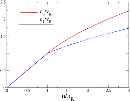
Figure 1: (Color online). Zero-sound and first-sound velocities of the uniform 2D quasi-ideal Fermi gas with Rashba spin-orbit coupling. Solid line: scaled zero-sound velocity $c_{0}/v_{R}$ as a function of the scaled number density $n/n_{R}$. Dashed line: scaled first-sound velocity $c_{0}/v_{R}$ as a function of the scaled number density $n/n_{R}$. Here $\epsilon_{R}=mv_{R}^{2}/2$ is the Rashba energy and $n_{R}=2m\epsilon_{R}/(\pi\hbar^{2})$ is the critical Rashba density, with $v_{R}$ the Rashba coupling (Rashba velocity).

Up to now we have analyzed a two-spin-component 2D Fermi gas with spin-orbit coupling, but we have neglected the effect of the s-wave scattering length $a_{s}$ between atoms in the equation of state. This assumption of “quasi-ideal gas with spin-orbit” is reliable under the condition

$$g_{2D}\,n\ll\mu\;,$$ (13)

where $g_{2D}$ is the 2D effective interaction strength given by $4\pi\hbar^{2}a_{s}/(ma_{z}\sqrt{2\pi})$ with $a_{z}$ the characteristic length of axial harmonic confinement, while the chemical potential $\mu$ is given by Eq. (11). Thus, if Eq. (13) holds the effect of interaction can be neglected in the zero-temperature equation of state $\mu=\mu(n)$. Nevertheless, also under the condition (13) the s-wave scattering length $a_{s}$ is very important because it determines the collisional time $\tau_{c}$ of the system, given by

$$\tau_{c}={1\over n_{3D}\,\sigma\,v_{F}}\;,$$ (14)

where $n_{3D}=n/(a_{z}\sqrt{2\pi})$ is the 3D number density, $\sigma=4\pi a_{s}^{2}$ is the scattering length and $v_{F}$ is the 2D Fermi velocity, a density wave propagates with a dispersion relation

$$\omega=c_{s}\,q$$ (15)

with $\omega$ the frequency of oscillation, $q$ the wavenumber and $c_{s}$ the speed of sound.

In the collisionless regime, where $\omega\tau_{c}\gg 1$, the sound is called zero sound and the corresponding zero-sound velocity $c_{s}=c_{0}$ is given by the Landau formula sala-fermi-reduce ; lipparini

$$c_{0}=\sqrt{2\mu\over m}\;.$$ (16)

By using Eq. (11) we immediately find

$${c_{0}\over v_{R}}=\left\{\begin{array}[]{ccc}{n\over n_{R}}&\mbox{for}&0\leq n<n_{R}\\ \sqrt{-1+2{n\over n_{R}}}&\mbox{for}&n\geq n_{R}\end{array}\right.\;,$$ (17)

where $v_{R}=\sqrt{2\epsilon_{R}/m}$ is the Rashba velocity with $\epsilon_{R}=mv_{R}^{2}/2=\pi\hbar^{2}n_{R}/(2m)$ the Rashba energy. Notice that, according to our definitions, $v_{R}/v_{F}=\sqrt{n_{R}/(2n)}$. Moreover, in the absence of spin-orbit coupling, i.e. for $v_{R}=\epsilon_{R}=n_{R}=0$, the 2D zero-sound velocity $c_{0}$ becomes the 2D zero-sound velocity of the 2D ideal Fermi gas, which is nothing else than the 2D Fermi velocity $v_{F}=\sqrt{2\pi\hbar^{2}n/m^{2}}$.

In the collisional regime, where $\omega\tau_{c}\ll 1$, the sound is called first sound and the corresponding first-sound velocity $c_{s}=c_{1}$ is given by the thermodynamics formula sala-fermi-reduce ; lipparini

$$c_{1}=\sqrt{{n\over m}{\partial\mu\over\partial n}}\;.$$ (18)

By using Eq. (11) we immediately find

$${c_{1}\over v_{R}}=\left\{\begin{array}[]{ccc}{n\over n_{R}}&\mbox{for}&0\leq n<n_{R}\\ \sqrt{n\over n_{R}}&\mbox{for}&n\geq n_{R}\end{array}\right.\;.$$ (19)

Notice that, in general, for a uniform superfluid the first sound velocity can be obtained either by Eq. (18) or from a detailed calculation of vertex function (i.e. within Random Phase Approximation). These two may be considered as macroscopic and microscopic sound velocity, respectively. In the spin-orbit coupled system, the Galilean invariance is broken and the macroscopic and microscopic sound velocities could be different: we are presently working on this puzzling issue. From Eq. (19) one finds that, in the absence of spin-orbit coupling, i.e. for $v_{R}=\epsilon_{R}=n_{R}=0$, the 2D first-sound velocity $c_{1}$ becomes the 2D first-sound velocity of the 2D ideal Fermi gas, namely $c_{1}=v_{F}/\sqrt{2}$ with $v_{F}=\sqrt{2\pi\hbar^{2}n/m^{2}}$ the 2D Fermi velocity of the ideal Fermi gas.

In Fig. 1 we report both zero and first sound velocities as a function of the scaled number density $n/n_{R}$. For $n<n_{R}$ the two velocities coincide while for $n>n_{R}$ they have a different behavior. Without spin-orbit coupling, i.e. for $v_{R}=\epsilon_{R}=n_{R}=0$, it is immediate to find that $c_{0}=v_{F}$ and $c_{1}=v_{F}/\sqrt{2}$, which are the text-book results of a 2D quasi-ideal Fermi gas lipparini .

We now switch on the soft harmonic potential in the $(x,y)$ plane, i.e. we consider the case $\omega_{\bot}\neq 0$ in Eq. (2). Within the local density (Thomas-Fermi) approximation lipparini we perform the following shift in the 2D chemical potential

$$\mu\to\mu-{1\over 2}m\omega_{\bot}r^{2}\;,$$ (20)

where $r=\sqrt{x^{2}+y^{2}}$ is the cylindric radial coordinate. By using Eq. (20) into Eq. (11) we obtain the 2D local number density $n(r)$, which is the density profile of fermionic cloud.

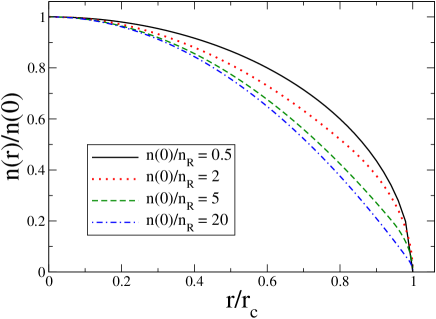
Figure 2: (Color online). Radial density profile $n(r)$ of the uniform 2D quasi-ideal Fermi gas with Rashba spin-orbit coupling in a harmonic trap. The four curves correspond to different values of the ratio $n(0)/n_{R}$ where $n(0)$ is the 2D local density at the center of the cloud and $n_{R}=m^{2}v_{R}^{2}/(\pi\hbar^{2})$ is the characteristic Rashba density, with $v_{R}$ the Rashba coupling (Rashba velocity).

It is not difficult to show that the density profile crucially depends on its value $n(0)$ at the center of the harmonic trap. In particular, if $n(0)<n_{R}$ we find

$$n(r)=n(0)\sqrt{1-{r^{2}\over r_{c}^{2}}}\quad\mbox{for}\quad 0\leq r\leq r_{c}\;,$$ (21)

where $r_{c}=r_{R}(n(0)/n_{R})$ is the critical radius such that $n(r_{c})=0$, and $r_{R}=\sqrt{2\epsilon_{R}/(m\omega_{\bot})}$ is the Rashba radius with $\epsilon_{R}=\pi\hbar^{2}n_{R}/(2m)$. Obviously, in this case $r_{c}<r_{R}$. Instead, if $n(0)>n_{R}$ we obtain

$$n(r)=\left\{\begin{array}[]{ccc}n(0)\big{(}1-{r^{2}\over r_{b}^{2}}\big{)}&\mbox{for}&0\leq r<r_{0}\\ n(0){1-{r_{0}^{2}\over r_{1}^{2}}\over\sqrt{1-{r_{0}^{2}\over r_{c}^{2}}}}\sqrt{1-{r^{2}\over r_{c}^{2}}}&\mbox{for}&r_{0}\leq r\leq r_{c}\end{array}\right.\;,$$ (22)

where $r_{0}=r_{R}\sqrt{2(n(0)/n_{R})-2}$, $r_{1}=r_{R}\sqrt{2(n(0)/n_{R})}$, and $r_{c}=r_{R}\sqrt{2(n(0)/n_{R})-1}$. Again $r_{R}=\sqrt{2\epsilon_{R}/(m\omega_{\bot})}$ is the Rashba radius and moreover $r_{0}<r_{R}<r_{c}<r_{1}$. In Fig. 2 we report the radial density profile $n(r)$ for four diffeent values of the ratio $n(0)/n_{R}$. We actually plot the scaled radial density $n(r)/n(0)$ as a function of the scaled cylindric radius $r/r_{c}$, such that both $n(r)/n(0)$ and $r/r_{c}$ are confined in the interval $[0,1]$. Notice that the solid curve obtained with $n(0)/n_{R}=0.5$ is indeed the same for any ratio $n(0)/n_{R}$ between $0$ and $1$. Instead for $n(0)/n_{R}>1$ our scaled density profile depends on the chosen ratio, as shown in the figure.

In conclusion, we have shown that the inclusion of a Rashba spin-orbit coupling in a quasi-ideal 2D Fermi gas implies the existence of a critical Rashba density, which depends on the Rashba coupling strength, at which the equation of state and other physical properties, e.g. speed of sound and density profiles, drastically change. Indeed at this critical Rashba density there is a third-order phase transition, because, as shown by Eq. (11), the second derivative of the chemical potential $\mu$ with respect to the number density $n$ has a jump at the critical Rashba density $n_{R}$. We believe our predictions can be experimentally tested with the available setups.

References

- (1) Y. J. Lin, K. Jimenez-Garcia, and I. B. Spielman, Nature 471, 83 (2011).
- (2) J.-Y. Zhang, S.-C. Ji, Z. Chen, L. Zhang, Z.-D. Du, B. Yan, G.-S. Pan, B. Zhao, Y.-J. Deng, H. Zhai, S. Chen, and J.-W. Pan, Phys. Rev. Lett. 109, 115301 (2012).
- (3) P. Wang, Z.-Q. Yu, Z. Fu, J. Miao, L. Huang, S. Chai, H. Zhai, and J. Zhang, Phys. Rev. Lett. 109, 095301 (2012).
- (4) L. W. Cheuk, A. T. Sommer, Z. Hadzibabic, T. Yefsah, W. S. Bakr, and M. W. Zwierlein, Phys. Rev. Lett. 109, 095302 (2012).
- (5) Y.A. Bychkov and E.I. Rashba, J. Phys. C 17, 6029 (1984).
- (6) G. Dresselhaus, Phys. Rev. 100, 580 (1955).
- (7) Y. Li, L.P. Pitaevskii, and S. Stringari, Phys. Rev. Lett. 108, 225301 (2012).
- (8) G.I. Martone, Yun Li, P.L. Pitaevskii, and S. Stringari, Phys. Rev. A 86, 063621 (2012).
- (9) M. Burrello and A. Trombettoni, Phys. Rev. A 84, 043625 (2011).
- (10) M. Merk, A. Jacob, F. E. Zimmer, P. Ohberg, and L. Santos, Phys. Rev. Lett. 104, 073603 (2010); O. Fialko, J. Brand, and U. Zuelicke, Phys. Rev. A 85, 051605 (2012); R. Liao, Z.-G. Huang, X.-M. Lin, and W.-M. Liu, ibid. 87, 043605 (2013).
- (11) V. Achilleos, D. J. Frantzeskakis, P. G. Kevrekidis, and D. E. Pelinovsky, e-preprint arXiv:1211.0199.
- (12) Y. Xu, Y. Zhang, and B. Wu, Phys. Rev. A 87, 013614 (2013).
- (13) L. Salasnich and B.A. Malomed, Phys. Rev. A 87, 063625 (2013).
- (14) X.-Q. Xu and J. H. Han, Phys. Rev. Lett. 107, 200401 (2011); S. Sinha, R. Nath, and L. Santos, Phys. Rev. Lett. 107, 270401(2011); C.-F. Liu and W. M. Liu, Phys. Rev. A 86, 033602 (2012); E. Ruokokoski, J. A. Huhtamaki, and M. Mottonen, Phys. Rev. A 86, 051607 (2012); H. Sakaguchi, and B. Li, Phys. Rev. A 87, 015602 (2013).
- (15) Y. Deng, J. Cheng, H. Jing, C. P. Sun, and S. Yi, Phys. Rev. Lett. 108, 125301 (2012).
- (16) J. P. Vyasanakere and V. B. Shenoy, Phys. Rev. B 83, 094515 (2011).
- (17) J. P. Vyasanakere, S. Zhang, and V. B. Shenoy, Phys. Rev. B 84, 014512 (2011).
- (18) M. Gong, S. Tewari, and C. Zhang, Phys. Rev. Lett. 107, 195303 (2011).
- (19) H. Hu, L. Jiang, X-J. Liu, and H. Pu, Phys. Rev. Lett. 107, 195304 (2011).
- (20) Z-Q. Yu and H. Zhai, Phys. Rev. Lett. 107, 195305 (2011).
- (21) M. Iskin and A. L. Subasi, Phys. Rev. Lett. 107, 050402 (2011).
- (22) W. Yi and G.-C. Guo, Phys. Rev. A 84, 031608 (2011).
- (23) L. Dell’Anna, G. Mazzarella, and L. Salasnich, Phys. Rev. A 84, 033633 (2011).
- (24) M. Iskin and A. L. Subasi, Phys. Rev. A 84, 043621 (2011).
- (25) J. Zhou, W. Zhang, and W. Yi, Phys. Rev. A, 84, 063603 (2011).
- (26) L. Jiang, X.-J. Liu, H. Hu, and H. Pu, Phys. Rev. A 84, 063618 (2011).
- (27) Li Han and C.A.R. Sa de Melo, Phys. Rev. A 85, 011606(R) (2012).
- (28) G. Chen, M. Gong, and C. Zhang, Phys. Rev. A 85, 013601 (2012)
- (29) K. Zhou, Z. Zhang, Phys. Rev. Lett. 108, 025301 (2012).
- (30) X. Yang, S. Wan, Phys. Rev. A 85, 023633 (2012)
- (31) M. Iskin, Phys. Rev. A 85, 013622 (2012).
- (32) K. Seo, L. Han, C.A.R. Sa de Melo, Phys. Rev. A 85, 033601 (2012).
- (33) L. He and Xu-Guang Huang, Phys. Rev. Lett. 108, 145302 (2012).
- (34) X.J. Liu et al., Phys. Rev. Lett. 102, 046402 (2009).
- (35) P. Wang et al., Phys. Rev. Lett. 109, 095301 (2012).
- (36) L.W. Cheuk et al., Phys. Rev. Lett. 109, 095302 (2012).
- (37) L. Salasnich and F. Toigo, J. Low Temp. Phys. 150, 643 (2008); G. Mazzarella, L. Salasnich, and F. Toigo, Phys. Rev. A 79, 023615 (2009).
- (38) E. Lipparini, Modern Many-Particle Physics - 2nd edition (World Scientific, Singapore, 2008).
- (39) H. Hu and X.-J. Liu, Phys. Rev. A 85, 013619 (2012).
- (40) K. Huang, Statistical Mechanics (Wiley, New York, 1987); S. Sachdev, Quantum Phase Transitions (Cambridge Univ. Press, Cambridge, 2011).