Relativistic AGN jets II. Jet properties and mixing effects for episodic jet activity

Abstract

Various radio galaxies show signs of having gone through episodic jet outbursts in the past. An example is the class of double-double radio galaxies (DDRGs). However, to follow the evolution of an individual source in real-time is impossible due to the large time scales involved. Numerical studies provide a powerful tool to investigate the temporal behavior of episodic jet outbursts in a (magneto-)hydrodynamical setting. We simulate the injection of two jets from active galactic nuclei (AGN), separated by a short interruption time. Three different jet models are compared. We find that an AGN jet outburst cycle can be divided into four phases. The most prominent phase occurs when the restarted jet is propagating completely inside the hot and inflated cocoon left behind by the initial jet. In that case, the jet-head advance speed of the restarted jet is significantly higher than the initial jet-head. While the head of the initial jet interacts strongly with the ambient medium, the restarted jet propagates almost unimpeded. As a result, the restarted jet maintains a strong radial integrity. Just a very small fraction of the amount of shocked jet material flows back through the cocoon compared to that of the initial jet and much weaker shocks are found at the head of the restarted jet. We find that the features of the restarted jet in this phase closely resemble the observed properties of a typical DDRG.

1 Introduction

Over the last decade, a new class of radio sources called Double-Double Radio Galaxies (DDRGs) has been identified (e.g. Schoenmakers et al. 2000; Saikia & Jamrozy 2009). These sources can be characterized by a pair of double hotspots and/or radio lobes driven by the same SMBH. Some rare examples have even been reported where three distinct pairs of radio lobes are seen on both sides of the AGN. In that case the source is referred to as a Triple-Double Radio Galaxy (e.g. Hota et al., 2011). Figure 1 shows the radio map for the source PKS B1545-321 (B1545-321 hereafter), a typical example of a DDRG (Saripalli, Subrahmanyan & Udaya Shankar (2003); Safouris et al. (2008)). Of the (roughly 20) DDRGs that are known to date, the distance of the inner radio lobes to the central engine range from as close as 14 pc as in J1247+6723 (Saikia, Gupta & Konar, 2007), up to several hundreds of kpc as in J1835+6024 (Lara et al., 1999). The distance of the outer lobes to the central engine is usually much larger, of the order of a few Mpc.

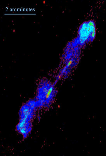
Figure 1: Non-thermal (synchrotron) radio emission of the Double-Double Radio Galaxy PKS B1545-321, observed at 1384 MHz and 2496 MHz with the ATCA. Two prominent outer radio lobes and two less prominent inner lobes are visible. The total size of the source is $\sim$ 1 Mpc. The North-East part of the source is pointed away from the observer. Credits: Saripalli et al. (2003).

Jet properties such as stability and the integrity of the transverse (radial) structure, the impact of the jet on the intergalactic medium (IGM) and the closely related jet-head advance speed depend strongly on the properties of the ambient medium through which the jets propagate. If an AGN undergoes multiple cycles of activity, it is capable of drastically changing this ambient medium. Multiple pairs of radio lobes and hotspots within the same radio galaxy are strong indications for the occurrence of episodic jet eruptions in AGNs (see for example Saripalli et al. 2003; Safouris et al. 2008; Konar & Hardcastle 013a; Konar et al. 013b; Konar et al. 013c; Konar et al. 013d). In some cases the interruption time, that is the time between two subsequent jet eruptions, for DDRGs is short compared to the duration of the initial jet eruption, as recent studies suggest (Konar et al. 013b; Konar et al. 013c). Then, the signatures from both eruptions (mainly in the form of synchrotron radiation) are observed simultaneously. However, if the interruption time is comparable with, or larger than the duration of the initial jet eruption, the inflated hot cocoon (a mixture of shocked IGM and shocked jet material, hereafter ‘dIGM’) from the first eruption has the chance to expand and the non-thermal electrons have the chance to cool significantly before the next eruption begins. In that case, the radiation from the relativistic leptons produced in the initial jet eruption might no longer be observable, whereas the conditions of the disturbed medium still significantly differ from those of the undisturbed ambient medium (hereafter ‘uIGM’). Having a better understanding of episodic AGN jet activity, the time scales involved and the effect of episodic outbursts on the ambient medium will contribute to a more global understanding of AGN jets and galaxy evolution in general.

There are a number of reasons for studying episodic AGN jet behavior. For an AGN that launches a jet into an uIGM, jet properties (such as jet-head advance speed, stability and transverse structural integrity, or the dynamics of the hotspots, cocoon and back-flow of shocked jet material), are expected to be quite different from jets in a source that shows multiple outbursts. This is even true when the intrinsic characteristics such as power, the direction into which the jet is injected, opening angle, injection spectral index, etc. are equal. It is impossible to directly follow AGN jet eruption cycles due to the enormous length/time scales involved (up to hundreds of Myr, see for example McNamara & Nulsen 2007; Wise et al. 2007 or McNamara & Nulsen 2012). Therefore, observational evidence for the existence of episodic AGN jet cycles in an individual source can only indirectly be inferred from synchrotron spectral ages and morphology, such as the distances of different synchrotron-emitting regions to the central engine. Fortunately, hydrodynamical (HD) simulations of relativistic AGN jets provide a tool for calculating the (strong non-linear) large-scale behavior of these jet flows and their surrounding ambient medium, offering a powerful method to ultimately help model the observations. The aim is then to identify the characteristic features that are seen in the different phases of a jet outburst in the simulation and compare them with the observed signatures in the emitted non-thermal radiation from such a radio source.

Numerical studies that are related to time-dependent/episodic jet behavior go back to the study of Wilson (1984) who simulates jets with a sinusoidally varying jet speed. Clarke & Burns (1991) simulate restarting 2-dimensional magnetohydrodynamic (2D MHD) non-relativistic jets. In powerful radio galaxies where jets show typical Lorentz factors of a few up to $\sim 50$, relativistic effects need to be taken into account in order to simulate a realistic scenario. Chon et al. (2012) perform a 3D HD simulation of a restarting jet in the FRII radio galaxy Cygnus A. Their paper focusses on an X-ray cavity observed near the parent galaxy of the radio source Cygnus A that is believed to be created by a jet event that took place ∼ 30 Myr ago. By simulating the X-ray emission at a late time during the second jet eruption, they find that the regions containing jet material from the first eruption show up as X-ray cavities, similar to those observed in Cygnus A. Although a relevant case study for Cygnus A, the intermediate phases leading to its current state, as well as the jet dynamics itself are not treated. Finally Mendygral, Jones & Dolag (2012) study restarting 3D non-relativistic MHD jets injected into the external medium of a galaxy cluster to investigate the influence of this intra-cluster medium (ICM) on the morphological evolution of the jets and their radio lobes. These simulations mainly probe the large-scale characteristics of the resulting radio lobes and X-ray cavities.

All these studies consider non-relativistic jets that are homogeneous in the radial direction. An exception is the work of Mendygral et al. 2012, who include a radially varying electromagnetic field. However, AGN jets show strong signs of stratification transverse to their direction of propagation (i.e. radial stratification). The observations favor a jet consisting of a low-density and fast-moving spine, surrounded by a denser and slower moving region called the jet sheath (see for example Sol, Pelletier & Asseo 1989; Giroletti et al. 2004; Ghisellini, Tavecchio & Chiaberge 2005; Gómez et al. 2008). In Walg et al. (2013), hereafter SW1, we presented the study of the evolution of relativistic axisymmetric jets with three different transverse jet profiles carrying angular momentum, for a steady jet driven by a continuous inflow.

2 Main focus of this research

We present the first special relativistic simulations of episodic outbursts of AGN jets. These simulations allow us to accurately study the jet dynamics, as well as the amount of shocked back-flowing jet material at the jet-head. To that end, we simulate two distinct episodes of jet activity. We keep track of the constituents of both jets. The aim here is to understand the processes that lead to the morphology of a DDRG such as B1545-321. In the follow-up paper, these same simulations will be used to study synchrotron emission at the various stages of an episodic jet event. Our choice of parameters is representative for a typical powerful radio galaxy and is representative for a typical DDRG. We will focus on the following points:

• How does jet stratification change during an activity cycle;

• How does the propagation of the restarted jet in the cycle differ from the first jet, and what determines the jet-head advance speed;

• How rapidly do the strong shocks at the jet-head fade after the first jet has been turned off;

• How does mixing between the different constituents (ambient medium, spine material, sheath material) take place and how is the amount of mixing influenced by episodic activity. In particular: to what amount does material from the first and the second jet mix.

All these features that follow from the simulations will add to our understanding and interpretation of the rich diversity and large-scale structures that are observed in giant radio galaxies, such as DDRGs.

The outline of this paper is as follows: in Section 3 we present the background theory. In Section 4 we discuss the method, numerical schemes and the parameter regime. In Section 5 we describe the different simulations and their results. Discussion and Conclusions can be found in Sections 6 and 7.

3 Theoretical background

3.1 Relation between the DDRG synchrotron emission and the dynamics of the jet flow

The intensity of the synchrotron emission that is emitted from an extragalactic radio source (at a certain acceleration site) depends on [1] the rate of injection of relativistic particles, [2] the frequency $\nu$ at which the source is observed and [3] the synchrotron cooling time $\tau_{\rm synchro}(\nu)$ at that frequency. In addition, adiabatic cooling due to source expansion affects the synchrotron intensity at all frequencies. The time-scale for adiabatic cooling, $\tau_{hydro}$, is closely related to the hydrodynamical properties (and time-scales) of the gas. There are two limiting cases, namely:

$\tau_{\rm hydro}\gg\tau_{\rm synchro}$, in which case the energy losses are dominated by the synchrotron cooling;

$\tau_{\rm hydro}\ll\tau_{\rm synchro}$, in which case the energy losses are dominated by the adiabatic cooling (expansion losses).

In this paper, the dynamical time scales, such as duration of the active outbursts phases or the interruption times, are $\sim 10^{6}-10^{7}$ yr. These time-scales are short compared to the synchrotron cooling time at radio frequencies of $\sim 1-2$ GHz, which are typical frequencies at which DDRGs are observed (see for example Harwood et al. 2013). Therefore, the energy losses of the electrons responsible for the synchrotron emission for the radio galaxies that we are considering are dominated by the effect of the expansion of the gas.

A typical DDRG is believed to be the result of a restarting jet propagating inside a disturbed medium dIGM of an earlier eruption that took place a relatively short time ago (interruption time much less than lifetime of an individual jet). Moreover, since the radio lobes and/or hotspots of the initial jet eruption are still visible, either the outer radio lobes and hotspots are still being fed by fresh material from the initial jet (as is assumed to be the case for the DDRG J1835+6204), or the initial jet has disappeared very recently as is believed to be the case for B1545-321. We will consider a similar situation for the jet models in this paper. We will follow the restarting jet up to and including the propagation outside of the initial cocoon, in the uIGM.

Table 1: List of computer normalization units (or characteristic quantities) that we chose for these simulations in cgs units. These characteristic quantities are the same as in SW1 and apply throughout this paper.

Char. quantities	symbol	cgs units
Number density	$n_{\rm ch}$	$10^{-3}\;{\rm cm}^{-3}$
Pressure	$P_{\rm ch}$	$1.50\times 10^{-6}\;{\rm erg\;cm}^{-3}$
Temperature	$T_{\rm ch}$	$1.09\times 10^{13}\;{\rm K}$

3.2 Outburst cycle time scales for DDRGs

The age of a radio galaxy is often inferred from the synchrotron spectral age of its radio lobes or its plumes (e.g. Harwood et al., 2013). In this way, some of the larger sources are estimated to be of the order of $10^{6}-10^{8}$ yr old (see for example Jamrozy et al. 2008; Konar et al. 2008; O’Dea et al. 2009 or Saikia & Jamrozy 2009).

Recent studies suggest that, for BH systems with an accretion rate well below the Eddington limit, $\dot{M}_{\rm BH}\ll\dot{M}_{\rm edd}$, accretion and jet formation behave in a similar fashion, scalable by BH mass. An indication for this scaling was found by McHardy et al. 2006, where they show a mass dependence of characteristic time scales for the variability of the emission produced near black holes of black hole binaries (BHBs) and AGNs. Another strong indication for mass scaling accretion physics is the observed correlation between the luminosities in X-ray and Radio frequencies for these systems. A number of authors (e.g. Corbel et al. 2000; Corbel et al. 2003; Merloni, Heinz & di Matteo 2003; Falcke, Körding & Markoff 2004; Körding, Falcke & Corbel 2006 and Plotkin et al. 2012) have studied the relationship between X-ray luminosity ($L_{\rm{X}}$), radio luminosity ($L_{\rm{R}}$) and BH mass ($M_{\rm{BH}}$) for BH systems with a low accretion rate in BHBs, as well as in SMBHs in the centre of active galaxies. They have shown a relationship between $L_{\rm{X}}$, $L_{\rm{R}}$ and $M_{\rm{BH}}$ that holds over many orders of magnitude in BH mass, ranging from stellar-mass BHs with a typical mass of $M_{\rm BH}\sim 10M_{\odot}$ up to the largest SMBHs with a typical mass of $M_{\rm BH}\sim 10^{9}M_{\odot}$. This relation defines a plane in three-dimensional $(\log L_{\rm{X}},\log L_{\rm{R}},\log M_{\rm{BH}})$ parameter space, called the fundamental plane of BH accretion.

Table 2: Global parameters of the ambient medium and the jet at the jet inlet as used in the models $H2$, $I2$, $A2$. From left to right they are: kinetic luminosity ($L_{\rm jt}$), number density ($n$), Lorentz factor ($\gamma$), azimuthal velocity ($V_{\phi}$) and polytropic index ($\Gamma$) used to setup the transverse (radial) pressure profile of the jets. In case of model $H2$, the jet is homogeneous in the transverse direction and is described by single-valued quantities. The parameters for models $I2$ and $A2$ are initialized separately for spine (denoted as ”sp” in the table) and sheath (denoted as ”sh” in the table). In case of model $I2$ and $A2$, the pressure varies smoothly in the radial direction.

Models	$L_{\rm jt}\;[10^{46}\;\mathrm{erg\;s^{-1}}]$	$n\;[10^{-6}\;\mathrm{cm^{-3}}]$	$\gamma$	$V_{\phi}\;[10^{-3}\;c]$	$\Gamma$
	sp $|$ sh	sp $|$ sh	sp $|$ sh	sp $|$ sh	sp $|$ sh
$\mathbf{H}$ (homogeneous)	3.82	4.55	3.11	0.0	1
$\mathbf{I}$ (isothermal)	1.82 3.35	$P/\rho=$ constant	6.0 3.0	1.0 1.0	5/3 5/3
$\mathbf{A}$ (constant density)	0.44 3.39	1.0 5.0	6.0 3.0	1.0 1.0	5/3 5/3
External medium	-	$1.0\times 10^{3}$	-	-	5/3

Many BHBs are observed to go through outburst cycles (e.g. Rodríguez & Mirabel 1999; Fender 2002). It is generally believed that AGNs also go through outburst cycles, but it is unclear whether these cycles are driven by the same physical mechanisms. A scenario that can explain the origin and the specific morphology of DDRGs is given by Liu, Wu & Cao (2003) who suggest an inspiraling SMBH binary as a result of two merging galaxies to be the cause. In their model, the secondary SMBH slowly sinks towards the centre of mass, causing a gap in the inner accretion disc to occur. In this way, the jet formation of the primary SMBH is temporarily stopped. When the gap is refilled by material from the outer accretion disc (on a viscous time-scale of $\sim 1$ Myr), jet formation is restarted. Cycle times for accreting SMBHs are typically long ($\sim 10^{6}-10^{8}$ yr). These large time-scales suggest that, at least in sources like DDRGs, the observed morphology of the source is essentially a snapshot of an ongoing eruption event.

4 Method

4.1 The jet models, the parameters and initial conditions

Consider a central engine in the nucleus of a radio galaxy that undergoes two or more subsequent jet eruptions. If the different episodes are triggered by the same mechanism (for example, a large in-falling gas cloud), it is reasonable to assume that the typical initial jet properties near the central engine, as for example mass density, bulk outflow velocity, rotation, etc., should be approximately similar for the subsequent jet eruptions (also see Konar & Hardcastle 013a; Konar et al. 013d). In this paper we will assume all the jet parameters to be equal for the two subsequent jet eruptions.

We employ MPI-AMRVAC (Keppens et al., 2012) and simulate the jets with a special relativistic hydrodynamical (SRHD) module. We use the spatial Harten-Lax-van Leer Contact (HLLC) solver (Toro, Spruce & Speares 1994; Mignone & Bodo 2005) for the three jet models, in combination with a three-step Runge-Kutta time-discretization scheme and a Koren limiter (Koren, 1993).

The jets are cylindrically symmetric ($2.5D$) with the $Z-$axis defined along their axis. The jet flows are created by injecting material into the computational domain through the boundary cells at the $Z=0$ axis, between $R=0$ and $R=R_{\rm jt}=$ 1 kpc, which we refer to as the jet inlet. Except for the cells involved in injecting the jet material (during the active phase of jet injection), all other cells in the lower boundary are free outflow boundaries. In case of the structured jets, we choose the radius of the spine equal to $R_{\rm s}=R_{\rm jt}/3$.

The size of the computational domain is $(120\times 480)$ kpc², comparable to the size of either one of the jets in B1545-321 (see Figure 1). The basic resolution is $(120\times 480)$ grid cells, and we allow for 3 additional refinement levels, resulting in an effective resolution of $(960\times 3840)$ grid cells. The jet is resolved by 8 grid cells across the jet radius. Therefore, we can resolve details down to $(125\times 125)$ pc².

For the polytropic index $\Gamma_{\rm eff}$ of the gas we work with the Mathews approximation for the Synge EOS of the gas (Blumenthal & Mathews, 1976). In this approximation, the gas pressure $P$ is defined by the closure relation:

$$P=\frac{1}{3}\left(e-\frac{\rho^{2}}{e}\right)\;,$$ (1)

with $e=e_{\rm th}+\rho$, the internal energy density consisting of the rest-mass density $\rho$ and thermal energy density $e_{\rm th}$. We employ units where $c=1$. This approximation gives an accurate interpolation between a classically ’cold’ gas with an adiabatic index $\Gamma_{\rm eff}=5/3$ and a relativistically ’hot’ gas with $\Gamma_{\rm eff}=4/3$. We define the transition from cold to relativistically hot to occur when the internal energy per particle is equal to the rest-mass energy per particle, i.e. $k_{\rm B}T=m_{\rm p}c^{2}$, resulting in $\Gamma_{\rm eff}=1.417$.

The jet models that are used in this paper are the same as those used in SW1. They include a transverse homogeneous jet ($H$) and two jets with a transverse spine–sheath jet structure that carry angular momentum. At the jet inlet, radial force-balance is maintained along the jet cross-section. The condition of radial force-balance, together with the azimuthal velocity profile, $v_{\phi}(R)$ determine the pressure profile, $P(R)$, across the jet cross-section. However, the azimuthal velocity at the length scales that we are considering are thought to be small compared to the poloidal velocity ($v_{\phi}\ll v_{\rm Z}$), so it has a negligible influence on the dynamics of the jets.

One jet with radial structure is set up using an isothermal equation of state ($I$), which we denote as the isothermal jet. The other uses a constant, but different density for spine and sheath ($A$), which we denote as the (piecewise) isochoric jet. To distinguish between the steady case scenario (denoted with an index ‘1’), and the episodic scenario, we refer to the models in this paper as $H2$, $I2$ and $A2$ respectively. The isochoric jet $A2$ and the isothermal jet $I2$ consist of a jet spine–sheath structure that is characterized by having a different bulk Lorentz factor for jet spine and jet sheath. The isochoric jet $A2$ is initiated and injected with a constant, but different mass density for the jet spine and the jet sheath. The isothermal jet $I2$ is initiated and injected with a constant temperature across the entire cross-section.

The jet models are based on realistic values for mass density $\rho=m_{\rm p}n$, with $m_{\rm p}$ the proton mass, $n$ the number density and temperature $T_{\rm am}$ of a typical ICM environment (see e.g. Davé et al. 2001; Davé et al. 2010 and Kunz et al. 2011). Moreover, jet bulk Lorentz factors $\gamma_{\rm jt}$ are used that are typical for jets driven by SMBHs at these length scales. The density ratio $\eta_{\rm R}=n_{\rm jt}/n_{\rm am}$ between the jet and the ICM are deduced from the jet luminosity $L_{\rm jt}$. In the initial setup, all jets are in pressure equilibrium with their surrounding at the interface between the jet and the ambient medium. Tables 1 and 2 show the parameters used in these models. For a detailed discussion on the set up of the radial jet profiles, we refer the reader to SW1.

4.2 Quantifying mixing for multiple constituents

We employ tracers, $\theta_{\rm A}(t,\mn@boldsymbol{r})$, that are passively advected by the flow from cell to cell in the numerical grid employed in the simulations. We initiate them as follows:

H2: for the homogeneous jet with two eruptions we use two tracers $\theta_{i}$, with $i=1$ for the material involved in the initial jet eruption and $i=2$ for the subsequent one. Jet material is initialized as $\theta_{i}=+1$ and ambient medium material as $\theta_{i}=0$.

A2 and I2: these models simulate the case of episodic jets with a transverse spine–sheath structure. For these jets we use four tracers, $\{\theta_{i}^{\rm sp},\theta_{i}^{\rm sh}\}$, with again $i=1$ for material involved in the initial eruption and $i=2$ for the subsequent one. The tracers $\theta_{i}^{\rm sp}$ are initialized as +1 for spine material and as 0 elsewhere. Equivalently, the tracers $\theta_{i}^{\rm sh}$ are initialized as +1 for sheath material and 0 elsewhere .

We will interpret the tracer value $\theta_{\rm A}(t,\mn@boldsymbol{r})$ in a certain grid cell to be equal to the mass fraction $\delta_{\rm A}(t,\mn@boldsymbol{r})$ of constituent $A$ in that grid cell (and similar for constituent $B$).

In SW1, we performed a quantitative analysis of mixing. We introduced two practical mixing quantities, the first called absolute mixing, denoted as $\Delta$ and the second called mass-weighted mixing, denoted as $\Lambda$. These two quantities can compactly be written as:

$$\mathcal{M}_{\rm J}=1-\left|\frac{\delta_{\rm A}-\mu_{\rm J}\delta_{\rm B}}{\delta_{\rm A}+\mu_{\rm J}\delta_{\rm B}}\right|\;,$$ (2)

with $\mathcal{M}_{\rm J}=\{\Delta,\Lambda\}$ the absolute mixing and mass-weighted mixing respectively, where we dropped the notation for the time- and space dependence, $(t,\mn@boldsymbol{r})$. Moreover, $\mu_{\rm J}=\{1,M_{\rm A}/M_{\rm B}\}$, with $M_{\rm A}$ and $M_{\rm B}$ the total masses of constituents $A$ and $B$ contained in the total computational volume respectively. With this definition for the amount of mixing, $\mathcal{M}_{\rm J}=0$ means the constituents $A$ and $B$ have not mixed at all, whereas $\mathcal{M}_{\rm J}=1$ means the constituents have fully mixed. We refer the reader to SW1 for a more detailed discussion on tracer advection and mixing.

4.3 Time scales of the various phases of the jet eruptions

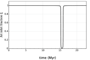
Figure 2: Jet inlet fraction showing the activity of the central engine that is driving the jets. The poloidal velocity of the jets $v_{z}(t)$ is determined by $v_{z}=\xi(t)\times V_{z}$, where the parameter $V_{z}$ is a fixed number and follows from the Lorentz factor of that jet component. At $t$ = 15.3 Myr, the central engine switches off and at $t$ = 16.0 Myr, a subsequent jet is injected into the system for another 6.8 Myr. The simulation is stopped at $t$ = 22.8 Myr.

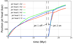
Figure 3: Jet-head propagation for two subsequent episodic jet outbursts for models $A2$, $H2$ and $I2$. As with the jet models in SW1, the initial jets show a start-up phase of $\sim 3$ Myr, where the jet-head advance speed is slightly larger than after that phase. At $t$ = 15.3 Myr, the initial jets are switched off. However, the left-over jet continues to propagate towards the termination shock. At $t$ = 16.0 Myr, a restarting jet is injected into the system. It propagates significantly faster through the remnant cocoon, until it hits the edge of the remnant cocoon. At that point, it continues to propagate in the same fashion as the initial jets.

The age of a typical DDRG is estimated to be of the order of $10^{7}-10^{8}$ yr with a total length of $\sim 1$ Mpc, as for example in the case of B1545-321 (see Safouris et al. 2008). Moreover, the interruption time between the two jet events is usually short, only a few percent of the duration of the first jet eruption. In the simulations in this paper, we choose a similar setup, but consider a length/time scale that is roughly a factor of 2 smaller than that of B1545-321. Choosing the total simulation time equal to that in SW1 ($t_{\rm tot}=22.8$ Myr) [1] allows for a fair comparison between the two studies, [2] captures the general behavior of an episodic AGN jet event and [3] does not exhaust computational resources. In order for the initial jet/cocoon to reach a typical length of a few hundred kpc, we take the initial eruption time $t_{\rm jet_{1}}=15.3$ Myr ( = $2/3\times t_{\rm tot}$). Then we choose an interruption time of $t_{\rm int}=0.045\times t_{\rm jet_{1}}=0.68$ Myr. With this choice, we find that the length of the restarted jet is approximately 1/3 of the cocoon at the moment that the first jet disappears, in agreement with the morphology of B1545-321 (see Figure 1). Finally, we inject the second jet for the remaining $t_{\rm jet_{2}}=6.8$ Myr. We stop the simulations at the point where the second jet-head has completely traversed the dIGM, so that the front end of the jet is propagating in the uIGM, but before the jet runs out of the computational domain.

In order to model a smoothly varying injection of jet material at the jet inlet, we introduce a time-dependent poloidal jet bulk velocity $v_{z}(t)$ by multiplying the axial velocity $V_{z}$ with the jet inlet fraction $\xi(t)$, so that at a given time: $v_{z}(t)=\xi(t)\times V_{z}$. The jet inlet fraction $\xi(t)$ is plotted in Figure 2. For $\xi(t)$ we use the following form:

$$\xi(t)=\left\{\begin{array}[]{ll}\tau_{1}(t)+1-\tau_{1}(t=t_{0})&\mbox{for}\;t\leq t_{\rm c}\\ \tau_{2}(t)+1-\tau_{1}(t=t_{\rm tot})&\mbox{for}\;t>t_{\rm c}\;,\end{array}\right.$$ (3)

with $t$ in Myr. Here $t_{\rm tot}$ is defined above, $t_{0}=0$ is the starting time of the simulation $t_{\rm c}=t_{\rm jet_{1}}+t_{\rm int}/2$ is the time exactly halfway between the end of the first jet eruption and the beginning of the second jet eruption and the function $\tau_{k}(t)$ (with $k=\{1,2\}$) is defined as:

$$\tau_{k}(t)=\frac{1}{2}-\frac{1}{\pi}\times\arctan\left[\left(-1\right)^{k+1}\frac{\zeta}{t_{\rm tot}}\times\left(t-t_{\rm jet_{k}}\right)\right]\;.$$ (4)

We find that $\zeta=2744$ results in a fairly steep decline and rise of the jet inlet function near $t=t_{\rm jet_{1}}$ and $t=t_{\rm jet_{2}}$, while at the same time the temporal behavior of the jets is well resolved.

5 Results: stages in the evolution of a DDRG

5.1 Phase 1: the initial jet

Table 3: Jet-head advance speed $\beta_{\rm hd}$ and effective impact radius $R_{\rm am}$ [kpc] for the four different phases in episodic jet eruption. The results in phase 3 (the restarted jet propagating entirely within the remnant cocoon) differ significantly from those in the phases 1, 2 and 4.

	Phase	H2	I2	A2
$\beta_{\rm hd}$ (jet 1)	1	0.042	0.046	0.044
$\beta_{\rm hd}$ (jet 1)	2	0.031	0.052	0.037
$\beta_{\rm hd}$ (jet 2)	3	0.703	0.732	0.701
$\beta_{\rm hd}$ (jet 2)	4	0.040	0.038	0.036
$R_{\rm am}$ (jet 1)	1	4.55	4.07	4.32
$R_{\rm am}$ (jet 1)	2	6.11	3.58	5.20
$R_{\rm am}$ (jet 2)	3	1.08	0.91	1.09
$R_{\rm am}$ (jet 2)	4	4.78	4.99	5.33

In phase 1 the first jet propagates through the uIGM, the same situation as treated in detail SW1. This phase lasts approximately 15.3 Myr. We will summarize the phase 1 results briefly, and refer to SW1 for more details.

5.1.1 Jet-head advance speed

All our jets are under-dense, with a proper density ratio between jet and surrounding medium roughly equal to $\eta_{\rm R}=\rho_{\rm jt}/\rho_{\rm am}\sim 4.5\times 10^{-3}$. In such a situation the jet-head advances into the ambient medium with a speed $\beta_{\rm hd}\ll\beta_{\rm jt}$, where $\beta_{\rm hd}$ and $\beta_{\rm jt}$ are the jet-head advance speed and the bulk speed of the jet material respectively in units of $c$ in the frame where the uIGM is at rest. The jets develop significant structure (long-lived vortices) that move with the jet-head, and therefore present an obstacle for the incoming uIGM, as seen by an observer moving with the jet-head. As a result, the jet-head has an effective area $A_{\rm am}\equiv\pi\>R_{\rm am}^{2}$ perpendicular to the jet flow that is significantly larger than the geometrical cross section $A_{\rm jt}=\pi\>R_{\rm jt}^{2}$ of the undisturbed jet. Typically we find that $A_{\rm am}\simeq(16-20)\times R_{\rm jt}$. The increased effective area determines the jet-head advance speed. The relation between $\beta_{\rm hd}$, $\eta_{\rm R}$, $R_{\rm am}$ and $R_{\rm jt}$ is (SW1, Eqn. 58):

$$\beta_{\rm hd}=\frac{\displaystyle\sqrt{\eta_{\rm R}}\>\gamma_{\rm jt}\beta_{\rm jt}}{\displaystyle\Omega+\sqrt{\eta_{\rm R}}\>\gamma_{\rm jt}}\;,$$ (5)

with $\Omega\equiv R_{\rm am}/R_{\rm jt}$. Figure 3 shows the jet-head advance speed for all three models, and covers the entire simulation. In phase 1 we find similar values for the advance speed between 10 Myr and 15 Myr, when the advance is more-or-less steady. Small differences between these simulations and those of SW1 result from our use of a different solver (HLLC instead of TVDLF).

By looking carefully at the simulations we find (as in SW1) that the effective radius $R_{\rm am}$ also roughly corresponds with the transverse size of the hotspots, i.e. the region containing relativistically hot gas that has gone through the Mach disc, the strong shock that effectively terminates the high-Mach number jet flow.

Table 4: This table shows the relativistic Mach numbers ($\mathcal{M}$) for both the Mach disc (MD) and the bow shock (BS) at the jet-head for each of the three jet models $H2$, $I2$, $A2$, in phase 1 and phase 3. Moreover, the ratio of the shock strength in phase 1 and phase 3 is given for the Mach disc, as well as for the bow shock.

	Phase	H2	I2	A2
$\mathcal{M}_{\rm MD_{1}}$	1	13.3	21.7	13.2
$\mathcal{M}_{\rm MD_{2}}$	3	10.9	15.7	7.58
$\mathcal{M}_{\rm MD_{1}}/\mathcal{M}_{\rm MD_{2}}$		1.22	1.38	1.74
$\mathcal{M}_{\rm BS_{1}}$	1	32.6	35.7	34.1
$\mathcal{M}_{\rm BS_{2}}$	3	2.21	2.40	2.20
$\mathcal{M}_{\rm BS_{1}}/\mathcal{M}_{\rm BS_{2}}$		14.7	14.8	15.5

5.1.2 Temporal behavior along the jet axis

Figure 4 shows a cut along the $Z-$axis of a number of hydrodynamical quantities as a function of time. In these plots, phase 1 of the episodic jet event is contained between the left boundary of the panels and the first dashed line at $t=15.3$ Myr. The left column shows the plots for the isochoric jet $A2$ and the right column shows the plots for the isothermal jet $I2$. The pressure panels (top row) show an adjustment shock close to the jet inlet with an approximate constant distance to the jet inlet. Directly after the adjustment shock, the pressure in the jet increases significantly and shows large fluctuations (internal shocks) along the jet axis. At the jet-head (corresponding to the inclining line at the top of the disturbed regions), the hotspots can be recognized by the strong increase in pressure, as denoted by the red dots. The second row (effective polytropic index $\Gamma_{\rm eff}$) shows similar behavior: near the jet inlet the jet plasma is non-relativistically cold with $\Gamma_{\rm eff}\approx 5/3$. Nearing the jet-head, the gas becomes hotter and at the jet-head the gas is shocked to (near-)relativistic temperatures with $\Gamma_{\rm eff}\lesssim 1.417$. Finally, the third row and the bottom row show the tracer values of jet-spine and jet-sheath of the first jet. The difference in transverse structural integrity is well reflected in these plots: for the isochoric jet, immediately after the adjustment shock jet-spine material mixes with material of the jet-sheath and transverse structure is lost. However, in case of the isothermal jet, the jet-spine tracer abundance is nearly unaffected as material flows towards the jet-head.

$\begin{array}[]{c c}\includegraphics[clip={false},trim=0.0pt 0.0pt 0.0pt 0.0pt,width=195.12767pt]{fig4a.pdf}&\includegraphics[clip={false},trim=0.0pt 0.0pt 0.0pt 0.0pt,width=195.12767pt]{fig4b.pdf}\\ \includegraphics[clip={false},trim=0.0pt 0.0pt 0.0pt 0.0pt,width=195.12767pt]{fig4c.pdf}&\includegraphics[clip={false},trim=0.0pt 0.0pt 0.0pt 0.0pt,width=195.12767pt]{fig4d.pdf}\\ \includegraphics[clip={false},trim=0.0pt 0.0pt 0.0pt 0.0pt,width=195.12767pt]{fig4e.pdf}&\includegraphics[clip={false},trim=0.0pt 0.0pt 0.0pt 0.0pt,width=195.12767pt]{fig4f.pdf}\\ \includegraphics[clip={false},trim=0.0pt 0.0pt 0.0pt 0.0pt,width=195.12767pt]{fig4g.pdf}&\includegraphics[clip={false},trim=0.0pt 0.0pt 0.0pt 0.0pt,width=195.12767pt]{fig4h.pdf}\end{array}$

Figure 4: Temporal behavior of different variables as measured along the jet axis. The left column shows the time plots of the isochoric jet ($A2$) and the right column show the time plots of the isothermal jet ($I2$). From top to bottom the following variables are shown: gas pressure ($log(p/{p_{\rm ch}}$); effective polytropic index ($\Gamma_{\rm eff}$); tracer value of the jet spine of the first jet ($\theta_{1}^{\rm sp}$) and tracer value of the jet sheath of the first jet ($\theta_{1}^{\rm sh}$). The three vertical dashed lines separate the four different phases of the episodic event. The regions in red exceed the upper threshold, while the regions in yellow drop below the lower threshold. In the plot of the pressure, the red region shows where the gas pressure exceeds a threshold of $P=10^{3}P_{0}$, with $P_{0}$ the gas pressure of the jet at the jet inlet. This high-pressure region coincides with the hotspot of the jet.

5.1.3 Cocoon structure and mixing

The large pressure near the jet-head and the low jet-head advance speed ($\beta_{\rm hd_{1}}\simeq 0.04$) imply that a thick cocoon is formed with a significant back-flow. In this cocoon, shocked jet material (gas that has gone through the Mach disc) and shocked intergalactic gas (that has gone through the bow shock in the uIGM that precedes the jet-head) mix efficiently. This mixing is facilitated by the vortices (and the ensuing turbulence) that are shed by the jet-head at quasi-regular intervals. These vortices then lead to pressure fluctuations in the cocoon that, when transmitted to the jet flow, lead to the formation of internal shocks in the jet.

In the case of the homogeneous jet (model $H2$) these internal shocks have only a small influence on jet structure: the jet transverse structure is almost completely maintained until it reaches the Mach disc. For the isochoric jet $A2$ the density jump between spine and sheath leads to shock reflection. This creates an internal flow where efficient mixing of spine and sheath material occurs, as illustrated by the jet spine/sheath tracer values in the top-left panel of Figure 5, and the left panel of Figure 6. In the isothermal jet (model I2) the density jump between spine and sheath is absent, and the amount of spine–sheath mixing is reduced significantly compared to model A2.

5.2 Phase 2: from jet switch-off to jet restart

In the second phase, the initial jet is no longer driven by the AGN, so that no fresh jet material enters the system. However, at the moment that the inflow stops, the fast-flowing jet material that is still present continues to move toward the jet-head (driven by inertia). This continues until all the material has gone through the Mach disc. As long as this flow is still present, the bulk of that jet material maintains Lorentz factors of a few and jet material approaches the jet-head with a velocity close to $c$.

Eventually, the trailing end of the initial jet will reach the Mach disc, after which the initial jet flow will have completely disappeared. Presumably, the production of relativistic electrons at shocks (Fermi-I acceleration) will quickly cease, while any acceleration by turbulence (Fermi-II acceleration) will gradually become less and less important as turbulence dissipates in the hotspots and radio lobes. Therefore (depending on frequency and cooling time of the non-thermal electrons), the hotspots and radio lobes should start to dim. The time it takes for the trailing end of the jet to be terminated at the Mach disc once the jet has been switched off is therefore determined by the length of the cocoon, $D_{\rm co}$. In all three models we have $D_{\rm co}\simeq 350$ kpc. With $\beta_{\rm jt}\simeq 0.95$ (a typical bulk velocity along the jet axis) one expects that it takes approximately $D_{\rm co}/c\beta_{\rm jt}\simeq 1.1$ Myr for the hotspots to turn off and for the first jet to disappear. This value is in close agreement with the results of our simulations.

The average jet-head advance speed for the jets in phase 2 is calculated between $t=15.3$ Myr and $t=16.3$ Myr and shown in Table 3. It shows that the jet-heads continue to propagate with approximately the same velocity as in phase 1 as long as the initial jets have not completely disappeared. This results in an effective impact area $A_{\rm am}$ comparable to that found in phase 1.

We note that in case of the isothermal and the isochoric jet, the jet spine has a higher Lorentz factor than the jet sheath. Therefore, the trailing end of the jet spine outruns the trailing end of the jet sheath. This initially creates a cavity along the jet axis at the trailing end of the jet spine, locally resulting in a strong radial pressure gradient. As a result, the material from the direct surrounding of the cavity (which at that point is the jet sheath) flows towards the $z$-axis where it fills up the cavity almost instantly. In the process of filling up the cavity, the forward momentum of that material is lost, leaving behind patches of material that originate from the jet sheath. At the trailing end of the jet sheath, a similar process occurs, now involving cocoon material: again a cavity is formed with the associated pressure gradients. This cavity gets filled up by material from its immediate surroundings, in this case mostly cocoon material. Therefore, behind the trailing end of the jet one predominantly finds cocoon material and patches that contain higher concentrations of material originating from the jet sheath along the old jet path. Many of these events can be recognized in Figure 4. Here, phase 2 extends from the left dashed line (at $t=15.3$ Myr) to the dashed line in the middle (at $t=16.0$ Myr). As soon as the first jet is switched off, the adjustment shock near the jet inlet disappears. The front end of the jet continues to propagate toward the Mach disc and then disappears around $t\approx 16.6$ Myr. A bar-shaped feature can be recognized in the panels for the pressure ($\log(P/P_{\rm ch})$), effective polytropic index ($\Gamma_{\rm eff}$) and tracer of the jet-sheath ($\theta_{\rm 1}^{\rm sh}$). This feature roughly stretches from $\sim 15.3-16$ Myr at the bottom of the panels up to $\sim 16-18$ Myr at the top. It corresponds to the region behind the trailing end of the switched-off jet. In this bar-shaped structure, a strong increase in concentration of the jet-sheath is found for both the isochoric and the isothermal jet. It is a result of the void-filling jet-sheath material, due to the escaping jet-spine along the jet axis.

5.3 Phase 3: propagation of the second jet in the remnant cocoon

$\begin{array}[]{c c}\includegraphics[clip={true},trim=71.13188pt 71.13188pt 28.45274pt 28.45274pt,width=216.81pt]{fig5a.pdf}&\includegraphics[clip={true},trim=71.13188pt 71.13188pt 28.45274pt 28.45274pt,width=216.81pt]{fig5b.pdf}\\ \includegraphics[clip={true},trim=71.13188pt 71.13188pt 28.45274pt 28.45274pt,width=216.81pt]{fig5c.pdf}&\includegraphics[clip={true},trim=71.13188pt 71.13188pt 28.45274pt 28.45274pt,width=216.81pt]{fig5d.pdf}\end{array}$

Figure 5: Cuts along the jet ($Z$-) axis of the isochoric jet $A2$ at a characteristic time of each of the four different phases in episodic jet activity. In the top left plot, the initial jet has been injected into the system for a total time of $t$ = 15.3 Myr and is about to be switched off. It marks the end of the first phase and the beginning of the second phase. In the top right plot at $t$ = 16.0 Myr, the initial jet has been switched off for $\sim$ 0.7 Myr and the restarting jet is about to be injected into the system. Therefore, this plot marks the end of phase 2 and the beginning of phase 3. In the bottom left plot at $t$ = 16.6 Myr, the restarted jet is propagating completely within the dIGM that was left by the initial jet. At this time, for all three jet models the initial jet has almost completely disappeared. Therefore, this time frame marks an overlap between phase 2 and phase 3. In the bottom right plot at $t$ = 22.8 Myr, the jet has penetrated the forward edge of the dIGM and is therefore propagating in the uIGM. This marks phase 4. The curves in dark blue show the number density $\log(n/n_{\rm ch})$. The curves in light blue shows the bulk Lorentz factor $\gamma$. Finally, the curves in purple and orange show the tracer values of the jet spine $\theta_{\rm i}^{\rm sp}$ and jet sheath $\theta_{\rm i}^{\rm sh}$ respectively. Here, the dashed lines stand for the initial jet ($i=1$), while the solid lines stands for the restarted jet ($i=2$).

$\begin{array}[]{c c}\includegraphics[clip={true},trim=71.13188pt 71.13188pt 28.45274pt 28.45274pt,width=216.81pt]{fig6a.pdf}&\includegraphics[clip={true},trim=71.13188pt 71.13188pt 28.45274pt 28.45274pt,width=216.81pt]{fig6b.pdf}\end{array}$

Figure 6: Radial cuts along the jet cross section of the isochoric jet $A2$ at a height of $Z=$ 90 kpc. The plot on the lefthand side shows the first jet (in phase 1) at $t=2.85$ Myr, whereas the plot on the righthand side shows the second jet (in phase 3) at $t=16.6$ Myr. In order to make a fair comparison, the time frames are chosen such that the length of the jets, $D_{\rm co}$, are approximately equal. In this case we choose $D_{\rm co}\approx 121$ kpc. The colors of the curves are similar to those in Figure 5. In addition, the curve in pink shows the azimuthal velocity $v_{\phi}$ in units of $10^{-3}$ c. The transverse structural integrity at $Z=90$ kpc of the second jet (compared to the structural integrity at jet inlet) is stronger maintained than for the first jet. This behavior is seen for most heights $Z$ along the jet axis.

During phase 3, the central engine goes through a period of renewed activity, somehow restarting the jet. We have chosen to start the second jet with the same intrinsic parameters (such as diameter, structure, luminosity, pressure profiles, etc.) as the first jet in order to make a simple comparison between the properties of the two jets possible. Once the second jet has started, it propagates within the cocoon left by the first jet (dIGM).

The dIGM shows significant turbulence, with large fluctuations in mass density and pressure. The mass density of the dIGM ($\rho_{\rm am}=\rho_{\rm dIGM}$) is now a factor $\sim 10^{2}-10^{4}$ smaller than in the uIGM ($\rho_{\rm am}=\rho_{\rm uIGM}$), and is of the same order as the mass density in the jets. Defining as before the density ratio $\eta_{\rm R}\equiv\rho_{\rm jt}/\rho_{\rm am}$ this parameter now takes a typical value $0.45\lesssim\eta_{\rm R}\lesssim 45$, close to unity. The gas pressure in the dIGM is typically a factor $10-100$ higher than the pressure of the uIGM due to the shock-heated gas that resides in the dIGM, see for example the top left panel of Figure 7.

5.3.1 Jet-head advance speed and the strength of Mach disc and bow shock

The change in $\eta_{\rm R}$, from $\eta_{\rm R}\sim 4.5\times 10^{-3}$ for the (under-dense) first jet to $\eta_{\rm R}\sim 1$ for the second jet, leads to a much higher jet-head advance speed. This is easily seen in Figure 3. This means that the velocity with which the jet material enters the Mach disc drops, as does the strength of the shock (i.e. the proper Mach number $\mathcal{M}_{\rm MD}$ of the Mach disc, see below).

The increase of $\beta_{\rm hd}$ (from $\beta_{\rm hd_{1}}\approx 0.04$ to $\beta_{\rm hd_{2}}\approx 0.7$, see Table 3) increases the velocity with which material enters the bow shock of the second jet. However, the effect of the increased velocity is more than offset by the effect of the large temperature increase accompanying the increased pressure and decreased density in the dIGM. This temperature increase leads to an increase by a factor of $\sim 400$ in the sound speed, $c_{\rm s}$, in front of the bow shock . As a result, the strength of the bow shock (Mach number $\mathcal{M}_{\rm BS}$) also decreases: the bow shock preceding the head of the second jet is not as strong as the bow shock preceding the first jet. The conclusion is that the two shocks associated with the jet-head of the second jet are both weaker than those associated with the first jet.

We have calculated the relativistic Mach numbers for the Mach disc and the bow shock at the jet-head for each of the three jet models $H2$, $I2$ and $A2$ in phase 1 and phase 3. The results are given in Table 4. The quantity determining shock strength (and shown in Table 4) is the proper relativistic Mach number (Konigl, 1980):

$$\mathcal{M}\equiv\frac{u_{\rm sh}}{u_{\rm s}}=\frac{\gamma_{\rm sh}\beta_{\rm sh}}{\gamma_{\rm c_{\rm s}}c_{\rm s}}\;.$$ (6)

Here $\beta_{\rm sh}$ is the velocity of the incoming flow along the shock normal and $\gamma_{\rm sh}=1/\sqrt{1-\beta_{\rm sh}^{2}}$ the associated Lorentz factor. The sound velocity of the gas is given by:

$$\beta_{\rm s}=\frac{c_{\rm s}}{c}=\sqrt{\frac{\Gamma_{\rm eff}P}{\rho h}}\;,$$ (7)

with $h=1+(e_{\rm th}+P)/\rho$ the specific relativistic enthalpy (as follows from Eqn. 7 and 8 in Keppens et al. 2012). Also $\gamma_{\rm s}=1/\sqrt{1-\beta_{\rm s}^{2}}$.

The jet material enters the Mach disc with velocity $\beta_{\rm sh}\equiv\beta_{\rm MD}$ equal to:

$$\beta_{\rm MD}=\frac{\beta_{\rm jt}-\beta_{\rm hd}}{1-\beta_{\rm jt}\beta_{\rm hd}}\;.$$ (8)

The corresponding Lorentz factor is:

$$\gamma_{\rm MD}=\gamma_{\rm jt}\gamma_{\rm hd}(1-\beta_{\rm jt}\beta_{\rm hd})\;.$$ (9)

The bow shock advances into the dIGM with speed $\beta_{\rm sh}\simeq\beta_{\rm hd}$, neglecting the small lab-frame velocity of the dIGM material itself.

Tables 3 and 4 summarize and compare the results for jet 1 in phases 1 and 2, and jet 2 in phases 3 and 4. As can be seen in Figure 3, the restarted jets advance through the remnant cocoon with almost equal velocities: $\beta_{\rm hd_{2}}\simeq 0.7$. We calculated the average jet-head advance speed for the restarted jets between $t=16.0$ Myr and $t=17.0$ Myr (see Table 3). In that time interval, the restarted jets have not yet broken out of the remnant cocoon. It is immediately seen that the jet-head advance speed of the restarted jets is much larger than that of the initial jets by a factor of $\sim$ 16. The reason for this significant change in advance speed is twofold: [1] the fact that the mass density ratio between the dIGM and the jet is now $\eta_{\rm R}=\rho_{\rm jt}/\rho_{\rm am}\approx 1$ and [2] the fact that the effective impact area of the restarted jet is much reduced, close to its geometrical cross section: $\Omega=R_{\rm am}/R_{\rm jt}\simeq 1$. According to relation (5) both effects lead to an increase of $\beta_{\rm hd}$.

5.3.2 Mass discharge and cocoon size

$\begin{array}[]{c c}\includegraphics[clip={true},trim=71.13188pt 71.13188pt 28.45274pt 28.45274pt,width=216.81pt]{fig7a.pdf}&\includegraphics[clip={true},trim=71.13188pt 71.13188pt 28.45274pt 28.45274pt,width=216.81pt]{fig7b.pdf}\\ \includegraphics[clip={true},trim=71.13188pt 71.13188pt 28.45274pt 28.45274pt,width=216.81pt]{fig7c.pdf}&\includegraphics[clip={true},trim=71.13188pt 71.13188pt 28.45274pt 28.45274pt,width=216.81pt]{fig7d.pdf}\end{array}$

Figure 7: Contour plots of the isothermal jet $I2$. On the lefthand side ($t$ = 16.6 Myr), the plots show the restarted jet as it is propagating completely within the dIGM that was created by the initial jet. At this time, the initial jet has not yet completely disappeared. This phase can therefore be categorized as the overlap between phase 2 and phase 3 of a typical episodic jet eruption. On the righthand side ($t$ = 22.8 Myr), the restarted jet has penetrated the forward edge of the dIGM and is therefore propagating in the uIGM. The plots in the top row show: in the left panel the thermal pressure $\log(P/P_{\rm ch})$ and in the right panel the mass-weighted mixing (as described in section 4.2) between jet spine material and jet sheath material coming from the restarted jet. The plots in the bottom row show: in the left panel (in blue) tracer material from the initial jet ($\theta_{\rm 1}^{\rm sp}+\theta_{\rm 1}^{\rm sh}$) and in the right panel (in orange) material from the restarted jet ($\theta_{\rm 2}^{\rm sp}+\theta_{\rm 2}^{\rm sh}$). Moreover, the gray (outer) line contour encloses the hot cocoon that is inflated by the initial and restarted jets. In all four plots, the dark blue (middle) line contour encloses the region that contains (shocked and unshocked) jet material from the initial jet eruption. Finally, in all four plots the brown (inner) line contour encloses the region that contains (shocked and unshocked) jet material from the restarted jet eruption. The $Z-$axis has been compressed by a factor of 2.5.

The reduction of the impact area is the result of a strongly reduced mass discharge by the jet into the surrounding medium through the Mach disc, which leads to a very thin layer of back-flowing material (cocoon) around the restarted jet. The total mass discharge of jet material through the Mach disc per unit time $\dot{M}_{\rm MD}$, as measured in the Mach disc rest-frame, equals:

$$\dot{M}_{\rm MD}=A_{\rm jt}\>\rho_{\rm jt}\>\gamma_{\rm MD}\beta_{\rm MD}=A_{\rm jt}\>\rho_{\rm jt}\>u_{\rm MD}\;.$$ (10)

As before $\rho_{\rm jt}$ is proper mass density of the jet material, $A_{\rm jt}$ is the jet cross section, $\beta_{\rm MD}$ is the velocity in units of $c$ with which the jet material enters the Mach disc, $\gamma_{\rm MD}$ is the corresponding Lorentz factor and $u_{\rm MD}\equiv\gamma_{\rm MD}\beta_{\rm MD}$. For the first jet (case 1) we find $u_{\rm MD}\simeq 2.81$, while the restarted jet (case 2) has $u_{\rm MD}\simeq 1.04$. This leads to:

$$\frac{\dot{M}_{\rm MD_{2}}}{\dot{M}_{\rm MD_{1}}}=\frac{u_{\rm MD_{2}}}{u_{\rm MD_{1}}}=0.37\;.$$ (11)

We use the fact that both the jet cross section, as well as the proper mass density for both jets are equal and that the energy-momentum discharge $\dot{M}$ (as measured in a given inertial frame) is approximately constant along the entire jet axis. The total amount of mass going through the Mach disc in its rest-frame in a time $\Delta t_{\rm MD}$ is $\Delta M=\dot{M}_{\rm MD}\>\Delta t_{\rm MD}$. To get the corresponding value in the observers frame we have to take account of time dilatation: $\Delta t_{\rm obs}=\gamma_{\rm hd}\>\Delta t_{\rm MD}$. Since $\Delta M$ is a Lorentz invariant, we find:

$$\Delta M=\dot{M}_{\rm obs}\>\Delta t_{\rm obs}=\dot{M}_{\rm MD}\>\Delta t_{\rm MD}$$ (12)

and $\dot{M}_{\rm obs}=\dot{M}_{\rm MD}/\gamma_{\rm hd}$. To interpret the simulation results we consider the amount of mass discharged in the observers frame over the time needed for each jet to travel a length $D_{\rm co}$, which is $t_{\rm obs}=D_{\rm co}/\beta_{\rm hd}$. Therefore, by taking the expression for the mass discharge (10), substituting the expressions for the relative velocity (8) and (9), and accounting for the time-dilatation effects, the total amount of jet material $\Delta M$ that passes through the Mach disc when the jet-head reaches a distance $D_{\rm co}$ from the jet inlet is written as:

$$\Delta M=A_{\rm jt}\rho_{\rm jt}\gamma_{\rm jt}D_{\rm co}\left(\frac{\beta_{\rm jt}}{\beta_{\rm hd}}-1\right)\;.$$ (13)

The ratio of the total amount of jet material deposited through the Mach discs of the initial jet and the restarted jet for given jet length is:

$$\frac{\Delta M_{\rm 2}}{\Delta M_{\rm 1}}=\left(\frac{\beta_{\rm hd_{1}}}{\beta_{\rm hd_{2}}}\right)\frac{\beta_{\rm jt}-\beta_{\rm hd_{2}}}{\beta_{\rm jt}-\beta_{\rm hd_{1}}}=0.016\;.$$ (14)

We substituted $\beta_{\rm jt}\approx 0.95$ for the average jet bulk velocity of both jets.

In conclusion: when the jet-head of the restarted jet reaches a distance of $D_{\rm co}$ from the jet inlet, only a fraction of $\sim$ 1.6 per cent is deposited through the Mach disc in comparison with the amount deposited by the first jet over the same length. This much reduced amount of shocked jet material ultimately leads to a very thin layer (‘cocoon’) of back-flowing material around the second jet.

5.3.3 Mixing

The low discharge of back-flowing jet material from the restarted jet has an important consequence for the behavior of mixing between spine material and sheath material in models A2 and I2, both within the jet and in the region of back-flowing shocked jet material. Prominent vortices that are formed at the jet-head in the case of the initial jet arise as a result of the interaction between the jet-flow and the back-flowing material that has crossed the Mach disc. Since the back-flow associated with the second jet contains much less mass than the back-flow from the initial jet eruption, the vortices are almost completely absent in the case of the restarted jet. Moreover, as the restarted jet propagates approximately 16 times faster than the initial jet, it is expected that for those vortices that do arise, the number of vortices that are shed along a cocoon of size $D_{\rm co}$ should be less by approximately the same factor.

As explained in SW1, vortices play an important role in mixing the shocked spine and shocked sheath material in the back-flow of the cocoon. Since few vortices are shed by the restarted jet, the back-flowing spine and sheath material mix less well compared to the case of the initial jet. This is also seen in the top left panel of Figure 7. In the case of the restarted jet, the jet-cocoon coupling is very weak. The internal shocks are less strong and this results in a significantly more stable transverse structural integrity for the isothermal jet, as well as the isochoric jet. This can for example be seen in the bottom left panel of Figure 5, where the centre of the restarted jet remains dominated by jet spine material almost up to the Mach disc. For the isochoric jet $A2$, the increase in transverse structural integrity of the second jet compared to the first jet is also clearly visible in Figure 6.

In Figure 4, phase 3 is enclosed by the dashed line in the middle (at $t=16.0$ Myr) and the dashed line on the right at ($t\sim 18$ Myr). In these plots, it is immediately seen that no prominent hotspots emerge, as long as the second jet propagates inside the dIGM: the threshold of the pressure is exceeded (almost) nowhere along the jet-axis and the effective polytropic index and the temperature do not become relativistic. Only just before the jets break out of the dIGM do they start to decelerate, and a hotspot re-appears.

$\begin{array}[]{c c}\includegraphics[clip={true},trim=71.13188pt 71.13188pt 28.45274pt 28.45274pt,width=216.81pt]{fig8a.pdf}&\includegraphics[clip={true},trim=71.13188pt 71.13188pt 28.45274pt 28.45274pt,width=216.81pt]{fig8b.pdf}\\ \end{array}$

Figure 8: Contour plots of the isochoric jet $A2$ (left) and the isothermal jet $I2$ (right) at the end time of simulation, $t_{\rm tot}=22.8$ Myr. The left panels of the contour plots show the absolute mixing between material from the initial jet ($\theta_{\rm 1}^{\rm sp}+\theta_{\rm 1}^{\rm sh}$) and the restarted jet ($\theta_{\rm 2}^{\rm sp}+\theta_{\rm 2}^{\rm sh}$). The right panels show the mass-weighted mixing between spine material $\theta_{1}^{\rm sp}$ and sheath material $\theta_{1}^{\rm sh}$ from the initial jet eruption as it has evolved at the final simulation time. The dark-blue and brown contours have the same meaning as in Figure 7. These contour plots show two notable features: 1. most of the material from the initial jet eruption is pushed downwards or (radially) outwards by renewed shocked jet material from the restarted jet. This is where most mixing between material from the initial jet and material from the restarted jet takes place. 2. Near the jet-head, where the back-flow of the restarted jet is strongest, the small amount of material from the initial jet that is still present has mixed into a near perfectly homogeneous mixture. The $Z-$axis has been compressed by a factor of 2.5.

5.4 Phase 4: jet break-out and further propagation

In the fourth and final stage, the restarted jet has broken out of the dIGM and is now propagating in the uIGM. Just before the jet-head of the restarted jet reaches the front end of the dIGM, it briefly encounters the region that contains purely shocked IGM material from the initial jet eruption. The mass density in that region is higher than that of the uIGM. Once through this region of compressed gas, the jet-head advances through a medium with the same properties as the uIGM encountered by the first jet. Therefore, after transients have died down, the jet behaves very similar to the first jet, see for instance Table 3.

5.4.1 Jet-head advance speed and cocoon formation

As soon as the jet-head of the restarted jet runs into the denser shocked IGM material it decelerates. From that moment on, the termination shock and the forward bow shock increase in strength. As a result, the jet material that passes through the Mach disc is now shocked to relativistic temperatures. This causes the hotspots to re-emerge.

The strong back-flow of shocked jet material is re-established as soon as the restarted jet runs into the denser medium and slows down. This material quickly fills a large fraction of the old cocoon with shocked jet material from the second jet. The mixing between the shocked back-flowing spine and sheath material increases. Moreover, the increase in back-flow causes strong pressure fluctuations along the jet axis that lead to internal shocks within the jet, as described in more detail in SW1. The transverse structural integrity of the isochoric jet $A2$ is affected by these internal shocks.

The breakout from the dIGM and further propagation in the uIGM of the second jet is also shown in Figure 4 between the dashed line on the right (at $t=18$ Myr) and the right boundary (at $t=22.8$ Myr). The restarted jet in phase 4 evolves in a very similar fashion as the initial jet in phase 1, as can be seen in the panels for pressure and effective polytropic index, as well as from the jet-head propagation speed (see Table 3). The onset of the strong back-flow of shocked jet material that occurs when the second jet breaks out of the dIGM can be recognized in the pressure panels of Figure 4. There, a declining straight feature stretches from the point of breakout to the bottom right. This is the internal shock that runs downwards through the cocoon as a result of the onset of the strong back-flow.

5.4.2 Mixing

The dark-blue contour in Figure 7 marks the region within the cocoon that contains material from the initial jet. To some extent it has mixed with the shocked IGM. Directly outside of this contour, but still inside the initial cocoon, lies the region of purely shocked material from the IGM. The brown contour in these plots has a similar meaning, although now for the restarted jet. It marks the boundary that separates the region containing material from the restarted jet (mixed to some extent with the dIGM) from the region that does not contain any material from the restarted jet. These plots show that the brown contour largely overlaps with the dark-blue contour, especially near the jet-head where the material of the restarted jet has had the chance to ‘catch up’ with the material from the initial jet. The fact that these contours tend to overlap suggests that the evolution of the shocked jet material from the restarted jet is strongly influenced by the structures that were created by the initial jet. This opens up the possibility that old radio lobes/structures that were created by the initial jet can be re-energized through either Fermi-II acceleration of old electrons, or the injection of new relativistic electrons.

Figure 8 shows two additional forms of mixing at the final time of simulation $t=$ 22.8 Myr. In the left panels of the contour plots, it shows the absolute mixing between material from the initial jet ($\theta_{1}^{\rm sp}+\theta_{1}^{\rm sh}$) and that of the restarted jet ($\theta_{2}^{\rm sp}+\theta_{2}^{\rm sh}$). In the right panels, it shows the mass-weighted mixing between spine material $\theta_{1}^{\rm sp}$ and sheath material $\theta_{1}^{\rm sh}$ of the initial jet. Two notable features can be seen in these contour plots. The first is that near the jet-head, where the back-flow of new shocked jet material is strongest, there is very little mixing between material from the initial jet and the restarted jet. This means that the new back-flowing/high pressure jet material pushes the older material away from the jet-head, either radially outwards or downwards.

The second notable feature is that the strong back-flow of the restarted jet does not entrain all of the material from the initial jet. Rather, a small fraction $<0.1\%$ is left behind and all inhomogeneities between $\theta_{1}^{\rm sp}$ and $\theta_{1}^{\rm sh}$ are washed out, so what is left is a nearly perfect homogeneous mixture of spine and sheath material from the first jet. Note, however, that at the same time, this region shows the least homogeneity between back-flowing spine and sheath material from the restarted jet (see upper right panel of Figure 7).

5.5 Free-free emission from the cocoon

$\begin{array}[]{c c c}\phantom{}&\includegraphics[clip={false},trim=0.0pt 0.0pt 0.0pt 0.0pt,width=173.44534pt]{fig9a.pdf}&\phantom{}\\ \includegraphics[clip={false},trim=0.0pt 0.0pt 0.0pt 0.0pt,width=108.405pt]{fig9b.pdf}&\includegraphics[clip={false},trim=0.0pt 0.0pt 0.0pt 0.0pt,width=108.405pt]{fig9c.pdf}&\includegraphics[clip={false},trim=0.0pt 0.0pt 0.0pt 0.0pt,width=108.405pt]{fig9d.pdf}\\ \phantom{}&\includegraphics[clip={false},trim=0.0pt 0.0pt 0.0pt 0.0pt,width=173.44534pt]{fig9e.pdf}&\phantom{}\\ \includegraphics[clip={false},trim=0.0pt 0.0pt 0.0pt 0.0pt,width=108.405pt]{fig9f.pdf}&\includegraphics[clip={false},trim=0.0pt 0.0pt 0.0pt 0.0pt,width=108.405pt]{fig9g.pdf}&\includegraphics[clip={false},trim=0.0pt 0.0pt 0.0pt 0.0pt,width=108.405pt]{fig9h.pdf}\end{array}$

Figure 9: Free-free emission for the isochoric jet ($A2$) in phase 1 at $t=15.3$ Myr (left panels), in phase 3 at $t=16.6$ Myr (middle panels) and in phase 4 at $t=22.8$ Myr (right panels). The plots are constructed by rotating the $2D$ plots along the jet axis on to a $3D$ grid, after which the emission is integrated along the line of sight. The jets are reflected in the plane $Z=0$. The viewing angle is $80^{\circ}$ to the line of sight. The emission is shown on a logarithmic scale in arbitrary units. The top panels (in green) show the total free-free emission coming from jet material, as well as the ambient medium. The lower panels (in purple) show the contribution to the free-free emission from jet material alone. The units of the total free-free emission and the contribution from the jet material are equal.

The fact that the material left by the first jet (and later by the second jet in phase 4) in the broad cocoon is very hot and very tenuous means that this material can be a source of free-free emission, with a cooling time similar to or even larger than the age of the source. This means that in X-rays the cocoon is a long-lived feature that remains visible long after the jet (or jets) causing it have been turned off.

Figure 9 shows the free-free emission (surface brightness) in the optically thin limit from the jet and cocoon in phases 1 (left panel, $t=15.3$ Myr, just before the first jet is shut off), phase 3 (middle panel, $t=16.6$ Myr) and phase 4 (right panel, $t=22.8$ Myr). The top row shows the total free-free emission, calculated using an emissivity equal to:

$$\epsilon_{\rm ff}\propto n^{2}\>\sqrt{P/n}\;.$$ (15)

It therefore includes the contribution from the jet, as well as the contribution from the shocked intergalactic medium. The bottom row, on the other hand, just shows the contribution of material from the first jet to the free-free emission. It is calculated using a weighted emissivity:

$$\epsilon_{\rm ff-jet_{1}}\propto\left[(\theta_{1}^{\rm sp}+\theta_{1}^{\rm sh})\>n\right]^{2}\>\sqrt{P/n}\;.$$ (16)

From these plots, it can clearly be seen that the regions of lowest brightness correspond to the regions that contain most of the jet material. In other words, the low-density regions that are inflated by the shocked jet material result in cavities in the X-ray emission. We also note that in the lower left panel of Figure 9, the internal shocks along the jet axis, as well as the hotspots can clearly be seen. However, since the contribution of the jet material is still relatively small compared to the total emission, these shocks do not show up in the plots of the total emission.

The propagation of the second jet inside the dIGM is also shown in the centre panels. A faint signature of the restarted jet can be seen in the lower centre panel. The material of the first jet is compressed by the (weak) bow shock of the second jet. However, this compression is so weak that it does not show up in the total contribution of free-free X-ray emission.

Finally, the lower right panel shows that the X-ray emission coming from material of the first jet is displaced toward the centre of the image. So for a radio galaxy in the fourth phase of double-double evolution, most of the material from the earlier eruption remains closer to the parent galaxy and away from the new jet-head and hotspot.

6 Discussion and link with observations

6.1 Linking various phases to observations of radio galaxies

As the simulations in this paper reveal, episodic jets result in a number of distinct features that characterize the various phases of source evolution. A number of these features appear to correspond with what is observed in a number of different radio galaxies. We briefly list them below:

6.1.1 Phase 1

Continuously driven relativistic- and under-dense jets have been studied in detail SW1, and again here for phase 1. The main results are for our choice of parameters: [1] a low jet-head advance speed [2] a strong back-flow of shocked jet material [3] strong jet-cocoon coupling resulting in strong internal shocks along the jet axis [4] a relatively thick cocoon [5] formation of hotspots and [6] a large effective impact area. It should be noted that these features are to some extent the result of our initial parameter choice. For example, jets that are strongly over-dense compared to the ambient medium propagate almost ballistically, and evolve in a significantly different fashion.

A list of $\sim 30$ powerful FRII radio galaxies that seem to have been driven at a roughly constant mechanical luminosity over the entire lifetime of the source can be found in O’Dea et al. (2009). Therefore, these sources are representative for radio galaxies in phase 1. In that study, the authors estimate a number of parameters for the jet, the hotspots and the radio lobes. These include the source age, distance from the central engine to the hotspots, jet-head propagation speed, total jet power, pressure in the radio lobes, and density of the ambient medium. For many of these sources these parameters are in close agreement with the values used in or obtained from the simulations of this study.

6.1.2 Phase 2

In the second phase the accretion flow that is feeding the central engine of a radio galaxy is temporarily halted or changes its character, so that the jets are switched off.

As the simulations in this paper show, the time it takes for an AGN jet with a typical size of $\sim 10^{2}-10^{3}$ kpc to completely disappear is approximately 1.2 Myr, a very short time compared to the typical age of such a radio galaxy (which is of order $\sim 10-100$ Myr).

Therefore, observations of extragalactic radio sources in this phase statistically favor the situation where the trailing end of the initial jets have crossed the Mach disc, so that the bulk jet flow and the associated strong shocks (Mach disc and bow shock) have completely disappeared.

What remains after the jets have disappeared is a long-lived, over-pressured and under-dense cocoon. This cocoon can be identified with the observed X-ray cavities around some radio galaxies in large galaxy clusters. Examples of such cavities are the X-ray bubble around Cygnus A (e.g. Carilli & Barthel 1996), or the X-ray super-cavities in the Hydra A cluster, which seem to be a result of a series of jet eruptions over the past $200-500$ Myr (Wise et al., 2007).

It is challenging to catch an AGN in the act of switching off its jets. The reason is that the time it takes for the jets to completely disappear after switch-off is typically short compared to the total age of the source. However, Tadhunter et al. (2012) report a rare example of a radio loud/radio quiet double AGN system, PKS 0347+05. Observations in optical, infrared and radio frequencies suggest that both AGNs have been triggered by a major galaxy merger that took place within the last 100 Myr. The powerful FRII source with extended radio lobes and hotspots shows only weak, low ionization emission line activity near the nucleus. This behavior can be explained by a rapid decline in nuclear AGN activity within the last $10^{6}$ yr. It suggests that the central engine of the AGN has recently switched off its jets, while decrease in AGN activity and jet interruption has yet to affect the radio lobes and hotspots of this radio galaxy.

6.1.3 Phase 3

In phase 3 a restarted jet propagates at high speed through the tenuous cocoon left by the earlier jet. A typical DDRG, such as B1545-321, is in phase 3 according to criteria suggested by the results of this paper. For example (where we use the results of Safouris et al. 2008 in the remainder of this Section):

• The age of B1545-321 is estimated to be $(0.3-2)\times 10^{8}$ yr, while the total length of the source is approximately 1 Mpc. The interruption time for B1545-321 is estimated to be just a few percent of the duration of the initial jet eruption.

• The outer radio lobes of B1545-321 are no longer fed by material from the first jet. It is believed that their outward motion, away from the parent galaxy, stopped $1.8\times 10^{5}$ yr ago. The distance of the inner hotspots to the AGN suggests that the second pair of jets started at a time when the first pair of jets had not completely disappeared.

• No evidence for bow shocks associated with the inner hotspots of the restarted jet has been found in B1545-321. Our results show similar behavior: first of all, the jet-heads of the restarting jets are very small in size compared to those of the initial jets. As a result, the spatial separation between the Mach disc and the bow shock is also small so that a distinction between hotspot and bow shock will be harder to make observationally. Secondly, the Mach numbers of both Mach disc and bow shock of the restarted jet are much smaller than for the initial jet, by a factor 1.45 and 15.0 respectively for the jets in this research. Since the strength of a shock is generally determined through its proper Mach number squared ($\mathcal{M}^{2}$), they are significantly weaker shocks (in particular in the case of the bow shock) that may be more difficult to detect in radio observations.

• As for the Mach number of the Mach disc of the restarted jet, Safouris et al. (2008) give a dynamical estimate that depends on the cocoon pressure, the pressure of the hotspots, and viewing angle. By letting the hotspot pressure vary between 1 and 10 times an estimated pressure minimum (synchrotron equipartition model), they find a Mach number between $5\lesssim\mathcal{M}_{\rm MD}\lesssim 15$. This is in excellent agreement with the results from our simulations.

• In B1545-321, the jet-head advance speed depends on the viewing angle, believed to be in the range $70^{\circ}\lesssim\psi\lesssim 80^{\circ}$. In that case, the jet-head advance speed of the restarted jet, inferred from the spectral ages of different radio emitting regions and their distances to the nucleus, varies between $0.3\lesssim\beta_{\rm hd_{2}}\lesssim 0.6$. These values are similar (to within a factor $\sim 2$) to those found in our simulations.

6.1.4 Phase 4

The restarted jet enters phase 4 when it has completely traversed the cocoon left by the first jet. At that point a strong back-flow is once again triggered, leading to the formation of an extensive cocoon around the jet-head. When the restarted jet is active for the time it takes for the back-flowing material to reach the jet base, most of the remnant cocoon will have been filled with renewed shocked jet material. From that point onwards, it will be difficult to detect any jet material originating from the first jet eruption: most of that material will have been pushed outwards, away from the jet-head, where it eventually mixes strongly with the other constituents. In that case, the only signs of an earlier jet event having taken place might be in the form of the older bow shocks propagating in the uIGM, possibly showing up as the earlier mentioned X-ray cavities.

In the work of Chon et al. (2012), the authors report a cavity in the X-ray emission that coincides with an excess in radio emission in the cocoon of Cygnus A near the plane of the parent galaxy. They find that the spectral age and buoyancy time of the cavity lies in between 1 and 2 times the age of the current Cygnus A jets. They suggest therefore a scenario where the cavity was created in an earlier jet eruption that took place more than $\sim$ 30 Myr ago.

The suggestion that the typical FRII radio galaxy Cygnus A recently went through an episodic event fits well the context of our simulations. Cygnus A shows two very collimated jets with few internal shocks, strong hotspots and extended radio lobes. From our simulations, we find that collimated jets with a strong radial structural integrity, prominent hotspots and extended lobes of back-flowing jet material all occur when the restarted jets are propagating in the earlier stages of phase 4, when the strong back-flow driven by the second jet has not yet reached the lower regions near the jet inlet.

6.2 Possible extensions of this study

6.2.1 Fanaroff-Riley Class: FRI vs. FRII

We investigated the case of jets with a luminosity typical for FRII radio galaxies and chose the conditions of the ambient medium equal to those inferred for cluster environments. We find that jets propagating in such an environment strongly disturb the uIGM so that a restarting jet (initially) propagates in a completely different environment. The less powerful FRI jets, on the other hand, are thought be decelerated at much smaller distances from the central engine. Instead of prominent hotspots, more diffusive radio plumes are formed. Recently, Perucho (2013) has simulated jets with typical properties of FRI jets, clearly showing the deceleration at small scales and the lack of a prominent hotspot. In that case, episodic jet activity might lead to very different results for jet propagation, stability, mixing effects and morphology than the results found in this paper. Such a study would probe a very different class of radio galaxies and would therefore contribute to our understanding of episodic jet behavior and radio galaxy evolution in general.

6.2.2 Numerical approach: boundary conditions

The jet simulations in this paper make use of open outflow boundary conditions. This choice is particularly useful for studying the propagation and large-scale evolution of one side of a radio galaxy, i.e. an individual jet. This has been the main focus in SW1 and this paper. In a different scenario one could better track the full evolution of back-flowing jet material from both the initial and the restarting jet in a full 2-sided radio galaxy by choosing reflective boundary conditions at the lower boundary. These will have an effect on the cocoon near the plane where the jets are injected (mainly a thicker cocoon). There, it is expected that the older cocoon material near the parent galaxy will be displaced radially outwards. In the plot of the free-free emission in Figure 9, we showed that regions containing (shocked) jet material contribute only very little to the total free-free emission and show up as cavities in the synthesized X-ray plots. Therefore, it is expected that choosing reflective boundary conditions will result in larger X-ray cavities in the free-free emission plots near the parent galaxy, similar to the results of Chon et al. (2012).

6.2.3 Limitations of axisymmetry

Finally, we mention the use of axisymmetry in this paper. It has the advantage of capturing many important features of jet evolution, while the computational resources can be managed fairly well. The disadvantage, on the other hand, is that no instabilities associated with the third direction, leading to more realistic asymmetries in the jets and radio lobes are able to develop. Simulations of jets in full $3D$ often lead to strong asymmetries in the cocoon and wiggling of the jet at larger distances. This effect gets even stronger with an inhomogeneous or clumpy ambient medium (see for example Mendygral et al. 2012 or Porth 2013). We speculate that performing the simulations in this paper in full $3D$ will lead to an increase in mixing between the various constituents, while the radial structural integrity of the jets will decrease as the jets evolve in the various stages of the episodic jet outburst. In particular, the dIGM left by the first jet might have developed strong asymmetries before the second jet is injected.

6.2.4 Continuation of this work

In a follow-up paper, we will model synchrotron emission, based on the same hydrodynamic simulations of the jets in this paper. There, the aim will be to create images that have a close resemblance with a DDRG such as the test case B1545-321, in terms of intensity contrasts, Doppler boosting and dimming, appearance of the hotspots, etc. We will also study how viewing angle affects the appearance of the source. Moreover, we will consider and compare a number of different emission mechanisms. We will show synchrotron maps during the four different phases of episodic activity. And finally, by making use of the separate tracers for each jet constituent, we will be able to show the separate contributions from the different jet constituents to the synchrotron surface brightness.

7 Conclusions

In this paper, we simulated episodic jet activity for relativistic and under-dense AGN jets, motivated by the observation of double-double radio galaxies. We simulated both a homogeneous jet and two jets with a different spine–sheath structure. We find that a full outburst cycle is naturally divided into four different phases. Phase 1 lasts as long as the first jet is driven by the AGN. It can be characterized by:
- A jet-head advance speed that is very slow, $v_{\rm hd}\ll c$;
- A strong bow shock and a strong Mach disc at the jet-head;
- Prominent high-pressure hotspots that remain visible throughout the entire phase;
- A strong back-flow of shocked jet material that collects in a thick cocoon;
- A rapid loss of radial integrity in the case of the isochoric jet. Phase 2 occurs after the first jet is switched off, and no fresh jet material enters the system. In phase 2 we find that:
- The remaining front-end of the initial jet continues to propagate towards the jet-head after the jet has been switched off;
- In spine–sheath jets the jet spine outruns the jet sheath at the trailing end of the jet. Patches of material originating from the jet sheath are left behind along the old jet path;
- As soon as the trailing end of the first jet has crossed the Mach disc, the high-pressure hotspots disappear. In phase 3 a new jet launches into the remnant cocoon of the initial jet. For this phase we find:
- A jet-head advance speed close to the jet bulk flow speed ($\sim c$);
- Significantly weaker bow shock and Mach disc near the jet-head.
- A much smaller mass deposition through the Mach disc for given jet length: a combined result of the larger jet advance speed and relativistic time dilatation;
- The absence of prominent hotspots at the jet-head;
- A thin cocoon and, as a consequence, only a few weak vortices that are not capable of driving shocks into the jet to promote mixing. Therefore, the jets retain their radial integrity, particularly for the case of the isochoric jet. Finally, phase 4 begins when the restarted jet breaks out of the older cocoon and then propagates further into the undisturbed ambient medium. In this last phase we find:
- Propagation of the jet-head proceeds in a very similar fashion as in the first phase.
- Renewed formation of strong shocks and of a high-pressure hotspot at the head of the jet;
- A strong back-flow is re-established as soon as the restarted jet breaks out of the old cocoon.
- Most of the material from the first jet eruption is pushed outwards from the second jet-head and backwards towards the parent galaxy. A very small fraction $(<0.1\%)$ remains in the regions where the back-flow driven by the restarted jet is strong.

The most prominent and distinctive phase is phase 3: its features closely resemble the observed properties and morphology of double-double radio galaxies.

References

- Blumenthal & Mathews (1976) Blumenthal G. R., Mathews W. G., 1976, ApJ, 203, 714
- Carilli & Barthel (1996) Carilli C. L., Barthel P. D., 1996, A&A Rev., 7, 1
- Chon et al. (2012) Chon G., Böhringer H., Krause M., Trümper J., 2012, A&A, 545, L3
- Clarke & Burns (1991) Clarke D. A., Burns J. O., 1991, ApJ, 369, 308
- Corbel et al. (2000) Corbel S., Fender R. P., Tzioumis A. K., Nowak M., McIntyre V., Durouchoux P., Sood R., 2000, A&A, 359, 251
- Corbel et al. (2003) Corbel S., Nowak M. A., Fender R. P., Tzioumis A. K., Markoff S., 2003, A&A, 400, 1007
- Davé et al. (2001) Davé R., Cen R., Ostriker J. P., Bryan G. L., Hernquist L., Katz N., Weinberg D. H., Norman M. L., O’Shea B., 2001, ApJ, 552, 473
- Davé et al. (2010) Davé R., Oppenheimer B. D., Katz N., Kollmeier J. A., Weinberg D. H., 2010, MNRAS, 408, 2051
- Falcke et al. (2004) Falcke H., Körding E., Markoff S., 2004, A&A, 414, 895
- Fender (2002) Fender R., 2002, in A. W. Guthmann, M. Georganopoulos, A. Marcowith, & K. Manolakou ed., Relativistic Flows in Astrophysics Vol. 589 of Lecture Notes in Physics, Berlin Springer Verlag, Relativistic Outflows from X-ray Binaries (’Microquasars’). p. 101
- Ghisellini et al. (2005) Ghisellini G., Tavecchio F., Chiaberge M., 2005, A&A, 432, 401
- Giroletti et al. (2004) Giroletti M., Giovannini G., Feretti L., Cotton W. D., Edwards P. G., Lara L., Marscher A. P., Mattox J. R., Piner B. G., Venturi T., 2004, ApJ, 600, 127
- Gómez et al. (2008) Gómez J. L., Agudo I., Marscher A. P., Jorstad S. G., Roca-Sogorb M., 2008, Mem. Soc. Astron. Italiana, 79, 1157
- Harwood et al. (2013) Harwood J., Hardcastle M., Croston J., Goodger J., 2013, ArXiv e-prints
- Hota et al. (2011) Hota A., Sirothia S. K., Ohyama Y., Konar C., Kim S., Rey S.-C., Saikia D. J., Croston J. H., Matsushita S., 2011, MNRAS, 417, L36
- Jamrozy et al. (2008) Jamrozy M., Konar C., Machalski J., Saikia D. J., 2008, MNRAS, 385, 1286
- Keppens et al. (2012) Keppens R., Meliani Z., van Marle A. J., Delmont P., Vlasis A., van der Holst B., 2012, Journal of Computational Physics, 231, 718
- Konar & Hardcastle (013a) Konar C., Hardcastle M. J., 2013a, ArXiv e-prints
- Konar et al. (013b) Konar C., Hardcastle M. J., Jamrozy M., Croston J. H., 2013b, MNRAS, 430, 2137
- Konar et al. (013c) Konar C., Hardcastle M. J., Jamrozy M., Croston J. H., Nandi S., 2013c, ArXiv e-prints
- Konar et al. (013d) Konar C., Jamrozy M., Hardcastle M. J., Croston J. H., Nandi S., Saikia D. J., Machalski J., 2013d, ArXiv e-prints
- Konar et al. (2008) Konar C., Jamrozy M., Saikia D. J., Machalski J., 2008, MNRAS, 383, 525
- Konigl (1980) Konigl A., 1980, Physics of Fluids, 23, 1083
- Körding et al. (2006) Körding E., Falcke H., Corbel S., 2006, A&A, 456, 439
- Koren (1993) Koren B., 1993, A robust upwind discretization method for advection, diffusion and source terms, in: C.B. Vreugdenhil, B. Koren (Eds.), Numerical Methods for Advection–Diffusion Problems, Notes on Numerical Fluid Mechanics, vol 45, Vieweg, Braunschweig, 1993, p117
- Kunz et al. (2011) Kunz M. W., Schekochihin A. A., Cowley S. C., Binney J. J., Sanders J. S., 2011, MNRAS, 410, 2446
- Lara et al. (1999) Lara L., Márquez I., Cotton W. D., Feretti L., Giovannini G., Marcaide J. M., Venturi T., 1999, A&A, 348, 699
- Liu et al. (2003) Liu F. K., Wu X.-B., Cao S. L., 2003, MNRAS, 340, 411
- McHardy et al. (2006) McHardy I. M., Koerding E., Knigge C., Uttley P., Fender R. P., 2006, Nature, 444, 730
- McNamara & Nulsen (2007) McNamara B. R., Nulsen P. E. J., 2007, ARA&A, 45, 117
- McNamara & Nulsen (2012) McNamara B. R., Nulsen P. E. J., 2012, New Journal of Physics, 14, 055023
- Mendygral et al. (2012) Mendygral P. J., Jones T. W., Dolag K., 2012, ApJ, 750, 166
- Merloni et al. (2003) Merloni A., Heinz S., di Matteo T., 2003, MNRAS, 345, 1057
- Mignone & Bodo (2005) Mignone A., Bodo G., 2005, MNRAS, 364, 126
- O’Dea et al. (2009) O’Dea C. P., Daly R. A., Kharb P., Freeman K. A., Baum S. A., 2009, A&A, 494, 471
- Perucho (2013) Perucho M., 2013, ArXiv e-prints
- Plotkin et al. (2012) Plotkin R. M., Markoff S., Kelly B. C., Körding E., Anderson S. F., 2012, MNRAS, 419, 267
- Porth (2013) Porth O., 2013, MNRAS, 429, 2482
- Rodríguez & Mirabel (1999) Rodríguez L. F., Mirabel I. F., 1999, ApJ, 511, 398
- Safouris et al. (2008) Safouris V., Subrahmanyan R., Bicknell G. V., Saripalli L., 2008, MNRAS, 385, 2117
- Saikia et al. (2007) Saikia D. J., Gupta N., Konar C., 2007, MNRAS, 375, L31
- Saikia & Jamrozy (2009) Saikia D. J., Jamrozy M., 2009, Bulletin of the Astronomical Society of India, 37, 63
- Saripalli et al. (2003) Saripalli L., Subrahmanyan R., Udaya Shankar N., 2003, ApJ, 590, 181
- Schoenmakers et al. (2000) Schoenmakers A. P., de Bruyn A. G., Röttgering H. J. A., van der Laan H., Kaiser C. R., 2000, MNRAS, 315, 371
- Sol et al. (1989) Sol H., Pelletier G., Asseo E., 1989, MNRAS, 237, 411
- Tadhunter et al. (2012) Tadhunter C. N., Ramos Almeida C., Morganti R., Holt J., Rose M., Dicken D., Inskip K., 2012, MNRAS, 427, 1603
- Toro et al. (1994) Toro E. F., Spruce M., Speares W., 1994, Shock Waves, 4, 25
- Walg et al. (2013) Walg S., Achterberg A., Markoff S., Keppens R., Meliani Z., 2013, MNRAS, 433, 1453
- Wilson (1984) Wilson M. J., 1984, MNRAS, 209, 923
- Wise et al. (2007) Wise M. W., McNamara B. R., Nulsen P. E. J., Houck J. C., David L. P., 2007, ApJ, 659, 1153