Dynamically Optimized Wang-Landau Sampling with Adaptive Trial Moves and Modification Factors

Abstract

The density of states of continuous models is known to span many orders of magnitudes at different energies due to the small volume of phase space near the ground state. Consequently, the traditional Wang-Landau sampling which uses the same trial move for all energies faces difficulties sampling the low entropic states. We developed an adaptive variant of the Wang-Landau algorithm that very effectively samples the density of states of continuous models across the entire energy range. By extending the acceptance ratio method of Bouzida, Kumar, and Swendsen such that the step size of the trial move and acceptance rate are adapted in an energy-dependent fashion, the random walker efficiently adapts its sampling according to the local phase space structure. The Wang-Landau modification factor is also made energy-dependent in accordance with the step size, enhancing the accumulation of the density of states. Numerical simulations show that our proposed method performs much better than the traditional Wang-Landau sampling.

I Introduction

It is well-known that Wang-Landau sampling (WLS) Wang01a faces difficulties for continuous systems such as atomic clusters Poulain06 , polymers and proteins Poulain06 ; Swetnam10 , liquid crystals Jayasri05 , and spin models Zhou06 ; Sinha09 ; Xu07 . In continuous systems, the volume of phase space near the ordered (low entropic) states is infinitesimally small compared to that of the disordered (high entropic) regions. Nevertheless, the traditional WLS uses the same random trial moves for the whole range of energies, even though the phase space volume between the ordered and disordered states can differ by many orders of magnitude in different energy domains. This makes it very hard for the random walker of WLS to perform statistically significant visits to the low entropic states. An energy-independent random trial move naturally favors diffusion into the voluminous and disordered regions of phase space, whereas visits to the ordered regions are “forced” upon the random walker solely by the acceptance-rejection criterion. As a result, one needs to perform long simulations to properly sample the rare ordered states.

Such difficulties are indeed well-documented in the literature. On the theoretical side, the classic paper by Zhou and BhattZhou05 showed that the statistical error of WLS progresses as $\sqrt{a\ln f}$, where $\ln f$ is the modification factor used in WLS, and is $a$ is a constant. This constant was later shown by Morozov and Lin Morozov07 in a careful analysis of discrete systems to be proportional to the rate of change of entropy with energy $\partial S/\partial E$. If we apply their result to continuous systems where the entropy gradient at the ground state diverges, it means that the statistical error of WLS diverges. In numerical simulations, such problems have been reported in many complex and challenging continuous systems such as protein molecules Poulain06 and liquid crystals Jayasri05 . Perhaps the most telling example is that even for a simple and well-understood system such as the ferromagnetic $XY$ model, traditional WLS faces difficulties sampling the ordered states Sinha09 .

There have been previous studies addressing the sampling of low entropic states in WLS. Xu and Ma Xu07 studied the two dimensional $XY$ model where the density of states (DOS) is known to change very steeply near the ground state energy. They first analytically derived the low temperature approximation of the partition function and then made a Laplace transform to obtain the approximate DOS near the ground state energy. Using this as the initial approximation, they performed WLS in a narrow region of low energy space to refine their DOS. However, their approach cannot be applied to more general systems such as spin glasses where the ground state is not known a prioriWang01a ; Theodorakis11 . Furthermore, restricting the random walker to only a limited energy range makes it non-ergodic in frustrated systems. Zhou et. al. proposed updating and smoothing the DOS with a continuous kernel Zhou06 . Although the effects of smoothing does indeed help in the sampling of the DOS at low entropic regions, this method is heuristic, and the width of the kernel might affect the outcome.

Actually, the difficulty of sampling the low entropic regions of phase space is not restricted just to WLS, and has indeed been studied previously within the general context of Monte Carlo simulations by Bouzida, Kumar, and Swendsen Bouzida92 . The main idea is to strike a balance between choosing a good step size for the trial move and rapid exploration of the entire phase space. Using smaller step sizes for the trial move can improve the sampling of ordered states. This is because small moves allow the system to make minor adjustments to fine-tune itself into a highly specific ordered configuration. However, the problem with making small steps is that it leads to slow exploration of phase space. The acceptance ratio method of Bouzida, Kumar, and Swendsen is a systematic way of achieving high computational efficiency by balancing a good step-size with fast exploration of phase space. In this method, one updates the step size $\delta$ as

$$\delta_{\mathrm{new}}\leftarrow\delta_{\mathrm{current}}\frac{\ln(aP_{\mathrm{optimum}}+b)}{\ln(aP_{\mathrm{current}}+b)}$$ (1)

where $P_{\mathrm{current}}$ and $P_{\mathrm{optimum}}$ are the current and optimum (i.e. desired) acceptance rate, $\delta_{\mathrm{current}}$ and $\delta_{\mathrm{new}}$ are the current and new (i.e. improved) step sizes, and $a,b$ are constants to protect against singularities when $P_{\mathrm{current}}=0$ or 1. Given $P_{\mathrm{current}}$, Eq. (1) iteratively adjusts the step size to achieve $P_{\mathrm{optimum}}$. footnote:ver023:00 A systematic study by the original authors has found the best $P_{\mathrm{optimum}}$ for systems in various dimensions footnote04 .

In this paper, we propose two ideas to circumvent the difficulties faced by the WLS in sampling the low entropic regions. The first is to generalize the acceptance ratio method by Bouzida et. al. such that the step size $\delta$ and the acceptance rate $P_{\mathrm{current}}$ in Eq. (1) become energy-dependent. More precisely, we would like $\delta$ to be small in the ordered regions of phase space, but large in the disordered regions. This will enable the random walker to make small moves at the low entropic regions to sample rare states, but also make larges moves to quickly diffuse through the easily sampled disordered ones. By making the acceptance rate $P_{\mathrm{current}}$ energy-dependent as well, we can use Eq. (1) to adjust $\delta$ at a particular energy based on the acceptance rate of that energy.

Our second contribution is to generalize the updating the DOS. In the original WLS, the DOS is updated with the same modification factor $\ln f$ for the entire energy range. We propose multiplying $\ln f$ by an energy-dependent factor. As discussed above, generalizing the acceptance ratio method will provide us with an optimized trial move step size that reflects the entropic structure of phase space at that energy. A large step size means that at that energy, the phase space is large, whereas a small step size will imply that the phase space at that energy is small. Hence, we propose multiplying the modification factor by the optimized trial move step size. Our physical motivation is that the modification factor should be large at high entropic states to quickly accumulate the estimated DOS, whereas for small entropic states, the accumulation should be more gradual to avoid sudden increments that usually leads to overestimation of visits to these small regions of phase space. Ideally, we want more frequent visits to the low entropic region but a slower and careful accumulation of DOS through the use of smaller modification factors.

We shall refer to our proposed method as the Adaptive Wang-Landau sampling (AdaWL). Actually, our proposed strategy constitutes a significant departure from the original WLS. It might be questioned if biasing the WLS in an energy-dependent fashion might lead to an erroneous DOS. We shall show numerically by comparing with benchmark calculations that our generalization of WLS does lead to the correct DOS, and indeed, it improves dramatically upon the original WLS.

The rest of the paper is organized as follows. In Section II, we describe our algorithm in detail. Section III introduces our test model, the two-dimensional square lattice $XY$ model, as a testbed for our method. Section IV presents results of numerical simulations. In particular, we look at three different measures to assess the performance of AdaWL compared to WLS: the specific heat, the first visit time, and the saturation error of the DOS. Details about these measures will be described in the respective subsections. We discuss and conclude in Section V.

II Adaptive Wang-Landau (AdaWL) Sampling

Wang-Landau sampling performs a random walk in energy space and seeks to provide an accurate estimate of the microcanonical density of states. In the traditional WLS, a trial move with a fixed step size is used to sample a new configuration $\sigma^{\prime}$ from the current configuration $\sigma$, i.e.

$$T[\sigma^{\prime}|\sigma]=q_{0}(x),$$ (2)

where $T[\sigma^{\prime}|\sigma]$ is the probability of making the trial move from $\sigma$ to $\sigma^{\prime}$, the random variable $x$ gives the change from $\sigma$ to $\sigma^{\prime}$, and $q_{0}(x)$ is a probability distribution for generating $x$ using a constant step size which remains fixed during simulation. For instance, $q_{0}(x)$ can be a gaussian distribution with the standard deviation being the step size. Then $x=\mathbf{r}-\mathbf{r}^{\prime}$ can be how much to move the position of a particle, where $\mathbf{r}$ and $\mathbf{r}^{\prime}$ are the positions of the particle before and after the trial move. Note that apart from having a fixed step size, $q_{0}(x)$ is also independent of the configuration of the system. In other words, $q_{0}(x)$ is the same for every point in the entire phase space. Trial moves can in general depend on the system configuration, an example being the Swendsen-Wang Swendsen87 and other cluster algorithms Wolff89 ; Liu04 ; Lee01 where the flipping of a cluster of spins depends on the current existing spin clusters. The traditional WLS, however, usually employs configuration-independent trial moves. Using a trial move like Eq. (2), WLS accepts the new state $\sigma^{\prime}$ with probability

$$P(\sigma^{\prime}|\sigma)=\mathrm{min}\left(1,\frac{g(E)}{g(E^{\prime})}\right),$$ (3)

where $E$ and $E^{\prime}$ are respectively the energies of the current and proposed configurations, and $g(E)$ is the estimated DOS at energy $E$. Note that as the trial move does not depend on system configuration, $q_{0}(x)$ does not appear in Eq. (3). After each move, WLS modifies the DOS as

$$\ln g(E)\leftarrow\ln g(E)+\ln f_{k},$$ (4)

by means of a modification factor $\ln f_{k}$. The subscript $k$ indicates the $k$th $\ln f$ stage of the Wang-Landau algorithm. In their original formulation, Wang and Landau proposed reducing this factor as $\ln f_{k+1}=\frac{1}{2}\ln f_{k}$ based on the flatness of the accumulated histogram. However, detailed investigations by various authors have found that histogram flatness is not a satisfactory criterion Zhou05 ; Yan03 ; Morozov09 ; Morozov07 ; Lee06 . Here we shall adopt a different criterion based on the saturation of the DOS error, which will be described in Section IV.3. For continuous system, the energies are discretized, and the estimated $g(E)$ is a piecewise constant function, i.e. $g(E)=g(E_{i})$ within each energy bin $E_{i}\leq E<E_{i+1}$.

In AdaWL, to generate the proposed new configuration $\sigma^{\prime}$, our trial moves will be more general and depend on the current configuration $\sigma$. Let us first define the adjustable probability distribution $q(x;\lambda)$ whose width can be tuned using $\lambda$. The actual form of $q(x;\lambda)$ will depend on the system and the kinds of moves one wishes to make. We can choose to make the distribution narrow or wide using $\lambda$. In practice, $\lambda$ will be substituted by the step size of the trial move. In this paper, we use an energy-dependent step size $\delta(E)$ and set $\lambda=\delta(E)$. If we consider just single-site update so that $\sigma$ and $\sigma^{\prime}$ differ by one site, our trial move is given by

$$T[\sigma^{\prime}|\sigma;\delta(E)]=\frac{1}{N}q(x;\delta(E)),$$ (5)

where $T[\sigma^{\prime}|\sigma;\delta(E)]$ is the probability of making the trial move from $\sigma$ to $\sigma^{\prime}$ with step size $\delta(E)$. The step size $\delta(E)$ is the size of the move at the energy $E$. Note that since the energy in $\delta(E)$ is a function of the configuration $\sigma$, the trial move Eq. (5) is now dependent on system configuration, unlike Eq. (2) which is not. The factor $1/N$ is to account for the probability of selecting one site out of $N$ (e.g. the total number of spins). In numerical calculation, $\delta(E)$ is represented as a piecewise constant function of energy, i.e. $\delta(E)=\delta(E_{i})$ for $E_{i}\leq E<E_{i+1}$.

The challenge now is to optimize the step sizes $\delta(E_{i})$ for the most efficient simulation. We extend the acceptance ratio method of Bouzida et. al. Bouzida92 and update $\delta(E_{i})$ at the energy bin $E_{i}$ according to

$$\delta(E_{i})\leftarrow\delta(E_{i})\frac{\ln(aP_{\mathrm{opt}}+b)}{\ln(aP(E_{i})+b)},$$ (6)

where $P_{\mathrm{opt}}$ is the optimal acceptance rate, and $a$, $b$ are constants to protect against singularities. The choice of $P_{\mathrm{opt}}$ depends on the dimension of the system, and we shall use the value recommended by Bouzida et. al.. The parameters $P_{\mathrm{opt}}$, $a$, and $b$ we used in this paper for our simulations are given in the caption of Table 1.

During simulations, we first initialize $\delta(E_{i})$ to a constant value for all energy bins. In addition to the usual histogram, we also accumulate the counts of accepted and rejected moves at bin $E_{i}$, $A(E_{i})$ and $R(E_{i})$. After a certain number of Monte Carlo moves, we compute the acceptance rate at $E_{i}$ as

$$P(E_{i})=\frac{A(E_{i})}{A(E_{i})+R(E_{i})},$$ (7)

and use Eq. (6) to update the step sizes.

We now describe the transition probability from the old configuration $\sigma$ to the new one $\sigma^{\prime}$. Unlike Eq. (3) for the WLS, our trial moves depend on the system configuration. Hence, the transition probability has to be modified to obtain an unbiased sampling:

$$P(\sigma^{\prime}|\sigma)=\mathrm{min}\left(1,\frac{\delta(E)}{\delta(E^{\prime})}\cdot\frac{T[\sigma|\sigma^{\prime};\delta(E^{\prime})]}{T[\sigma^{\prime}|\sigma;\delta(E)]\,}\cdot\frac{\tilde{g}(E)}{\tilde{g}(E^{\prime})}\right),$$ (8)

where $T[\sigma^{\prime}|\sigma;\delta(E)]$ is the probability of making the forward move, $T[\sigma|\sigma^{\prime};\delta(E^{\prime})]$ that of making the backward one, and both are given by Eq. (5). $\tilde{g}(E)$ is a linearly-interpolated estimate of the DOS. The ratio $\delta(E)/\delta(E^{\prime})$ is used to account for the energy-dependent accumulation of the DOS which we will now describe. As mentioned in the Introduction, AdaWL adopts an energy-dependent modification factor,

$$\ln(\tilde{f}_{k}(E))=\ln f_{k}\times\delta(E)$$ (9)

where $\ln f_{k}$ is as defined in WLS, and $\ln(\tilde{f}_{k}(E))$ is our new modification factor. To accommodate the possibility of using non-uniform intervals between energy levels, the updating of $\ln g(E)$ and histogram $H(E)$ at each step has to take into account the actual size of the bins,

$$\ln g(E_{i}) \leftarrow \ln g(E_{i})+\frac{\ln(\tilde{f}_{k}(E_{i}))}{w(E_{i})},\mbox{\hskip 14.22636pt}E_{i}\leq E<E_{i+1},$$

$$H(E_{i}) \leftarrow H(E_{i})+\frac{\delta(E_{i})}{w(E_{i})},\mbox{\hskip 31.2982pt}E_{i}\leq E<E_{i+1},$$ (10)

where

$$w(E_{i})=E_{i+1}-E_{i}$$ (11)

is the size of the bin width at $E_{i}$.foot02

This completes the description of AdaWL. A summary of the algorithm is given in Appendix A.

III Two-Dimensional Square Lattice $XY$ Model

To test our new algorithm, we consider the two-dimensional $L\times L$ square lattice $XY$ model,

$$\mathcal{H}=-\sum_{\langle i,j\rangle}\cos(\theta_{i}-\theta_{j}),$$ (12)

where $\sigma$ is now a vector of $N$ spins $(\theta_{1},\cdots,\theta_{N})$, $\theta_{i}\in(-\pi,\pi)$, $\langle i,j\rangle$ denotes summation over nearest-neighbor pairs, and periodic boundary condition is used for both lattice dimensions. $N=L^{2}$ is the total number of spins. The $XY$ model, although simple, has been shown to contain the essential difficulties encountered in many continuous systems, and hence is a good testbed for our method Xu07 ; Sinha09 .

We first specify the adjustable distribution $q(x;\lambda)$,

$$q(x;\lambda)=\left\{\begin{array}[]{cc}\left(\frac{1}{2}-\frac{\alpha}{\lambda}\right)|x|+\alpha&\mathrm{for}\,|x|\leq\lambda,\\ \frac{\lambda}{2(1-\lambda)}(1-|x|)&\mathrm{for}\,\lambda<|x|<1.\\ \end{array}\right.$$ (13)

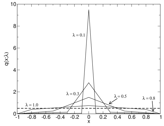
Figure 1: Graphs of $q(x;\lambda)$ for several values of $\lambda$. The function approximates the delta function as $\lambda\rightarrow 0$, and the uniform distribution as $\lambda\rightarrow 1$. The plot for $\lambda=1$ is shown as a dashed line.

$q$ is symmetric and piecewise linear in $x$. $\lambda\in(0,1)$ is the adjustable width. From the normalization condition, we get the height of the distribution $\alpha=\frac{1}{\lambda}-\frac{1}{2}$. Fig. 1 shows plots of $q(x;\lambda)$ for some values of $\lambda$ . For the trial move, first pick at random a lattice site $i$, then draw a random variable $x$ from the distribution $q(x;\lambda)$, and then update the spin as

$$\theta_{i}^{\prime}=\theta_{i}+\pi x.$$ (14)

The width of the distribution $\lambda$ is specified by the step size $\delta(E)$. When step size is small, i.e. $\delta(E)\ll 1$, $q(x;\delta(E))$ is a delta function sharply centered at $x=0$, and the new configuration $\theta^{\prime}_{i}$ is close to the current one $\theta_{i}$. When the step size is large, i.e. $\delta(E)\approx 1$, $q(x;\delta(E))$ approximates the uniform distribution, and the new configuration is uncorrelated with the current one. $q(x;\lambda)$ satisfies our requirements for an adjustable distribution and is simple enough to allow us to sample $x$ efficiently footnote03 .

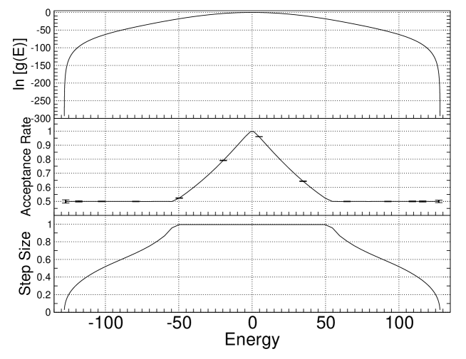
Figure 2: The relationships between the density of states (top panel), acceptance rate (middle panel), and step sizes (bottom panel) for the $XY$ model ($L$=8) obtained using AdaWL. Step sizes are adjusted to keep an optimum acceptance ratio of $0.5$. Between energies $-50$ to $50$, step sizes saturate to a maximum value of $\lambda=1$. Some representative error bars are shown for the acceptance rate.

We also bin the energy levels non-uniformly. The top panel of Fig. 2 shows the DOS of the $XY$ model for $L=8$. The DOS is symmetric, is relatively flat around $E=0$, and drops abruptly near the minimum and maximum energies $E_{min}$ and $E_{max}$. Hence, in both our WLS and AdaWL simulations, we assign smaller energy bins near $E_{min}$ and $E_{max}$ in order to represent the DOS near the edges more accurately. This is accomplished by using the following formula to assign the negative energies,

$$E_{i+1}=E_{i}+w_{c}\exp(-\gamma|E_{i}|^{c})\hskip 4.26773pt\mathrm{for}\hskip 4.26773ptE_{i+1}<0.$$ (15)

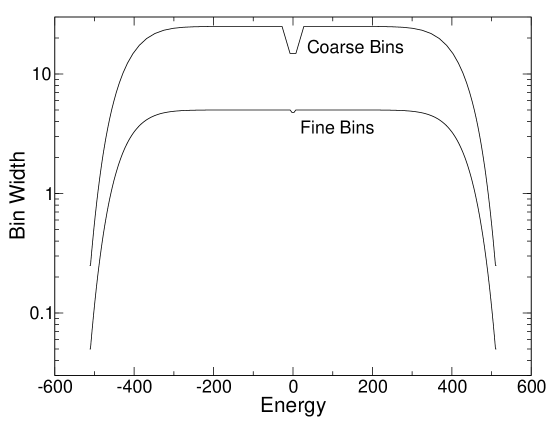
Figure 3: Graphs of bin width versus energy used for the $XY$ model for $L=16$. The widths are larger near $E=0$ and smaller near $E=E_{min}=E_{max}$. The lower graph (fine bins) is the binning scheme given in Table 1 and used throughout this paper (for $L=16$). The upper graph (coarse bins) is discussed in the text.

The initial energy level is given by $E_{0}=E_{min}$. The gaussian-like exponential term in Eq. (15) is to make neighboring energies close near $E_{min}$ where the DOS drops abruptly, but far apart near $E=0$. The constants $c$, $w_{c}$, and width of the initial bin $w(E_{0})=E_{1}-E_{0}$ are set manually. $c$ is a positive even integer that controls the rate of increase of the exponential term. $w_{c}$ is the width at $E=0$. $\gamma$ is determined once $c$, $w_{c}$, and $w(E_{0})$ have been specified. The binning parameters we used are listed in Table 1. The negative energies are reflected about $E=0$ to obtain the positive energies. The bottom graph in Fig. 3 shows the bin widths we used for $L=16$ in the simulations of this paper.

IV Numerical Calculations

The procedure for our numerical simulation of WLS and AdaWL is as follows. The binning of energies are set using Eq. (15). At the start of the simulation, $\ln f_{0}=1$. The modification factor is reduced in stages as $\ln f_{k+1}=\frac{1}{2}\ln f_{k}$, where in the final stage $\bar{k}$ we have $\ln f_{\bar{k}}$. For each stage, we perform simulation until the error of the DOS saturates for that stage before reducing the modification factor. The error of the DOS will be discussed in detail in Section IV.3. For each system size $L$, we computed a total of $N_{traj}$ independent trajectories where each trajectory is started using a different random seed. The details of the simulation parameters are summarized in Table 1.

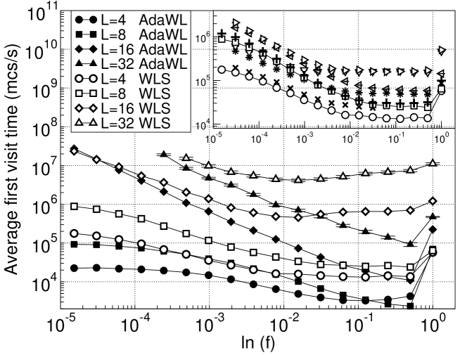
Figure 4: Graphs of the average first visit time versus $\ln{f_{k}}$ for AdaWL and WLS (constant step size 0.05). Errorbar when not shown is smaller than the size of the symbol. Insert: First visit times of WLS for different step sizes. The most efficient step size for WLS is 0.05, with the smallest first visit time. Symbols for insert are as follows. For $L$=4: $*$ for step size=0.01, $\circ$ for 0.05, $\times$ for 0.1, and $\triangledown$ for 0.5. For $L$=8: $\triangleleft$ for step size=0.01, $\square$ for 0.05, $+$ for 0.1, and $\triangleright$ for 0.5.

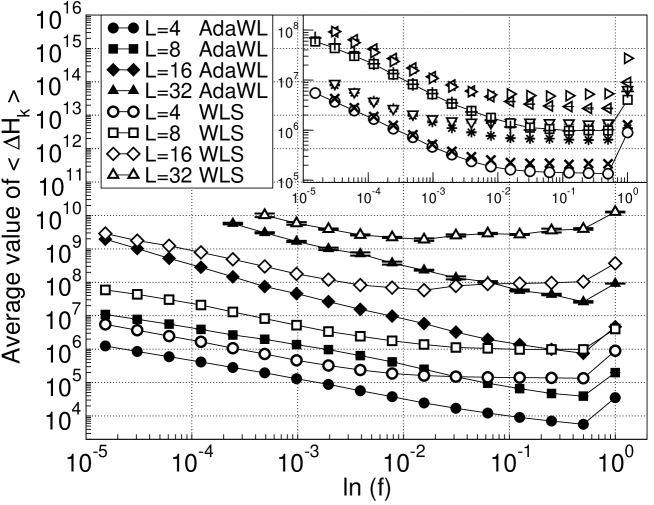
Figure 5: Graphs of average of saturation value of $\langle\Delta H_{k}\rangle$ versus $\ln f_{k}$ for AdaWL and WLS (constant step size=0.05). Insert: For WLS with different step sizes. Symbols have the same meaning as Fig. 4. The most efficient step size for WLS is 0.05, which has the lowest saturation values.

For WLS, our trial moves are also given by Eq. (13) with $\lambda$ being a constant $\delta_{0}$. We have experimented with several constant step sizes and found $\delta_{0}=0.05$ to perform the best. The numerical results supporting this claim are presented in subsections IV.2 and IV.3 and the insets of Figs. 4 and 5. In the rest of the paper, unless otherwise stated, we shall be comparing AdaWL with WLS of step size 0.05.

For AdaWL, the step sizes are $\delta(E_{i})=1$ for all $E_{i}$ at the start of the simulation. During simulation, we also accumulate $A(E)$ and $R(E)$. Once every $\approx 10^{5}$ single site updates per spin, we use Eqs. (6) and (7) to update the step sizes. $A(E)$ and $R(E)$ are then reset to zero, and their accumulation restarted for the next iteration of step size update. During simulations, the curves for $P(E)$ and $\delta(E)$ converged very quickly (i.e. after a few iterations of Eqs. (6) and (7)). Fig. 2 shows the DOS, $P(E)$, and $\delta(E)$ of our AdaWL simulation for $L=8$. As can be seen, Eq. (6) adjusts the step sizes such that the acceptance rate is $0.5$. In the high DOS energy range between -50 and 50, the acceptance rate did not reach $0.5$ because the step size has already saturated to the maximum of 1 and the acceptance rate cannot be further optimized. The DOS is updated quickly with the maximal modification factor in this energy range. Near the edges of the DOS, the step size and modification factors are both small, and the DOS is updated gradually.

In the following, we compare the performance between WLS and AdaWL using three different measures: (1) the specific heat capacity, (2) the first visit time, and (3) the saturation of DOS error.

IV.1 Specific heat capacity

We first demonstrate that AdaWL computes the correct DOS, and that it is more accurate than WLS . To do that, we compute the specific heat capacity. We first divide $N_{traj}$ into four equal portions. For each portion, we compute the mean of the DOS (i.e. we average over the final DOS’s of the $N_{traj}/4$ trajectories). This average DOS is used to compute the specific heat capacity per spin $c_{v}$ at temperature $T$ using

$$c_{v}=\frac{\langle E^{2}\rangle-\langle E\rangle^{2}}{T^{2}L^{2}},$$ (16)

where the thermal average of $f(E)$ is given by

$$\langle f(E)\rangle=\int_{E_{min}}^{E_{max}}f(E)g(E)e^{-E/T}\,\,\mathrm{d}E.$$ (17)

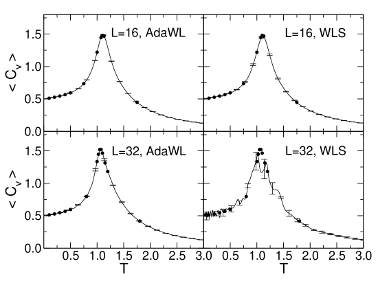
Figure 6: Graphs of average specific heat capacities $\langle c_{v}\rangle$ calculated using AdaWL (left) and WLS (right) for $L=16$ (top) and $32$ (bottom). Solid circles indicate values obtained using Metropolis algorithm.

The $c_{v}$ is then further averaged over the four portions. We denote this specific heat averaged over the four portions as $\langle c_{v}\rangle$. Fig. 6 shows the results of $\langle c_{v}\rangle$ for $L=16$ and $32$. The left (right) panels are for AdaWL (WLS). $\langle c_{v}\rangle$ is given by the solid curve. The standard error at some temperatures is also indicated using error bars. The size of the error bars show that the precision of the specific heat calculated by AdaWL is better than that of WLS. For $L=32$, it is apparent that WLS produces a grossly incorrect curve for $\langle c_{v}\rangle$. To check the accuracy of the AdaWL results, we performed Metropolis simulations to generate accurate specific heat capacity values at selected temperatures, and these are also plotted for comparison in Fig. 6 using solid circles. The $\langle c_{v}\rangle$ curves from AdaWL agree very well with the results of Metropolis calculations. The actual $\langle c_{v}\rangle$ values from all three methods are also listed in Tables 2 ($L=16$) and 3 ($L=32$). We see that AdaWL is consistently closer to the benchmarked Metropolis numbers compared to WLS.

The simulation parameters of our Metropolis calculations are listed in Table 1.

IV.2 Ergodicity of the random walker: first visit time

One way to measure the performance of a random sampler is its ergodicity. The more ergodic the sampler, the more efficient it is in exploring representative parts of phase space. For the Wang-Landau algorithm, some authors have used the so-called tunneling time as a measure of ergodicity Poulain06 . This is the time it takes for the random walker to go from one energy minimum configuration to another. The shorter the tunneling time, the more ergordic is the random walker.

Here, we adopt a related measure of ergodicity which is much easier to compute—the first visit time. At the start of each $\ln f$ stage of the WLS or AdaWL simulation when the modification factor has just been decreased, the histogram is zero for all energy bins. The first visit time is defined as the time it takes for all the bins of the histogram to be visited at least once by the random walker. For each trajectory, we compute one first visit time for each $\ln f$ stage of the simulation. We then average over $N_{traj}$ trajectories. Fig. 4 shows the results. The average first visit times is plotted against $\ln{f_{k}}$ for AdaWL and WLS for various system size. Generally, AdaWL (filled symbols) visits all energy levels much faster than WLS (empty symbols) at all stages and for all system sizes, implying better ergodicity. The insert is a similar plot comparing the results for WLS with different constant step sizes; a constant step size of $0.05$ performs the best for WLS. The first visit time at small $\ln f$ for $L=16$ is similar for AdaWL and WLS. We attribute this to binning effects which will be discussed in Section IV.4.

In their study of the $XY$ model, Sinha and RoySinha09 reported that the random walker of WLS frequently does not visit energy bins near $E_{min}$ and $E_{max}$. Here, we mention that our bins near the edges are much smaller and also nearer to $E_{min}$ and $E_{max}$ compared to what Sinha and Roy had used. That AdaWL has no difficulty sampling all energy bins is indicative that it performs better than WLS.

IV.3 Saturation of DOS error

We now consider the error in the DOS. In Wang and Landau’s original formulation, the ‘flatness of histogram’ criterion was used as a measure of convergence of the WLS. Each stage of the sampling was performed until the accumulated histogram becomes sufficiently flat before the modification factor is reduced. However, it is now known that this is not a good measure of convergence because the height of the histogram increases linearly with time and will ultimately reach flatness regardless of whether the simulation for that stage has converged or not. Detailed studies by various authors on the DOS error of WLS have revealed that the error is related to the modification factor instead of histogram flatness Zhou05 . Also, the use of arbitrary histogram flatness as a criterion has been shown to lead to non-convergence of WLS by Yan03 ; Morozov09 . The correct convergence of WLS has also been proposed by Morozov and Lin Morozov07 .

In a separate investigation, Lee et. al. Lee06 formulated a more precise measure of the convergence of WLS which is shown to agree with the $\sqrt{\ln f}$ analysis by Zhou and Bhatt. Details will be presented in Appendix B. Here we shall present the main idea. Denote the histogram for the $k$th stage of the simulation as $H_{k}(E)$. We define a new histogram $\tilde{H}_{k}(E)$ obtained by subtracting away the minimum value of $H_{k}(E)$, i.e.

$$\tilde{H}_{k}(E)=H_{k}(E)-\min_{E}\{H_{k}(E)\}.$$ (18)

Hence, $\tilde{H}_{k}(E)$ is not plagued by the problem of linear growth. The area under $\tilde{H}_{k}(E)$

$$\Delta H_{k}=\sum_{E}w(E)\tilde{H}_{k}(E),$$ (19)

is conjectured by Lee, Okabe, and Landau to be a measure of the error in the DOS Lee06 . (The $w(E)$ in Eq. (19) is to account for the non-uniform energy bin widths.) During each stage of the simulation, $\Delta H_{k}$ first increases and then saturates to around some mean value. This means that further sampling will not help to reduce the error in the DOS, and therefore the modification factor should be reduced. Note that an increasing $\Delta H_{k}$ does not mean increasing error in the DOS, because the actual error has to take into account the smallness of the modification factor (c.f. Eq. (23)). The key observation is the saturation of $\Delta H_{k}$ during each stage of the simulation. Lee et. al. Lee06 applied $\Delta H_{k}$ to study the DOS error of WLS in the two-dimension Ising model where the exact numerical solution for the DOS is available, and found that it is a good measure of the DOS convergence. It has also been applied by Sinha and Roy to study WLS of the $XY$ model Sinha09 .

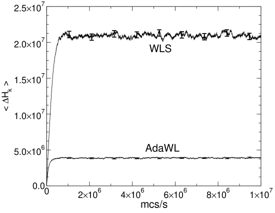
Figure 7: Saturation curves of $\langle\Delta H_{k}\rangle$ for AdaWL and WLS at $\ln f=(1/2)^{14}$ for $L$=8 .

Fig. 7 shows an example of the saturation of $\Delta H_{k}$ for the $XY$ model. It compares the saturation curves for AdaWL and WLS at the modification factor $\ln f=(1/2)^{14}$ for $L=8$. Each curve $\langle\Delta H_{k}\rangle$ is obtained by averaging over $N_{traj}$ trajectories. It can be seen that both WLS and AdaWL curves saturate to some constant value after a certain number of Monte Carlo steps. However, the saturation value of AdaWL is much smaller than WLS, implying a smaller error for AdaWL.

For the simulations in this paper, we ran the simulation at each stage long enough to obtain accurate saturation values of $\langle\Delta H_{k}\rangle$. Although in practice $\ln f_{k}$ should be decreased as soon as saturation is reached, as our purpose here is to compare the performance of AdaWL and WLS, we ran each stage much longer than is necessary to obtain reliable measurements of $\Delta H_{k}$.

We now describe how we compare the DOS saturation error of AdaWL and WLS. The $N_{traj}$ trajectories are first divided into four equal portions. For each portion, at each stage $k$, we compute $\langle\Delta H_{k}\rangle$ curves similar to that of Fig. 7 by averaging $\Delta H_{k}$ over $N_{traj}/4$ trajectories. Using this averaged curve $\langle\Delta H_{k}\rangle$, we estimate its saturation value by averaging over the time steps in the flat part (say last 10 percent) of the curve. This gives us the saturation value of $\langle\Delta H_{k}\rangle$ of that stage for that one portion. We then average the saturation value over all four portions. The results are shown in Fig. 5. The average saturation value of $\langle\Delta H_{k}\rangle$ is plotted against $\ln f_{k}$ for AdaWL and WLS for various system size. AdaWL (filled symbols) has significantly smaller saturation values than WLS (empty symbols), implying a smaller error in the DOS. The insert is a similar plot comparing the results for WLS with different constant step sizes; a constant step size of 0.05 gives the smallest saturation value for WLS.

IV.4 Non-uniform binning of energy levels

Lastly, we briefly comment on the use of non-uniform energy bin widths. When using non-uniform bin widths in Wang-Landau simulations, there is the freedom to choose large energy spacings at certain energies. However, to compute thermodynamic quantities such as the specific heat capacity accurately, the spacings between energy levels has to be small enough to enable a good representation of the distribution $g(E)e^{-E/T}$ at the temperatures of interests. Hence, it is recommended that one first check by making a rough plot of $g(E)e^{-E/T}$ to ensure that it is represented with a sufficient number of energy levels at the temperatures concerned. This is especially important for large system size because the appearances of singularities or cusps usually require finer energy spacings to resolve. Of course, the spacings also cannot be too small otherwise each bin will not accumulate enough visits by the random walker.

In this paper, we have used Eq. (15) to set our energy levels. It might be tempting to choose $c$ and $w_{c}$ to be quite large, thereby greatly reducing the number of energy levels used, especially near $E=0$. However, we found that this will lead to an insufficient number of energy levels representing $g(E)e^{-E/T}$ at lower temperatures. Our choice of binning parameters in Table 1 ensures a good representation of $g(E)e^{-E/T}$.

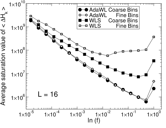
Figure 8: Plots showing the effects of bin widths. AdaWL is robust against changes in bin widths. WLS becomes less efficient for the fine bins, this is due to WLS’s inefficiency in sampling the fine bins very near the ground state.

We have also studied the effects of different bin widths on AdaWL and WLS, and found that there might be rare instances where WLS appears to give similar performances as AdaWL. But these rare cases are usually due to effects of bin widths. If one uses coarse bins, WLS can reach all bins easily, whereas if a finer set of bin widths near the ground state is used, WLS will have difficulty visiting those small bins. AdaWL, however, will not show such dependence because its step size is designed to be adaptively adjusted according to the energies. In Fig. 4, WLS shows signs of smaller first visit time than AdaWL towards the smaller $\ln f$ for $L=16$. We have found that using even finer bin widths will increase the first visit time for WLS , but not for AdaWL. However, since we have already obtained a more accurate specific heat capacity for AdaWL at that bin width, we did not pursue to further accentuate the performance between the two methods. As another example, Fig. 8 compares the saturated DOS error of AdaWL and WLS for the coarse and fine bin widths shown in Fig. 3. AdaWL gives the same results for both sets of bin widths, whereas the error for WLS increases for the fine bin widths.

V Discussion and conclusion

To summarize, we proposed an adaptive variant of the Wang-Landau sampling, which is effective for sampling DOS that ranges many orders of magnitude. The main contributing factors to this increase in efficiency are adaptive step sizes and adaptive modification factors. Adaptive step sizes sample the configuration space well, while adaptive modification factors accumulate the DOS effectively and accurately. We have tested the effectiveness of AdaWL for system sizes up to $L$=32. For larger sizes, we may break into several energy regions Wang01a , where the method to avoid “boundary effect” should be taken into account Schulz03 . In such a case, the present adaptive method is still effective for treating DOS that has many orders of magnitude. For future work, AdaWL should be tested on different continuous systems, especially frustrated ones.

In Fig. 2, we see that AdaWL is not yet fully optimized because the acceptance rate in the middle energy range has not been adjusted to 0.5 due to the saturation of $\delta(E)$ to the maximum value of 1. At larger lattice sizes, where the energy range is larger, one might consider going beyond single site updates (e.g. global moves) to enable even larger step sizes to be used. This might make the sampling of AdaWL even more efficient.

Recently, there have been many works on improving WLS both for discrete Schulz03 ; Zhou05 ; Troster05 ; Belardinelli07b ; Zhou08 ; Belardinelli08 ; Cunha-Netto08 ; Cunha-Netto11 ; Brown11 and continuous Shell02 ; Poulain06 ; Swetnam10 ; Jayasri05 ; Zhou06 systems. To obtain better convergence, the $1/t$ algorithm Belardinelli07b was proposed. Moreover, tomographic entropic sampling scheme dickman was proposed as an algorithm to calculate DOS. The convergence of WLS was discussed with paying attention to the difference of density of states by Komura and Okabe Komura12 . It will be interesting to combine the present work with the recent progress. Finally, we make a note that our idea of using an adaptive modification factor could potentially be used for simulating discrete systems as well as continuous systems. This will also be part of our future work.

VI Acknowledgements

This work was supported (in part) by the Biomedical Research Council of A*STAR (Agency for Science, Technology and Research), Singapore.

Appendix A Summary of AdaWL Algorithm

Our AdaWL algorithm is as follows.

1. Initialize the bin sizes $w(E_{i})$ according to Eq. (15). Initialize the system configuration $\sigma$, the DOS $\ln g(E_{i})=0$, the histogram $H(E_{i})=0$, modification factor $\ln f_{0}$, and step sizes $\delta(E_{i})$=constant.

2. Sample a new configuration $\sigma^{\prime}$ from $T(\sigma^{\prime}|\sigma;\delta(E))$ and accept the move as given by Eq. (8).

3. Update the DOS and histogram according to Eq. (10). Update the acceptance and rejection counts $A(E_{i})$ and $R(E_{i})$.

4. Repeat steps 2 and 3 for some predefined number of Monte Carlo steps and update the step size according to Eq. (6). Set $A(E_{i})=R(E_{i})=0$.

5. Reduce $\ln f_{k}$ (e.g., $\ln f_{k}\leftarrow\ln f_{k}/2$, after the DOS error saturates) and set $H(E_{i})=0$; else, repeat Steps 2 to 4.

6. Repeat steps 2 to 5 until the modification factor $\ln f_{k}$ is smaller than some tolerance threshold.

Appendix B Detailed presentation of the measure $\Delta H_{k}$

The contents of this appendix was first given in Lee et. al. Lee06 . The reader is referred there for a more complete presentation. Here, for completeness, we outline the main idea presented there, and also update the analysis to take into account the use of non-uniform energy bin widths.

The DOS $\ln g_{n}(E)$ accumulated after the $n$th stage can be written as

$$\ln g_{n}(E)=\sum_{k=1}^{n}H_{k}(E)\ln(f_{k})$$ (20)

where $H_{k}(E)$ is the accumulated histogram and $\ln f_{k}$ is the modification factor for the $k$th stage of simulation. Eq. (20) holds for both WLS and AdaWL. Calculation of thermodynamics quantities are not affected if we subtract a constant from $H_{k}(E)$, hence we subtract the minimum of $H_{k}(E)$,

$$\tilde{H}_{k}(E)=H_{k}(E)-\min_{E}\{H_{k}(E)\}$$ (21)

and define a new but equally valid density of states,

$$\ln\tilde{g}_{n}(E)=\sum_{k=1}^{n}\tilde{H}_{k}(E)\ln(f_{k}).$$ (22)

To introduce our histogram measure, we observe that it is reasonable to estimate the error between the computed density of states $\tilde{g}_{n}(E)$ and the true one $\tilde{g}_{\infty}(E)$ as

$$\sum_{E}w(E)[\ln\tilde{g}_{\infty}(E)-\ln\tilde{g}_{n}(E)]=\sum_{E}\sum_{k=n+1}^{\infty}w(E)\tilde{H}_{k}(E)\ln(f_{k})$$ (23)

An intuitive view of Eq. (23) is that if an infinite number of stages were performed (i.e. $n\rightarrow\infty$), then the exact DOS will be obtained. This statement was made formal by the conjecture of Lee, Okabe and Landau Lee06 . If just $n$ stages were done instead, the error of $\tilde{g}_{n}(E)$ will be the sum of all the rest of the stages that were not carried out explicitly. We denote the fluctuation of $\tilde{H}_{k}(E)$ as

$$\Delta H_{k}=\sum_{E}w(E)\tilde{H}_{k}(E).$$ (24)

Note that the summation over $E$ in Eq. (24) includes the binwidth $w(E)$. This is a slight modification from the original formulation. Swapping the order of summation, the RHS of Eq. (23) becomes

$$\sum_{k=n+1}^{\infty}\Delta H_{k}\ln(f_{k})$$ (25)

Hence, the error depends only on $\Delta H_{k}$ and the sequence of modification factors $\ln f_{k}$. If $\ln f_{k}$ are predetermined, then $\Delta H_{k}$ becomes the only determining factor of the error. Hence, when we see that it saturates (for a certain $k$), it is an indication that enough statistics has been accumulated for this $\ln f_{k}$ value and simulation for the next value $\ln f_{k+1}$ should begin. Finally, it is important to note that smaller $\Delta H_{k}$ values indicates that the accumulated histogram is flatter.

System	AdaWL and WLS								Metropolis
	Energy binning			AdaWL only		WLS only ($\delta_{0}=0.05$)
$L$	$w(E_{0})$	$w_{c}$	$c$	$\ln f_{\bar{k}}$	$N^{\bar{k}}$ ($\times 10^{7}$)	$\ln f_{\bar{k}}$	$N^{\bar{k}}$($\times 10^{7}$)	$N_{traj}$	$N_{MC}$($\times 10^{7}$)	$N_{traj}$
4	0.01	0.5	10	$2^{-17}$	6	$2^{-17}$	6	1000	5	10
8	0.05	5.0	10	$2^{-17}$	6	$2^{-17}$	6	1000	1	10
16	0.05	5.0	10	$2^{-17}$	75	$2^{-17}$	60	200	1	10
32	0.10	5.0	10	$2^{-13}$	15	$2^{-12}$	10	100	1	10

Table 1: Summary of parameters used in AdaWL, WLS, and Metropolis simulations. $\delta_{0}$: Constant step size used for WLS ($\lambda$ in Eq. (13)). $\ln f_{\bar{k}}$: Smallest (i.e. final) modification factor used in simulation. $N^{\bar{k}}$: No. of single site updates per spin used for $\ln f_{\bar{k}}$ (the final stage). $N_{MC}$: No. of single site updates per spin used for Metropolis simulation. Parameter values for Eq. (6): $P_{\mathrm{opt}}=0.5$, $a=0.82988$, and $b=0.014625$ footnote01 .

$L=16$
Metropolis			Deviation (units of $\sigma$)
$T$	$\langle c_{v}\rangle$	$\sigma(\times 10^{-4})$	$\langle c_{v}\rangle$ AdaWL	$\langle c_{v}\rangle$ WLS
0.1	0.5112	8	0.3	5
0.2	0.5266	8	0.3	4
0.3	0.5446	6	-1	0.2
0.4	0.5664	5	0.8	5
0.5	0.5948	7	0.03	-5
0.75	0.7358	7	-1	-0.7
1.0	1.2200	20	0.05	3
1.075	1.4467	20	2	-8
1.1	1.4796	30	1	-6
1.13	1.4690	10	3	-11
1.75	0.4483	4	0.5	-8

Table 2: Values of average specific heat capacity, $\langle c_{v}\rangle$, computed using Metropolis, AdaWL, and WLS. The $\langle c_{v}\rangle$ values for Metropolis are computed by averaging over $N_{traj}$ trajectories (c.f. Table 1, under Metropolis). Values of $\langle c_{v}\rangle$ for AdaWL and WLS are listed in terms of their deviation from the $\langle c_{v}\rangle$ of Metropolis (measured in units of $\sigma$, the standard deviation of Metropolis calculations).

$L=32$
Metropolis			Deviation (units of $\sigma$)
$T$	$\langle c_{v}\rangle$	$\sigma(\times 10^{-4})$	$\langle c_{v}\rangle$ AdaWL	$\langle c_{v}\rangle$ WLS
0.1	0.5132	9	10	-20
0.2	0.5283	6	10	-30
0.3	0.5459	5	-4	-100
0.4	0.5683	7	5	10
0.5	0.5966	7	-8	20
0.8	0.7966	5	-10	20
1.0	1.336	30	-2	20
1.025	1.448	30	-7	-10
1.05	1.519	30	-8	-90
1.075	1.521	20	-1	-200
1.1	1.465	30	4	-100
1.15	1.314	10	6	-70
1.2	1.182	20	3	30
1.8	0.4174	2	2	-30

Table 3: Similar to Table 2, but for $L=32$.

References

- (1) F. Wang and D.P. Landau, Phys. Rev. Lett. 86, 2050 (2001); F. Wang and D.P. Landau, Phys. Rev. E 64, 056101 (2001).
- (2) P. Poulain, F. Calvo, R. Antoine, M. Broyer, and Ph. Dugourd, Phys. Rev. E 73, 056704 (2006).
- (3) A.D. Swetnam and M.P. Allen, J. Comput. Chem. 32, 816 (2010); D.T. Seaton, T. Wüst, and D.P. Landau, Phys. Rev. E 81, 011802 (2010); S.Æ. Jónsson, S. Mohanty, and A. Irbäck, J. Chem. Phys. 135, 125102 (2011).
- (4) D. Jayasri, V.S.S. Sastry, and K.P.N. Murthy, Phys. Rev. E 72, 036702 (2005).
- (5) C. Zhou, T. C. Schulthess, S. Torbrugge, D. P. Landau, Phys. Rev. Lett. 96, 120201-1 (2006).
- (6) J. Xu and H-R. Ma, Phys. Rev. E 75, 041115 (2007).
- (7) S. Sinha and S.K. Roy, Phys. Lett. A 373, 308 (2009).
- (8) P.E. Theodorakis and N.G. Fytas, Eur. Phys. J. B 81, 245 (2011).
- (9) C. Zhou and R.N. Bhatt, Phys. Rev. E 72, 025701(R) (2005).
- (10) D. Bouzida, S. Kumar, and R.H. Swendsen, Phys. Rev. A 45, 8894 (1992).
- (11) R. H. Swendsen and J. S. Wang, Phys. Rev. Lett. 58, 86 (1987).
- (12) U. Wolff, Phys. Rev. Lett. 62, 361 (1989).
- (13) J. Liu and E. Luijten, Phys. Rev. Lett. 92, 035504 (2004).
- (14) H. K. Lee and R. H. Swendsen, Phys. Rev. B 64, 214102 (2001).
- (15) H.K. Lee, Y. Okabe, and D.P. Landau, Comput. Phys. Commun. 175, 36 (2006).
- (16) B.J. Schulz, K. Binder, M. Müller, and D.P. Landau, Phys. Rev. E 67, 067102 (2003).
- (17) A. Tröster and C. Dellago, Phys. Rev. E 71, 066705 (2005).
- (18) R.E. Belardinelli and V.D. Pereyra, Phys. Rev. E 75, 046701 (2007).
- (19) R.E. Belardinelli, S. Manzi, and V.D. Pereyra, Phys. Rev. E 78, 067701 (2008).
- (20) C. Zhou and J. Su, Phys. Rev. E 78, 046705 (2008).
- (21) A.G. Cunha-Netto, A.A. Caparica, S-H. Tsai, R. Dickman, and D.P. Landau, Phys. Rev. E 78, 055701(R) (2008).
- (22) A.G. Cunha-Netto and R. Dickman, Comput. Phys. Commun. 182, 719 (2011).
- (23) G. Brown, Kh. Odbadrakh, D.M. Nicholson, and M. Eisenbach, Phys. Rev. E 84, 065702(R) (2011); A.A. Caparica and A.G. Cunha-Netto, Phys. Rev. E 85, 046702 (2012).
- (24) M.S. Shell, P.G. Debenedetti, and A.Z. Panagiotopoulos, Phys. Rev. E 66, 056703 (2002).
- (25) R. Dickman and A. G. Cunha-Netto, Phys. Rev. E 84, 026701 (2011).
- (26) Y. Komura and Y. Okabe, Phys. Rev. E 85, 010102(R) (2012).
- (27) A. N. Morozov and S. H. Lin, Phys. Rev. E 76, 026701 (2007).
- (28) Q. Yan and J. J. de Pablo, Phys. Rev. Lett. 90, 035701 (2003).
- (29) A. N. Morozov and S. H. Lin, J. Chem. Phys. 130, 074903 (2009).
- (30) It is easy to see that the step-size increases (decreases) at each iteration when () until it reaches a fixed point at .
- (31) In their original paper, Bouzida et. al. recommended for one, for two, and for three dimensional trial moves.
- (32) For derivations of the values of and , please refer to Bouzida et. al.Bouzida92 .
- (33) In our calculations for the model below, we used non-uniform binnings for both WLS and AdaWL. Hence, the division by bin width applies to WLS as well.
- (34) We choose Eq. (13) for the trial move transition probability because its cumulative and inverse cumulative distributions can easily be derived analytically, facilitating the numerical calculation of the random variable .