A parallel directional fast multipole method

Abstract

This paper introduces a parallel directional fast multipole method (FMM) for solving $N$-body problems with highly oscillatory kernels, with a focus on the Helmholtz kernel in three dimensions. This class of oscillatory kernels requires a more restrictive low-rank criterion than that of the low-frequency regime, and thus effective parallelizations must adapt to the modified data dependencies. We propose a simple partition at a fixed level of the octree and show that, if the partitions are properly balanced between $p$ processes, the overall runtime is essentially $\mathcal{O}(N\log N/p+p)$. By the structure of the low-rank criterion, we are able to avoid communication at the top of the octree. We demonstrate the effectiveness of our parallelization on several challenging models.

1 Introduction

This paper is concerned with a parallel algorithm for the rapid solution of a class of $N$-body problems. Let $\{f_{i},1\leq i\leq N\}$ be a set of $N$ densities located at points $\{p_{i},1\leq i\leq N\}$ in $\mathbb{R}^{3}$, with $|p_{i}|\leq K/2$, where $|\cdot|$ is the Euclidean norm and $K$ is a fixed constant. Our goal is to compute the potentials $\{u_{i},1\leq i\leq N\}$ defined by

(1) $$u_{i}=\displaystyle\sum\limits_{j=1}^{N}G(p_{i},p_{j})\cdot f_{j},$$

where $G(x,y)=e^{2\pi\iota|x-y|}/|x-y|$ is the Green’s function of the Helmholtz equation. We have scaled the problem such that the wave length equals one and thus high frequencies correspond to problems with large computational domains, i.e., large $K$.

The computation in Equation 1 arises in electromagnetic and acoustic scattering, where the usual partial differential equations are transformed into boundary integral equations (BIEs) [16, 24, 34, 36]. The discretized BIEs often result in large, dense linear systems with $N=O(K^{2})$ unknowns, for which iterative methods are used. Equation 1 represents the matrix-vector multiplication at the core of the iterative methods.

1.1 Previous work

Direct computation of Equation 1 requires $\mathcal{O}(N^{2})$ operations, which can be prohibitively expensive for large values of $N$. A number of methods reduce the computational complexity without compromising accuracy. The approaches include FFT-based methods [2, 3, 6], local Fourier bases [4, 8], and the high frequency fast multipole method (HF-FMM) [9, 13, 27]. We focus on a multilevel algorithm developed by Engquist and Ying which exploits the numerically low-rank interaction satisfying a directional parabolic separation condition [18, 19, 20, 33].

There has been much work on parallelizing the FMM for non-oscillatory kernels [17, 23, 26, 39]. In particular, the kernel-independent fast multipole method (KI-FMM) [37] is a central tool for our algorithm in the “low-frequency regime”, which we will discuss in subsection 2.3. Many efforts have extended KI-FMM to modern, heterogeneous architectures [11, 12, 26, 38, 40], and several authors have paralellized [21, 22, 31, 35] the Multilevel Fast Multipole Algorithm [15, 29, 30], which is a variant of the HF-FMM.

1.2 Contributions

This paper provides the first parallel algorithm for computing Equation 1 based on the directional approach. Since the top of the octree imposes a well-known bottleneck in parallel FMM algorithms [38], a central advantage of the directional approach is that the interaction lists of boxes in the octree with width greater than or equal to $2\sqrt{K}$ are empty. This alleviates the bottleneck, as no translations are needed at those levels of the octree.

Our parallel algorithm is based on a partition of the boxes at a fixed level in the octree amongst the processes (see subsection 3.1). Due to the simple structure of the sequential algorithm, we can leverage the partition into a flexible parallel algorithm. The parallel algorithm is described in § 3, and the results of several numerical experiments are in § 4. As will be seen, the algorithm exhibits good strong scaling up to 1024 cores for several challenging models.

2 Preliminaries

In this section, we review the directional low-rank property of the Helmholtz kernel and the sequential directional algorithm for computing Equation 1 [18]. Proposition 1 in subsection 2.2 shows why the algorithm can avoid computation at the top levels of the octree. We will use this to develop the parallel algorithm in § 3.

2.1 Directional low-rank property

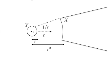
Fig. 1: Sets $Y$ and $X$ that satisfy the directional parabolic separation condition.

Let $Y$ be a ball of radius $r\geq\sqrt{3}$ centered at a point $c$ and define the wedge $X=\{x:\theta(x,\ell)\leq 1/r,|x-c|\geq r^{2}\}$, where $\ell$ is a unit vector and $\theta(x,\ell)$ is the angle between the vectors $x$ and $\ell$. $Y$ and $X$ are said to satisfy the directional parabolic separation condition, which is illustrated in Fig. 1.

Suppose we have a set of charges $\{f_{i}\}$ located at points $\{y_{i}\}\subseteq Y$. Given a threhold $\epsilon$, there exist two sets of points $\{b_{q}\}_{1\leq q\leq r_{\epsilon}}$ and $\{a_{p}\}_{1\leq p\leq r_{\epsilon}}$ and a set of constants $\{d_{pq}\}_{1\leq p,q\leq r_{\epsilon}}$ such that, for $x\in X$,

(2) $$\left|\displaystyle\sum\limits_{i}G(x,y_{i})f_{i}-\displaystyle\sum\limits_{q}G(x,b_{q})\left(\displaystyle\sum\limits_{p}d_{qp}\displaystyle\sum\limits_{i}G(a_{p},y_{i})f_{i}\right)\right|=\mathcal{O}(\epsilon)$$

where $r_{\epsilon}$ is a constant that depends only on $\epsilon$. A random sampling method based on pivoted QR factorization [20] can be used to determine this approximation. We can, of course, reverse the roles of the ball and the wedge. In Equation 2, the quantities $\{\sum_{p}{d_{qp}\sum_{i}{G(a_{p},y_{i})f_{i}}}\}$, $\{b_{q}\}$, $\{\sum_{i}{G(b_{q},x_{i})f_{i}}\}$, and $\{a_{p}\}$ are called the directional outgoing equivalent charges, equivalent points, check potentials, and check points of $Y$ in direction $\ell$. When the roles of $X$ and $Y$ are reversed, $\{\sum_{q}{d_{qp}\sum_{i}{G(b_{q},x_{i})f_{i}}}\}$, $\{a_{p}\}$, $\{\sum_{i}{G(b_{q},x_{i})f_{i}}\}$, $\{b_{q}\}$ are called the directional incoming equivalent charges, equivalent points, check potentials, and check points of $Y$ in direction $\ell$. The constants $d_{pq}$ form a matrix $D=(d_{p,q})$ that we call a translation matrix.

2.2 Definitions

Without loss of generality, we assume that the domain width is $K=2^{2L}$ for a positive integer $L$ (recall that $|p_{i}|\leq K/2$ in Equation 1). The central data structure in the sequential algorithm is an octree. The parallel algorithm, described in § 3, uses the same octree. For the remainder of the paper, let $B$ denote a box in the octree and $w(B)$ the width of $B$. We say that a box $B$ is in the high-frequency regime if $w(B)\geq 1$ and in the low-frequency regime if $w(B)<1$. As discussed in [18], the octree is non-adaptive in the non-empty boxes of the high-frequency regime and adaptive in the low-frequency regime. In other words, a box $B$ is partitioned into children boxes if $B$ is non-empty and in the high-frequency regime or if the number of points in $B$ is greater than a fixed constant and in the low-frequency regime.

For each box $B$ in the high-frequency regime and each direction $\ell$, we use the following notation for the relevant data:

• $\{y_{k}^{B,o,\ell}\}$, $\{f_{k}^{B,o,\ell}\}$, $\{x_{k}^{B,o,\ell}\}$, and $\{u_{k}^{B,o,\ell}\}$ are the outgoing directional equivalent points, equivalent charges, check points, and check potentials, and

• $\{y_{k}^{B,i,\ell}\}$, $\{f_{k}^{B,i,\ell}\}$, $\{x_{k}^{B,i,\ell}\}$, and $\{u_{k}^{B,i,\ell}\}$ are the incoming directional equivalent points, equivalent charges, check points, and check potentials.

In the low-frequency regime, the algorithm uses the kernel-independent FMM [37]. For each box $B$ in the low-frequency regime, we use the following notation for the relevant data:

• $\{y_{k}^{B,o}\}$, $\{f_{k}^{B,o}\}$, $\{x_{k}^{B,o}\}$, and $\{u_{k}^{B,o}\}$ are the outgoing equivalent points, equivalent charges, check points, and check potentials, and

• $\{y_{k}^{B,i}\}$, $\{f_{k}^{B,i}\}$, $\{x_{k}^{B,i}\}$, and $\{u_{k}^{B,i}\}$ are the incoming equivalent points, equivalent charges, check points, and check potentials.

Due to the translational and rotational invariance of the relevant kernels, the (directional) outgoing and incoming equivalent and check points can be efficiently precomputed since they only depend upon the problem size, $K$, and the desired accuracy. We discuss the number of equivalent points and check points in subsection 4.1.

Let $B$ be a box with center $c$ and $w(B)\geq 1$. We define the near field of a box $B$ in the high-frequency regime, $N^{B}$, as the union of boxes $A$ that contain a point in a ball centered at $c$ with radius $\sqrt{3}w/2$. Such boxes are too close to satisfy the directional parabolic condition described in subsection 2.1. The far field of a box $B$, $F^{B}$, is simply the complement of $N^{B}$. The interaction list of $B$, $I^{B}$, is the set of boxes $N^{P}\backslash N^{B}$, where $P$ is the parent box of $B$.

To exploit the low-rank structure of boxes separated by the directional parabolic condition, we need to partition $F^{B}$ into wedges with a spanning angle of $\mathcal{O}(1/w)$. To form the directional wedges, we use the construction described in [18]. The construction has a hierarchical property: for any directional index $\ell$ of a box $B$, there exists a directional index $\ell^{\prime}$ for boxes of width $w(B)/2$ such that the $\ell$-th wedge of $B$ is contained in the $\ell^{\prime}$-th wedge of $B$’s children. Figure 2 illustrates this idea. In order to avoid boxes on the boundary of two wedges, the wedges are overlapped. Boxes that would be on the boundary of two wedges are assigned to the wedge that comes first in an arbitrary lexicographic ordering.

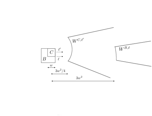
Fig. 2: A two-dimensional slice of the three-dimensional hierarchical wedges. $W^{B,\ell}$ is the wedge for box $B$ for the directional index $\ell$. By the hierarchical construction, we can find an index direction $\ell^{\prime}$ such that for any child box $C$ of $B$, $W^{B,\ell}$ is contained in $W^{C,\ell^{\prime}}$, the $\ell^{\prime}$-th wedge of $C$. Since $C$ has a smaller width ($w$) than $B$ ($2w$), the wedge for $C$ is closer and wider than the wedge for $B$. This is a consequence of the directional parabolic separation condition described in subsection 2.1.

2.3 Sequential algorithm

In the high-frequency regime, the algorithm uses directional M2M, M2L, and L2L translation operators [18], similar to the standard FMM [14]. The high-frequency directional FMM operators are as follows:

• HF-M2M constructs the outgoing directional equivalent charges of $B$ from the outgoing equivalent charges of $B$’s children,

• HF-L2L constructs the incoming directional check potentials of $B$’s children from the incoming directional check potentials of $B$, and

• HF-M2L adds to the incoming directional check potentials of $B$ due to outgoing directional charges from each box $A\in I^{B}$.

The following proposition shows that at the top levels of the octree, the interaction lists are empty:

Proposition 1.

Let $B$ be a box with width $w$. If $w\geq 2\sqrt{K}$, then $N^{B}$ contains all nonempty boxes in the octree.

Proof.

Let $c$ be the center of $B$. Then for any point $p_{i}\in B$, $|p_{i}-c|\leq\sqrt{3}w/2$. For any point $p_{j}$ in a box $A$, $|p_{j}-c|\leq|p_{j}|+|p_{i}|+|p_{i}-c|\leq K+\sqrt{3}w/2$. $N^{B}$ contains all boxes $A$ such that there is an $x\in A$ with $|x-c|\leq 3w^{2}/4$. Thus, $N^{B}$ will contain all non-empty boxes if $3w^{2}/4\geq\sqrt{3}w/2+K$. This is satisfied for $w\geq\sqrt{4K/3+1/3}+\sqrt{1/3}$. Since $K=2^{2L}$, this simplifies to $w\geq 2\sqrt{K}$. ∎

Thus, if $w(B)\geq 2\sqrt{K}$, no HF-M2L translations are performed ($I^{B}=\emptyset$). As a consequence, no HF-M2M or HF-M2L translations are needed for those boxes. This property of the algorithm is crucial for the construction of the parallel algorithm that we present in § 3.

We denote the corresponding low-frequency translation operators as LF-M2M, LF-L2L, and LF-M2L. We also denote the interaction list of a box in the low frequency regime by $I^{B}$, although the definition of $N^{B}$ is different [18]. Algorithm 1 presents the sequential algorithm in terms of the high- and low-frequency translation operators.

Data: points $\{p_{i}\}_{1\leq i\leq N}$, densities $\{f_{i}\}_{1\leq i\leq N}$, and octree $\mathcal{T}$

Result: potentials $\{u_{i}\}_{1\leq i\leq N}$

foreach box $B$ in postorder traversal of $\mathcal{T}$ with $w(B)<1$ do

       foreach child box $C$ of $B$ do

             Transform $\{f_{k}^{C,o}\}$ to $\{f_{k}^{B,o}\}$ via LF-M2M

            

      

foreach box $B$ in postorder traversal of $\mathcal{T}$ with $1\leq w(B)\leq\sqrt{K}$ do

       foreach direction $\ell$ of $B$ do

             Let the $\ell^{\prime}$-th wedge of $B$’s children contain the $\ell$-th wedge of $B$

             foreach child box $C$ of $B$ do

                   Transform $\{f_{k}^{C,o,\ell^{\prime}}\}$ to $\{f_{k}^{B,o,\ell}\}$ via HF-M2M

            

      

foreach box $B$ in preorder traversal of $\mathcal{T}$ with $1\leq w(B)\leq\sqrt{K}$ do

       foreach direction $\ell$ of $B$ do

             foreach box $A\in I^{B}$ in direction $\ell$ do

                   Let $\ell^{\prime}$ be the direction for which $B\in I^{A}$

                   Transform $\{f_{k}^{A,o,\ell^{\prime}}\}$ via HF-M2L and add result to $\{u_{k}^{B,i,\ell}\}$

            foreach child box $C$ of $B$ do

                   Transform $\{u_{k}^{B,i,\ell}\}$ to $\{u_{k}^{C,i,\ell}\}$ via HF-L2L

            

      

foreach box $B$ in preorder traversal of $\mathcal{T}$ with $w(B)<1$ do

       foreach $A\in I^{B}$ do

             Transform $\{f_{k}^{A,o}\}$ via LF-M2L and add the result to $\{u_{k}^{B,i}\}$

      Transform $\{u_{k}^{B,i}\}$ via LF-L2L

       if $B$ is a leaf box then

             foreach $p_{i}\in B$ do

                  Add result to $u_{i}$

            

      else

             foreach child box $C$ of $B$ do

                  Add result to $\{u_{k}^{C,i}\}$

            

      

Algorithm 1 Sequential directional FMM for Equation 1.

3 Parallelization

The overall structure of our proposed parallel algorithm is similar to the sequential algorithm. A partition of the boxes at a fixed level in the octree governs the parallelism, and this partition is described in subsection 3.1. We analyze the communication and computation complexities in subsections 3.4 and 3.5. For the remainder of the paper, we use $p$ to denote the total number of processes.

3.1 Partitioning the octree

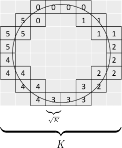
Fig. 3: Two-dimensional slice of the octree at the partition level for a spherical geometry with each box numbered with the process it is assigned to. The width of the boxes at the partition level is $\sqrt{K}$, which ensures that the interaction lists of all boxes above this partition level are empty. We note that the number of boxes with surface points (black border) is much smaller than the total number of boxes.

To parallelize the computation, we partition the octree at a fixed level. Number the levels of the octree such that the $l$-th level consists of a $2^{l}\times 2^{l}\times 2^{l}$ grid of boxes of width $K\cdot 2^{-l}$. By Proposition 1, there are no dependencies between boxes with width strictly greater than $\sqrt{K}$. The partition assigns a process to every box $B$ with $w(B)=\sqrt{K}$, and we denote the partition by $\mathcal{P}$. In other words, for every non-empty box $B$ at level $L$ in the octree (recall that $K=2^{2L}$), $\mathcal{P}(B)\in\{0,1,\ldots,p-1\}$. We refer to level $L$ as the partition level. Process $\mathcal{P}(B)$ is responsible for all computations associated with box $B$ and the descendent boxes of $B$ in the octree, and so we also define $\mathcal{P}(A)\equiv\mathcal{P}(B)$ for any box $A\subset B$. An example partition is illustrated in Figure 3.

3.2 Communication

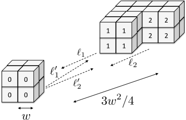
Fig. 4: Interaction in the high-frequency regime that induces communication in the parallel algorithm. In this case, process $0$ needs outgoing directional equivalent densities in direction $\ell_{1}$ from process $1$ and direction $\ell_{2}$ from process $2$. The equivalent densities are translated to incoming directional potentials in the directions $\ell_{1}^{\prime}$ and $\ell_{2}^{\prime}$ via HF-M2L. Similarly, processes $1$ and $2$ needs outgoing directional equivalent densities in direction $\ell_{1}^{\prime}$ and $\ell_{2}^{\prime}$ from process $0$.

We assume that the ownership of point and densities conforms to the partition $\mathcal{P}$, i.e., each process owns exactly the points and densities needed for its computations. In practice, arbitrary point and density distributions can be handled with a simple pre-processing stage. Our later experiments make use of k-means clustering [25] to distribute the points to processes.

The partition $\mathcal{P}$ dictates the communication in our algorithm. Since ${\mathcal{P}(C)=\mathcal{P}(B)}$ for any any child box $C$ of $B$, there is no communication for the L2L or M2M translations in both the-low frequency and high-frequency regimes. These translations are performed in serial on each process. All communication is induced by the M2L translations. In particular, for every box $A\in I^{B}$ for which $\mathcal{P}(A)\neq\mathcal{P}(B)$, process $\mathcal{P}(B)$ needs outgoing (directional) equivalent densities of box $A$ from process $\mathcal{P}(A)$. We define $\mathcal{I}^{B}=\{A\in I^{B}|\mathcal{P}(A)\neq\mathcal{P}(B)\}$, i.e., the set of boxes in $B$’s interaction list that do not belong to the same process as $B$. The parallel algorithm performs two bulk communication steps:

1. After the HF-M2M translations are complete, all processes exchange outgoing directional equivalent densities. The interactions that induce this communication are illustrated in Figure 4. For every box $B$ in the high-frequency regime and for each box $A\in\mathcal{I}^{B}$, process $\mathcal{P}(B)$ requests $f^{A,o,\ell}$ from process $\mathcal{P}(A)$, where $\ell$ is the index of the wedge for which $B\in I^{A}$.

2. After the HF-L2L translations are complete, all processes exchange outgoing non-directional equivalent densities. For every box $B$ in the low-frequency regime and for each box $A\in\mathcal{I}^{B}$, process $\mathcal{P}(B)$ requests $f^{A,o}$ from process $\mathcal{P}(A)$.

3.3 Parallel algorithm

We finally arrive at our proposed parallel algorithm. Communication for the HF-M2L translations occurs after the HF-M2M translations are complete, and communication for the LF-M2L translations occurs after the HF-L2L translations are complete. The parallel algorithm from the view of process $q$ is in Algorithm 2. We assume that communication is not overlapped with computation. Although there is opportunity to hide communication by overlapping, the overall communication time is small in practice, and the more pressing concern is proper load balancing (see § 4).

Data: points $\{p_{i}\}_{1\leq i\leq N}$, densities $\{f_{i}\}_{1\leq i\leq N}$, octree $\mathcal{T}$, partition $\mathcal{P}$

Result: potentials $\{u_{i}\}_{1\leq i\leq N}$

foreach box $B$ in postorder traversal of $\mathcal{T}$ with $w(B)<1,\mathcal{P}(B)=q$ do

       foreach child box $C$ of $B$ do

             // $\mathcal{P}(C)=\mathcal{P}(B)=q$, so child data is available locally Transform $\{f_{k}^{C,o}\}$ to $\{f_{k}^{B,o}\}$ via LF-M2M

            

      

foreach box $B$ in postorder traversal of $\mathcal{T}$ with $1\leq w(B)\leq\sqrt{K},\mathcal{P}(B)=q$ do

       foreach direction $\ell$ of $B$ do

             Let the $\ell^{\prime}$-th wedge of $B$’s children contain the $\ell$-th wedge of $B$

             foreach child box $C$ of $B$ do

                   // $\mathcal{P}(C)=\mathcal{P}(B)=q$, so child data is available locally Transform $\{f_{k}^{C,o,\ell^{\prime}}\}$ to $\{f_{k}^{B,o,\ell}\}$ via HF-M2M

            

      

// High-frequency M2L data communication

foreach box $B$ with $w(B)>1$ and $\mathcal{P}(B)=q$ do

       foreach box $A\in\mathcal{I}^{A}$ do

             Let $\ell$ be the direction for which $B\in I^{A}$

             Request $f^{A,o,\ell}$ from process $\mathcal{P}(A)$

      

foreach box $B$ in preorder traversal of $\mathcal{T}$ with $1\leq w(B)\leq\sqrt{K},\mathcal{P}(B)=q$ do

       foreach direction $\ell$ of $B$ do

             foreach box $A\in I^{B}$ in direction $\ell$ do

                   Let $\ell^{\prime}$ be the direction for which $B\in I^{A}$

                   Transform $\{f_{k}^{A,o,\ell^{\prime}}\}$ via HF-M2L and add result to $\{u_{k}^{B,i,\ell}\}$

            foreach child box $C$ of $B$ do

                   // $\mathcal{P}(C)=\mathcal{P}(B)=q$, so child data is available locally Transform $\{u_{k}^{B,i,\ell}\}$ to $\{u_{k}^{C,i,\ell}\}$ via HF-L2L.

            

      

// Low-frequency M2L data communication

foreach box $B$ with $w(B)>1$ and $\mathcal{P}(B)=q$ do

       foreach box $A\in\mathcal{I}^{A}$ do

             Request $f^{A,o}$ from process $\mathcal{P}(A)$

      

foreach box $B$ in preorder traversal of $\mathcal{T}$ with $w(B)<1,\mathcal{P}(B)=q$ do

       foreach $A\in I^{B}$ do

             Transform $\{f_{k}^{A,o}\}$ via LF-M2L and add the result to $\{u_{k}^{B,i}\}$

      Transform $\{u_{k}^{B,i}\}$ via LF-L2L

       if $B$ is a leaf box then

             foreach $p_{i}\in B$ do

                  Add result to $u_{i}$

            

      else

             // $\mathcal{P}(C)=\mathcal{P}(B)=q$, so child data is available locally foreach child box $C$ of $B$ do

                  Add result to $\{u_{k}^{C,i}\}$

            

      

Algorithm 2 Parallel directional FMM for Equation 1 from the view of process $q$.

3.4 Communication complexity

We will now discuss the communication complexity of our algorithm assuming that the $N$ points are quasi-uniformly sampled from a two-dimensional manifold with $N=\mathcal{O}(K^{2})$, which is generally satisfied for many applications which involve boundary integral formulations.

Proposition 2.

Let $\mathbb{S}$ be a surface in $B(0,1/2)$. Suppose that for a fixed $K$, the points $\{p_{i},1\leq i\leq N\}$ are samples of $K\mathbb{S}$, where $N=\mathcal{O}(K^{2})$ and $K\mathbb{S}=\{K\cdot p|p\in\mathbb{S}\}$ (the surface obtained by magnifying $\mathbb{S}$ by a factor of $K$). Then, for any prescribed accuracy, the proposed algorithm sends at most $\mathcal{O}(K^{2}\log K)=\mathcal{O}(N\log N)$ data in aggregate.

Outline of the proof.

We analyze the amount of data communicated at each of two steps.

• We claim that at most $\mathcal{O}(N\log N)$ data is communicated for HF-M2L. We know that, for a box $B$ of width $w$, the boxes in its high-frequency interaction list are approximately located in a ball centered at $B$ with radius $3w^{2}/4$ and that there are $\mathcal{O}(w^{2})$ directions $\{\ell\}$. The fact that our points are samples from a two-dimensional manifold implies that there are at most $\mathcal{O}(w^{4}/w^{2})=\mathcal{O}(w^{2})$ boxes in $B$’s interaction list. Each box in the interaction list contributes at most a constant amount of communication. Since the points are sampled from a two-dimensional manifold, there are $\mathcal{O}(K^{2}/w^{2})$ boxes of width $w$. Thus, each level in the high-frequency regime contributes at most $\mathcal{O}(K^{2})$ communication. We have $\mathcal{O}(\log K)$ levels in the high-frequency regime ($w=1,2,4,\ldots,\sqrt{K}$), so the total communication volume for HF-M2L is at most $\mathcal{O}(K^{2}\log K)=\mathcal{O}(N\log N)$.

• In the low-frequency regime, there are $\mathcal{O}(N)$ boxes, and the interaction list of each box is of a constant size. Thus, at most $\mathcal{O}(N)$ data is communicated for LF-M2L.

∎

To analyze the cost of communication, we use a common model: each process can simultaneously send and receive a single message at a time, and the cost of sending a message with $n$ units of data is $\alpha+\beta n$ [1, 10, 32]. $\alpha$ is the start-up cost, or latency, and $\beta$ is the inverse bandwidth. At each of the two communication steps, each process needs to communicate with every other process. If the communication is well-balanced at each level of the octree, i.e., the amount of data communicated between any two processes is roughly the same, then the communication is similar to an “all-to-all” or “index” pattern. The communication time is then $\mathcal{O}(p\alpha+\frac{1}{p}K^{2}\log K\beta)$ or $\mathcal{O}(\log p\alpha+\frac{\log p}{p}K^{2}\log K\beta)$ using standard algorithms [5, 32]. We emphasize that, while we have not shown that such balanced partitions even always exist, if the partition $\mathcal{P}$ clusters the assignment of boxes to processes, then many boxes in the interaction lists are already owned by the correct process. This tends to reduce communication, and in practice, the actual communication time is small (see subsection 4.2).

3.5 Computational complexity

Our algorithm parallelizes all of the translation operators, which constitute nearly all of the computations. This is a direct result from the assignment of boxes to processes by $\mathcal{P}$. However, the computational complexity analysis depends heavily on the partition. We will make idealizing assumptions on the partitions to show how the complexity changes with the number of processes, $p$.

Recall that we assume that communication and computation are not overlapped. Thus, the translations are computed simultaneously on all processes.

Proposition 3.

Suppose that each process has the same number boxes in the low-frequency regime. Then the LF-M2M, LF-M2L, and LF-L2L translations have computational complexity $\mathcal{O}(N/p)$.

Proof.

Each non-empty box requires a constant amount of work for each of the low-frequency translation operators since the interaction lists are of constant size. There are $\mathcal{O}(N)$ boxes in the low-frequency regime, so the computational complexity is $\mathcal{O}(N/p)$ if each process has the same number of boxes. ∎

We note that Proposition 3 makes no assumption on the assignment of the computation to process at any fixed level in the octree: we only need a load-balanced partition throughout all of the boxes in the low-frequency regime. It is important to note that empty boxes (i.e., boxes that do not contain any of the $\{p_{i}\}$) require no computation. When dealing with two-dimensional surfaces in three dimensions, this poses a scalability issue (see subsection 3.6).

For the high-frequency translation operators, instead of a load balancing the total number of boxes, we need to load balance the number of directions. We emphasize that $\mathcal{P}$ partitions boxes. Thus, if $\mathcal{P}(B)=q$, process $q$ is assigned all directions for the box $B$.

Proposition 4.

Suppose that each process is assigned the same number of directions and that the assumptions of Proposition 2 are satisfied. Then the HF-M2M, HF-M2L, and HF-L2L translations have computational complexity $\mathcal{O}(N\log N/p)$.

Proof.

For HF-M2M, each box of width $w$ contains $\mathcal{O}(w^{2})$ directions $\{\ell\}$. Each direction takes $\mathcal{O}(1)$ computations. There are $\mathcal{O}(\log K)$ levels in the high-frequency regime. Thus, in parallel, HF-M2M translations take $\mathcal{O}(N\log N/p)$ operations provided that each process has the same number of directions. The analysis for HF-L2L is analogous.

Now consider HF-M2L. Following the proof of Proposition 2, there are $\mathcal{O}(w^{2})$ directions $\{\ell\}$ for a box $B$ of width $w$. For each direction, there is $\mathcal{O}(1)$ boxes in $B$’s interaction list, and each interaction is $\mathcal{O}(1)$ work. Thus, each direction $\ell$ induces $\mathcal{O}(1)$ computations. There are $\mathcal{O}(K^{2}\log K)=\mathcal{O}(N\log N)$ directions. Therefore, in parallel, HF-M2L translations take $\mathcal{O}(N\log N/p)$ operations provided that each process has the same number of directions. ∎

The asymptotic analysis absorbs several constants that are important for understanding the algorithm. In particular, the size of the translation matrix $D$ in Equation 2 drives the running time of the costly HF-M2L translations. The size of $D$ depends on the box width $w$, the direction $\ell$, and the target accuracy $\epsilon$. In subsection 4.1, we discuss the size of $D$ for problems used in our numerical experiments.

3.6 Scalability

Recall that a single process performs the computations associated with all descendent boxes of a given box at the partition level. Thus, the scalability of the parallel algorithm is limited by the number of non-empty boxes in the octree at the partition level. If there are $n$ boxes at the partition level that contain points, then the maximum speedup is $n$. Since the boxes at the partition level can have width as small as $\mathcal{O}(\sqrt{K})$, there are $\mathcal{O}((K/\sqrt{K})^{3})=\mathcal{O}(K^{3/2})$ total boxes at the partition level. However, in the scattering problems of interest, the points are sampled from a two-dimensional surface and are highly non-uniform. In this setting, the number of nonempty boxes of width $w$ is $\mathcal{O}(K^{2}/w^{2})$. The boxes at the partition level have width $\mathcal{O}(\sqrt{K})$, so the number of nonempty boxes is $\mathcal{O}(K)$. If $p=\mathcal{O}(K)$, then the communication complexity is $\mathcal{O}(\alpha K+K\log K\beta)=\mathcal{O}(\alpha\sqrt{N}+\sqrt{N}\log N\beta)$, and the computational complexity is $\mathcal{O}(\sqrt{N}\log N)$.

The scalability of our algorithm is limited by the geometry of our objects, which we observe in subsection 4.2. However, we are still able to achieve significant strong scaling with this limitation.

4 Numerical results

We now illustrate how the algorithm scales through a number of numerical experiments. Our algorithm is implemented with C++, and the communication is implemented with the Message Passing Interface (MPI). All experiments were conducted on the Lonestar supercomputer at the Texas Advanced Computing Center. Each node has two Xeon Intel Hexa-Core 3.3 GHz processes (i.e., 12 total cores) and 24 GB of DRAM, and the nodes are interconnected with InfiniBand. Each experiment used four MPI processes per node. The implementation of our algorithm is available at https://github.com/arbenson/ddfmm.

4.1 Pre-computation and separation rank

Table 1: Maximum dimension of the translation matrix $D$ from Equation 2 for each target accuracy $\epsilon$ and box width $w$. Given $\epsilon$, the maximum dimension is approximately the same for each box width.

	$w=1$	$w=2$	$w=4$	$w=8$	$w=16$
$\epsilon=$1e-4	60	58	60	63	67
$\epsilon=$1e-6	108	93	96	95	103
$\epsilon=$1e-8	176	142	141	136	144

The pre-computation for the algorithm is the computation of the matrices $D=(d_{pq})_{1\leq p,q\leq r_{\epsilon}}$ used in Equation 2. For each box width $w$, there are approximately $2w^{2}$ directions $\ell$ that cover the directional interactions. Each direction at each box width requires the high-frequency translation matrix $D$. The dimension of $D$ is called the separation rank. The maximum separation rank for each box width $w$ and target accuracy $\epsilon$ is in Table 1. We see that the separation rank is approximately constant when $\epsilon$ is fixed. As $\epsilon$ increases, our algorithm is more accurate and needs larger translation matrices.

Table 2 lists the size of the data files used in our experiments that store the translation matrices for the high- and low-frequency regimes. Each process stores this data in memory.

Table 2: Size of files that store pre-computed data for the parallel algorithm. The data are suitable for $K<1024$. For larger values of $K$, translation matrices for more boxes would be needed.

	$\epsilon=$ 1e-4	$\epsilon=$1e-6	$\epsilon=$1e-8
High frequency	89 MB	218 MB	440 MB
Low frequency	19 MB	64 MB	158 MB

4.2 Strong scaling on different geometries

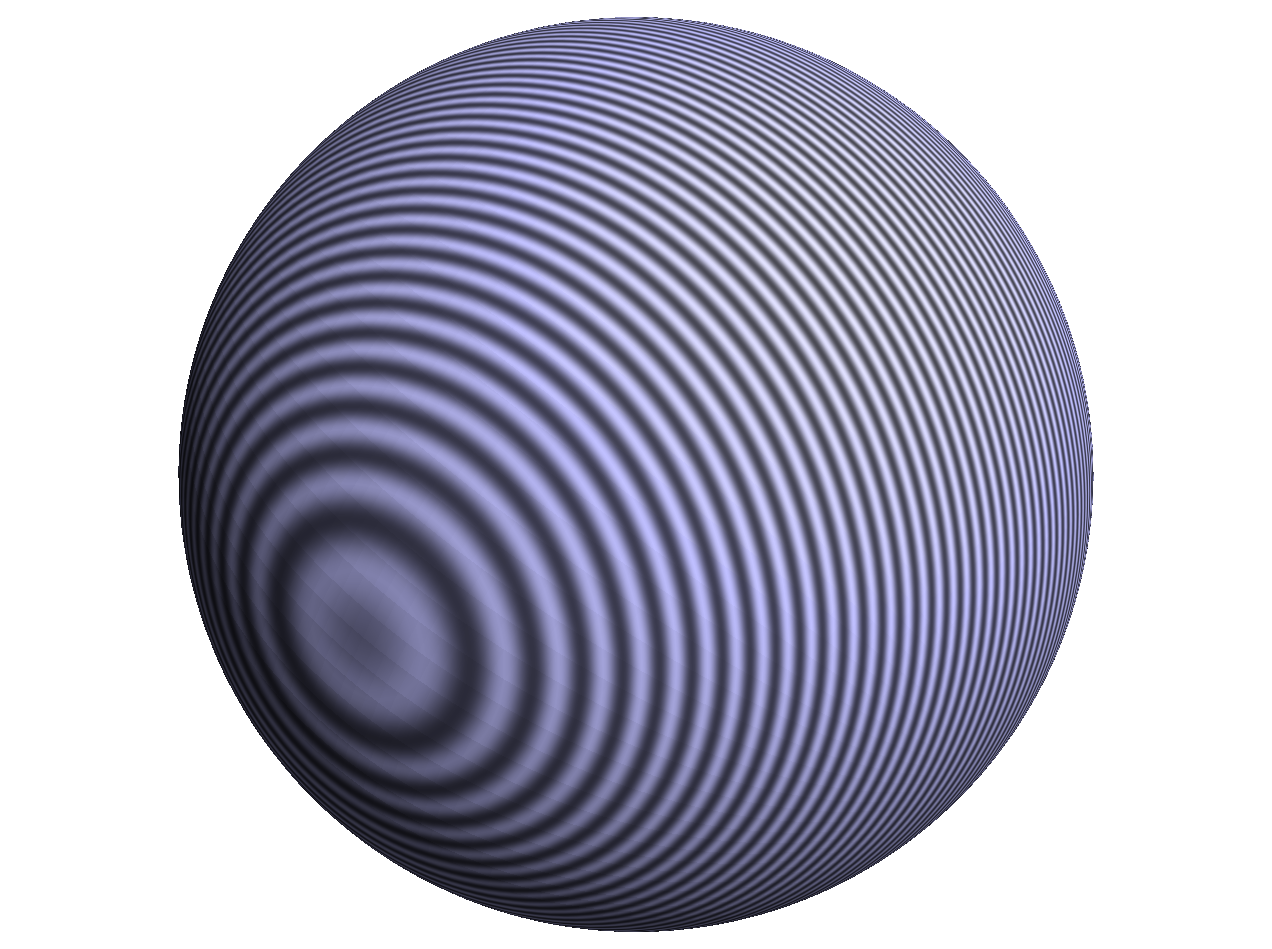
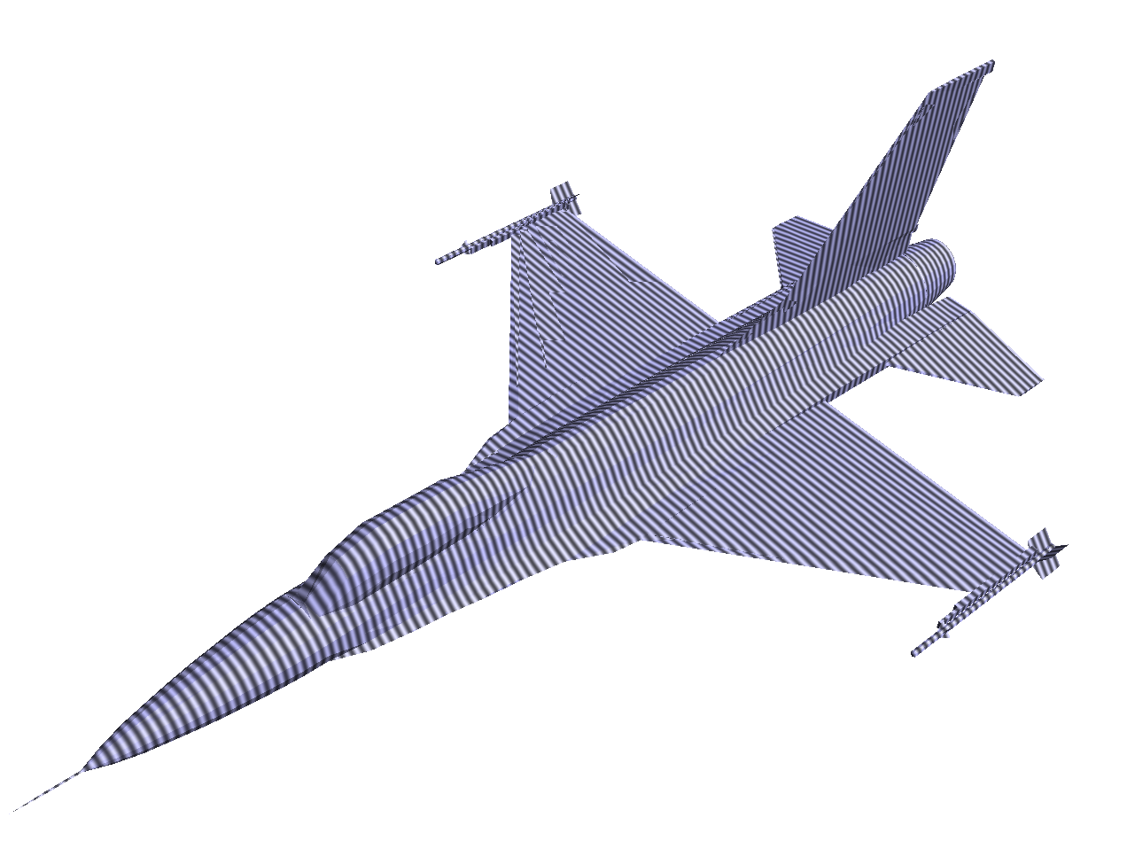
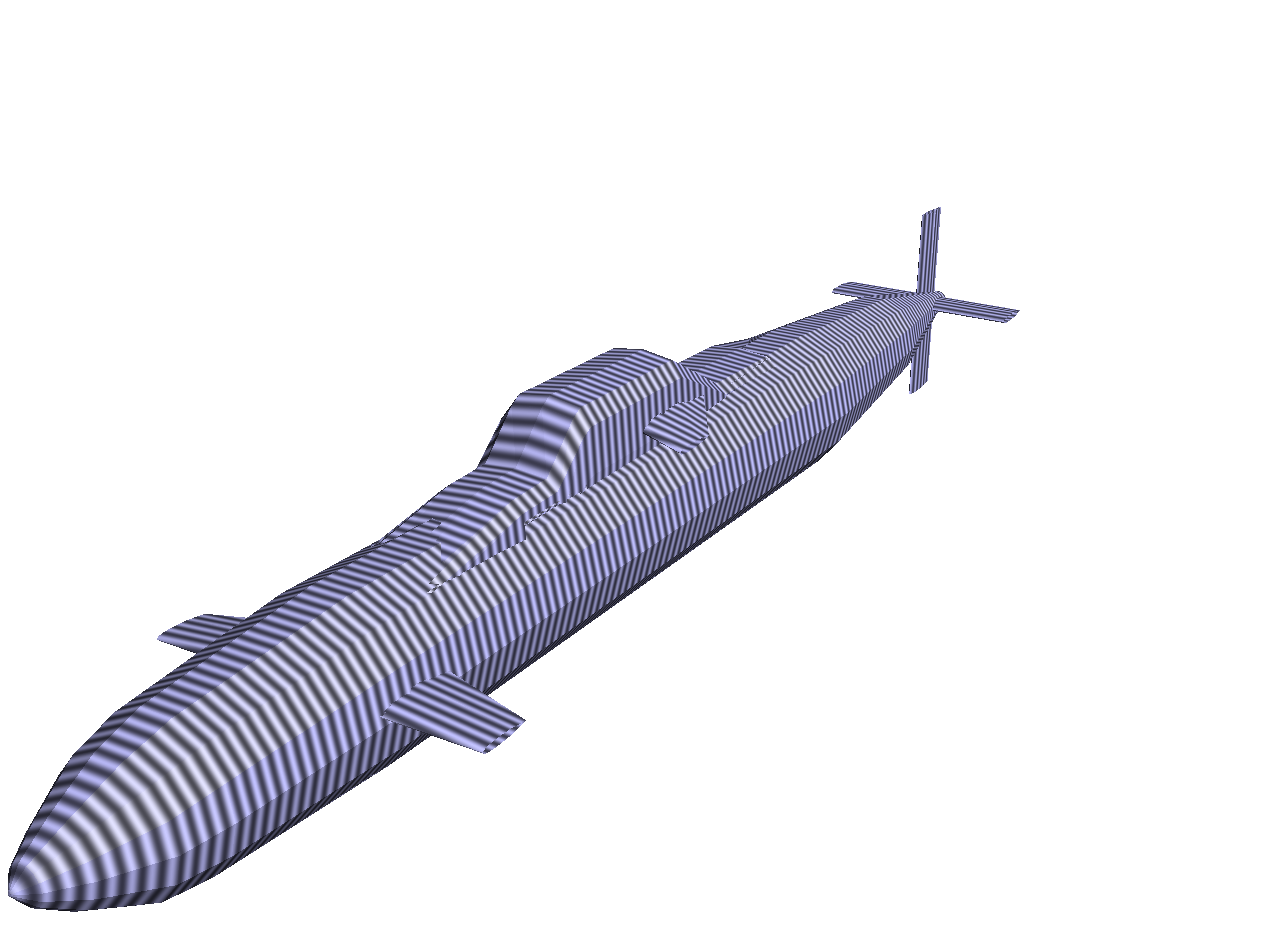
Fig. 5: Sphere (left), F16 (middle), and Submarine (right) geometries.

We test our algorithm on three geometries: a sphere, an F16 fighter aircraft, and a submarine. The geometries are in Figure 5. The surface of each geometry is represented by a triangular mesh, and the point set $\{p_{i}\}$ is generated by sampling the triangular mesh randomly with $10$ points per wavelength on average. The densities $\{f_{i}\}$ are generated by independently sampling from a standard normal distribution.

In our experiments, we use simple clustering techniques to partition the data and create the partition $\mathcal{P}$. To partition the points, we use k-means clustering, ignoring the octree boxes where the points live. To create $\mathcal{P}$, we use an algorithm that greedily assigns a box to the process that owns the most points in the box while also balancing the number of boxes on each process. Algorithm 3 formally describes the construction of $\mathcal{P}$. Because the points are partitioned with k-means clustering, Algorithm 3 outputs a map $\mathcal{P}$ that tends to cluster the assignment of process to box as well.

Result: partition $\mathcal{P}$

Compute $B_{max}=\lceil\#\left(\text{non-empty boxes at partition level}\right)/p\rceil$

$C=\{0,1,\ldots,p-1\}$

for $i=0$ to $p-1$ do

       $B_{i}=0$

foreach non-empty box $B$ at level $l_{p}$ do

       $i=\arg\max_{j\in C}\left|\{p_{k}\in B|p_{k}\text{ on process }j\}\right|$

       $\mathcal{P}(B)=i$

       $B_{i}=B_{i}+1$

       if $B_{i}==B_{max}$ then

             $C=C\backslash\{i\}$

      

Algorithm 3 Construction of $\mathcal{P}$ used in numerical experiments.

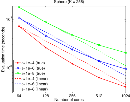
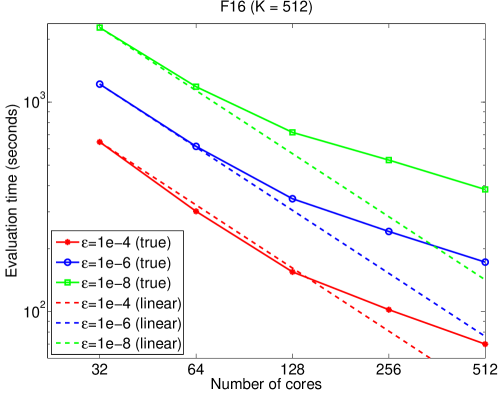
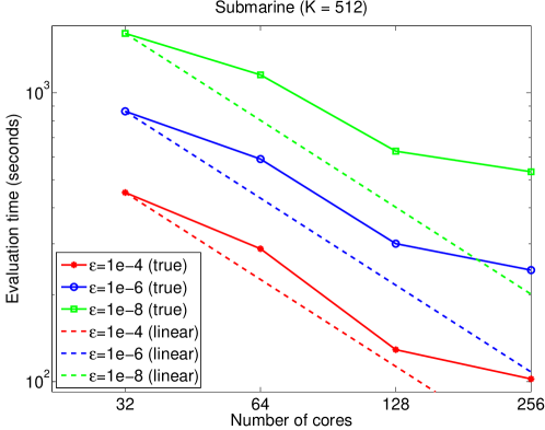
Fig. 6: Weak scaling experiments for Sphere ($K=256$), F16 ($K=512$), and Submarine ($K=512$). Dashed lines are linear scaling from the running time with the smallest number of cores.

Table 3: Number of non-empty boxes at the partition level $l_{p}$. As discussed in subsection 3.6, this limits scalability. In all numerical experiments for all geometries, $l_{p}=5$.

Geometry	#(non-empty boxes)	#(boxes)
Sphere	2,136	32,768
F16	342	32,768
Submarine	176	32768

Figure 6 shows strong scaling results for the algorithm on the geometries with target accuracy $\epsilon=$1e-4, 1e-6, and 1e-8. The smallest number of cores used for each geometry is chosen as the smallest power of two such that the algorithm does not run out of memory when $\epsilon=$ 1e-8. Our algorithm scales best for the sphere geometry. This makes sense because the symmetry of the geometry balances the number of directions assigned to each process. While we use a power-of-two number of processes in the scaling experiments, we note that our implementation works for an arbitrary number of processes.

Scaling levels off at 512 cores for the F16 and 256 cores for the Submarine. This is a direct consequence of the number of non-empty boxes in the octree at the partition level, which was discussed in subsection 3.6. Table 3 lists the number of nonempty boxes for the three geometries.

Table 4: Breakdown of running times for the parallel algorithm. All listed times are in seconds. For all geometries, the more accurate solutions produce worse scalings

Geometry (K)	$\epsilon$	p	HF-M2M	HF-M2L	LF-M2L	HF+LF	Total	Efficiency
				+ HF-L2L	+ LF-L2L	Comm.
Sphere (256)	1e-4	64	29.44	525.69	159.83	5.53	722.73	100.0%
		128	17.76	187.88	50.85	2.77	261.55	138.16%
		256	12.1	88.7	17.54	1.96	121.32	148.93%
		512	8.83	45.75	6.19	0.97	62.47	144.61%
		1024	7.28	29.12	2.8	0.71	40.25	112.22%
Sphere (256)	1e-6	64	70.4	773.39	229.38	8.18	1084.9	100.0%
		128	43.21	334.31	73.89	4.39	458.11	118.41%
		256	30.57	177.5	26.6	2.16	238.92	113.52%
		512	23.0	102.91	10.1	1.31	138.3	98.05%
		1024	18.71	69.02	4.86	1.04	94.36	71.86%
Sphere (256)	1e-8	64	167.73	1293.32	284.51	21.24	1773.42	100.0%
		128	101.58	657.19	101.22	8.16	872.38	101.64%
		256	70.41	359.07	39.89	2.7	474.19	93.5%
		512	52.31	220.45	17.93	1.52	293.57	75.51%
		1024	42.28	150.04	9.33	1.2	204.67	54.15%
F16 (512)	1e-4	32	33.22	470.32	134.85	4.49	646.01	100.0%
		64	19.32	230.77	46.92	2.48	301.27	107.21%
		128	12.66	122.01	17.67	1.43	154.88	104.27%
		256	8.93	80.78	9.67	1.68	102.23	78.99%
		512	7.14	56.32	5.11	0.73	70.0	57.68%
F16 (512)	1e-6	32	84.26	895.07	229.44	5.25	1219.35	100.0%
		64	49.46	480.55	79.28	3.13	615.39	99.07%
		128	32.72	276.15	33.25	1.97	345.99	88.11%
		256	23.73	197.55	17.26	1.41	241.43	63.13%
		512	19.18	140.59	10.48	0.99	172.41	44.2%
F16 (512)	1e-8	32	195.51	1769.14	290.37	7.04	2271.94	100.0%
		64	118.07	944.96	112.72	4.25	1185.44	95.83%
		128	76.21	585.09	50.34	2.76	717.81	79.13%
		256	57.51	435.65	31.25	2.16	529.37	53.65%
		512	46.1	314.68	18.73	1.41	383.06	37.07%
Submarine (512)	1e-4	32	23.42	349.93	71.66	4.07	451.51	100.0%
		64	17.18	226.32	40.21	2.65	288.43	78.27%
		128	10.2	104.03	12.36	1.43	128.99	87.51%
		256	9.01	82.88	8.36	1.07	102.14	55.26%
Submarine (512)	1e-6	32	57.6	667.59	128.79	5.35	863.21	100.0%
		64	42.15	475.55	65.86	3.35	589.66	73.2%
		128	26.37	245.83	24.66	1.91	300.38	71.84%
		256	23.56	201.56	15.27	1.51	243.27	44.35%
Submarine (512)	1e-8	32	136.74	1281.87	172.27	8.09	1606.38	100.0%
		64	101.14	948.74	94.44	4.7	1154.14	69.59%
		128	61.57	523.28	37.73	2.66	628.12	63.94%
		256	55.03	447.74	25.8	2.01	532.93	37.68%

Table 4 provides a breakdown of the running times of the different components of the algorithm. We see the following trends in the data:

• The HF-M2L and HF-L2L (the downwards pass in the high-frequency regime) constitute the bulk of the running time. M2L is typically the most expensive translation operator [38], and the interaction lists are larger in the high-frequency regime than in the low-frequency regime.

• Communication time is small. The high-frequency and low-frequency communication combined are about 1% of the running time. For the number of processes in these experiments, this problem is expected to be compute bound. This agrees with studies on communication times in KI-FMM [11].

• The more accurate solutions do not scale as well as less accurate solutions. Higher accuracy solutions are more memory constrained, and we speculate that lower accuracy solutions benefit relatively more from cache effects when the number of cores increases.

The data show super-linear speedups for the sphere and F16 geometries at some accuracies. This is partly caused by the sub-optimality of the partitioning algorithm (Algorithm 3). However, the speedups are still encouraging.

5 Conclusion and future work

We have presented the first parallel algorithm for the directional multilevel approach for $N$-body problems with the Helmholtz kernel. Under proper load balancing, the computational complexity of the algorithm is $\mathcal{O}(N\log N/p)$, and the communication time is $\mathcal{O}(p\alpha+\frac{1}{p}N\log N\beta)$. Communication time is minimal in our experiments. The number of processes is limited to $\mathcal{O}(\sqrt{N})$, so the running time can essentially be reduced to $\mathcal{O}(\sqrt{N}\log N)$. The algorithm exhibits good strong scaling for a variety of geometries and target accuracies.

In future work, we plan to address the following issues:

• Partitioning the computation at a fixed level in the octree avoids communication at high levels in the octree but limits the parallelism. In future work, we plan to divide the work at lower levels of the octree and introduce more communication. Since communication is such a small part of the running time in our algorithm, it is reasonable to expect further improvements with these changes.

• Our algorithm uses $\mathcal{O}(w^{2})$ wedges for boxes of width $w$. This makes pre-computation expensive. We would like to reduce the total number of wedges at each box width.

• Our implementation uses a simple octree construction. We would like to incorporate the more sophisticated approaches of software such as p4est [7] and Dendro [28] in order to improve our parallel octree manipulations. This would alleviate memory constraints, since octree information is currently redundantly stored on each process.

References

- [1] G. Ballard, J. Demmel, O. Holtz, and O. Schwartz. Minimizing communication in numerical linear algebra. SIAM Journal on Matrix Analysis and Applications, 32(3):866–901, 2011.
- [2] E. Bleszynski, M. Bleszynski, and T. Jaroszewicz. AIM: Adaptive integral method for solving large-scale electromagnetic scattering and radiation problems. Radio Science, 31(5):1225–1251, 1996.
- [3] N. N. Bojarski. K-space formulation of the electromagnetic scattering problem. Technical report, DTIC Document, 1972.
- [4] B. Bradie, R. Coifman, and A. Grossmann. Fast numerical computations of oscillatory integrals related to acoustic scattering, I. Applied and Computational Harmonic Analysis, 1(1):94–99, 1993.
- [5] J. Bruck, C.-T. Ho, S. Kipnis, E. Upfal, and D. Weathersby. Efficient algorithms for all-to-all communications in multiport message-passing systems. Parallel and Distributed Systems, IEEE Transactions on, 8(11):1143–1156, 1997.
- [6] O. P. Bruno and L. A. Kunyansky. A fast, high-order algorithm for the solution of surface scattering problems: basic implementation, tests, and applications. Journal of Computational Physics, 169(1):80–110, 2001.
- [7] C. Burstedde, L. C. Wilcox, and O. Ghattas. p4est: Scalable algorithms for parallel adaptive mesh refinement on forests of octrees. SIAM Journal on Scientific Computing, 33(3):1103–1133, 2011.
- [8] F. X. Canning. Sparse approximation for solving integral equations with oscillatory kernels. SIAM Journal on Scientific and Statistical Computing, 13(1):71–87, 1992.
- [9] C. Cecka and E. Darve. Fourier-based fast multipole method for the Helmholtz equation. SIAM Journal on Scientific Computing, 35(1):A79–A103, 2013.
- [10] E. Chan, M. Heimlich, A. Purkayastha, and R. Van De Geijn. Collective communication: theory, practice, and experience. Concurrency and Computation: Practice and Experience, 19(13):1749–1783, 2007.
- [11] A. Chandramowlishwaran, J. Choi, K. Madduri, and R. Vuduc. Brief announcement: towards a communication optimal fast multipole method and its implications at exascale. In Proceedinbgs of the 24th ACM symposium on Parallelism in algorithms and architectures, pages 182–184. ACM, 2012.
- [12] A. Chandramowlishwaran, S. Williams, L. Oliker, I. Lashuk, G. Biros, and R. Vuduc. Optimizing and tuning the fast multipole method for state-of-the-art multicore architectures. In Parallel & Distributed Processing (IPDPS), 2010 IEEE International Symposium on, pages 1–12. IEEE, 2010.
- [13] H. Cheng, W. Y. Crutchfield, Z. Gimbutas, L. F. Greengard, J. F. Ethridge, J. Huang, V. Rokhlin, N. Yarvin, and J. Zhao. A wideband fast multipole method for the Helmholtz equation in three dimensions. Journal of Computational Physics, 216(1):300–325, 2006.
- [14] H. Cheng, L. Greengard, and V. Rokhlin. A fast adaptive multipole algorithm in three dimensions. Journal of Computational Physics, 155(2):468–498, 1999.
- [15] W. C. Chew, E. Michielssen, J. Song, and J. Jin. Fast and efficient algorithms in computational electromagnetics. Artech House, Inc., 2001.
- [16] D. L. Colton and R. Kress. Inverse acoustic and electromagnetic scattering theory, volume 93. Springer, 2013.
- [17] E. Darve, C. Cecka, and T. Takahashi. The fast multipole method on parallel clusters, multicore processors, and graphics processing units. Comptes Rendus Mècanique, 339(2–3):185 – 193, 2011. High Performance Computing.
- [18] B. Engquist and L. Ying. Fast directional multilevel algorithms for oscillatory kernels. SIAM Journal on Scientific Computing, 29(4):1710–1737, 2007.
- [19] B. Engquist and L. Ying. A fast directional algorithm for high frequency acoustic scattering in two dimensions. Communications in Mathematical Sciences, 7(2):327–345, 2009.
- [20] B. Engquist and L. Ying. Fast directional algorithms for the Helmholtz kernel. J. Comput. Appl. Math., 234(6):1851–1859, July 2010.
- [21] O. Ergul and L. Gurel. Efficient parallelization of the multilevel fast multipole algorithm for the solution of large-scale scattering problems. Antennas and Propagation, IEEE Transactions on, 56(8):2335–2345, 2008.
- [22] O. Ergul and L. Gurel. A hierarchical partitioning strategy for an efficient parallelization of the multilevel fast multipole algorithm. Antennas and Propagation, IEEE Transactions on, 57(6):1740–1750, 2009.
- [23] L. Greengard and W. Gropp. A parallel version of the fast multipole method. Computers & Mathematics with Applications, 20(7):63 – 71, 1990.
- [24] J. G. Harris. Linear elastic waves, volume 26. Cambridge University Press, 2001.
- [25] J. MacQueen et al. Some methods for classification and analysis of multivariate observations. In Proceedings of the fifth Berkeley symposium on mathematical statistics and probability, volume 1, page 14. California, USA, 1967.
- [26] A. Rahimian, I. Lashuk, S. Veerapaneni, A. Chandramowlishwaran, D. Malhotra, L. Moon, R. Sampath, A. Shringarpure, J. Vetter, R. Vuduc, et al. Petascale direct numerical simulation of blood flow on 200k cores and heterogeneous architectures. In Proceedings of the 2010 ACM/IEEE International Conference for High Performance Computing, Networking, Storage and Analysis, pages 1–11. IEEE Computer Society, 2010.
- [27] V. Rokhlin. Diagonal forms of translation operators for Helmholtz equation in three dimensions. Technical report, DTIC Document, 1992.
- [28] R. S. Sampath, S. S. Adavani, H. Sundar, I. Lashuk, and G. Biros. Dendro: parallel algorithms for multigrid and AMR methods on 2:1 balanced octrees. In Proceedings of the 2008 ACM/IEEE conference on Supercomputing, page 18. IEEE Press, 2008.
- [29] J. Song and W. C. Chew. Multilevel fast-multipole algorithm for solving combined field integral equations of electromagnetic scattering. Microwave and Optical Technology Letters, 10(1):14–19, 1995.
- [30] J. Song, C.-C. Lu, and W. C. Chew. Multilevel fast multipole algorithm for electromagnetic scattering by large complex objects. Antennas and Propagation, IEEE Transactions on, 45(10):1488–1493, 1997.
- [31] J. M. Taboada, M. G. Araujo, J. M. Bertolo, L. Landesa, F. Obelleiro, and J. L. Rodriguez. MLFMA-FFT parallel algorithm for the solution of large-scale problems in electromagnetics. Progress In Electromagnetics Research, 105:15–30, 2010.
- [32] R. Thakur, R. Rabenseifner, and W. Gropp. Optimization of collective communication operations in MPICH. International Journal of High Performance Computing Applications, 19(1):49–66, 2005.
- [33] K. D. Tran. Fast numerical methods for high frequency wave scattering. PhD thesis, University of Texas at Austin, 2012.
- [34] P. Tsuji and L. Ying. A fast directional algorithm for high-frequency electromagnetic scattering. Journal of Computational Physics, 230(14):5471–5487, 2011.
- [35] C. Waltz, K. Sertel, M. A. Carr, B. C. Usner, and J. L. Volakis. Massively parallel fast multipole method solutions of large electromagnetic scattering problems. Antennas and Propagation, IEEE Transactions on, 55(6):1810–1816, 2007.
- [36] L. Ying. Fast algorithms for boundary integral equations. In Multiscale Modeling and Simulation in Science, pages 139–193. Springer, 2009.
- [37] L. Ying, G. Biros, and D. Zorin. A kernel-independent adaptive fast multipole algorithm in two and three dimensions. Journal of Computational Physics, 196(2):591–626, 2004.
- [38] L. Ying, G. Biros, D. Zorin, and H. Langston. A new parallel kernel-independent fast multipole method. In Supercomputing, 2003 ACM/IEEE Conference, pages 14–14. IEEE, 2003.
- [39] R. Yokota and L. Barba. Hierarchical n-body simulations with autotuning for heterogeneous systems. Computing in Science & Engineering, 14(3):30–39, 2012.
- [40] R. Yokota and L. A. Barba. A tuned and scalable fast multipole method as a preeminent algorithm for exascale systems. International Journal of High Performance Computing Applications, 26(4):337–346, 2012.