Sparse Identification of Posynomial Models

Abstract

Posynomials are nonnegative combinations of monomials with possibly fractional and both positive and negative exponents. Posynomial models are widely used in various engineering design endeavors, such as circuits, aerospace and structural design, mainly due to the fact that design problems cast in terms of posynomial objectives and constraints can be solved efficiently by means of a convex optimization technique known as geometric programming (GP). However, while quite a vast literature exists on GP-based design, very few contributions can yet be found on the problem of identifying posynomial models from experimental data. Posynomial identification amounts to determining not only the coefficients of the combination, but also the exponents in the monomials, which renders the identification problem numerically hard. In this draft, we propose an approach to the identification of multivariate posynomial models, based on the expansion on a given large-scale basis of monomials. The model is then identified by seeking coefficients of the combination that minimize a mixed objective, composed by a term representing the fitting error and a term inducing sparsity in the representation, which results in a problem formulation of the “square-root LASSO” type, with nonnegativity constraints on the variables. We propose to solve the problem via a sequential coordinate-descent scheme, which is suitable for large-scale implementations.

Key Words: Posynomial models, Identification, Sparse optimization, Square-root LASSO, Coordinate-descent methods.

1 Introduction

A posynomial model is defined by a function $\psi$ of the form

$$\psi(w)=\sum_{i=1}^{n_{c}}c_{i}w^{\alpha_{i}}$$ (1)

where $w\in\mathbb{R}_{++}^{n_{w}}$ (the positive orthant), $\psi(w)\in\mathbb{R}$, $c_{i}\geq 0$ are coefficients, $\alpha_{i}=[\alpha_{i1}\,\cdots\,\alpha_{in_{w}}]^{\top}\in\mathbb{R}^{n_{w}}$ are vectors of exponents with $\alpha_{ij}\in\mathbb{R}$, and $w^{\alpha_{i}}$ is defined as

$$w^{\alpha_{i}}\doteq\prod_{j=1}^{n_{w}}w_{j}^{\alpha_{ij}}.$$

The term $c_{i}w^{\alpha_{i}}$ is called a monomial. Note that, while in polynomial models the exponents $\alpha_{ij}$ are nonnegative integers, in posynomial models these exponents may also be negative and/or noninteger.

Posynomial models are of great importance in many fields of technology, ranging from structural design, network flow, optimal control (see [2, 33]), to aerospace system design [14], circuit design [5, 8, 26], antennas [1] and communication systems [7]. The interest in posynomials is motivated by the fact that they lead to computationally efficient geometric programming models for optimal system design, see, e.g., [10, 2, 33].

Despite the fact that a consistent number of papers is available in the literature where posynomial models and geometric programming are used for design purposes, very few works can be found to date addressing the relevant problem of identifying a posynomial model from experimental data; see [8] for such an exception. Typically, the model is assumed known (i.e., the coefficients $c_{i}$ and the exponents $\alpha_{ij}$ are assumed known), and then it is processed by geometric programming to obtain an optimal design. However, in most real-world applications, the model is not known a priori, and has to be identified from experimental data.

Identification of posynomial models can be performed following the standard approach used for polynomials. In this approach, an heuristic search finalized at finding a viable model structure, i.e., a suitable set of exponent vectors $\left\{\alpha_{i}\right\}$ is first carried out. Once the exponent vector set has been chosen, the coefficients $c_{i}$ are estimated by means of least-squares or other convex optimization algorithms, see, e.g., [29, 24, 8]. A critical issue in this approach is that the model structure search may be extremely time consuming and in most cases leads only to approximate model structures, see [21]. An alternative approach is to assume (or estimate by means of some heuristic) a value $\hat{n}_{c}$ for the basis cardinality $n_{c}$, and then estimate $c_{i}$ and $\alpha_{i}$ by means of nonlinear programming algorithms. However, these kind of algorithms are non-convex and thus do not ensure convergence to the optimal parameter estimate. A third approach, which overcomes the issues of the other two, consists in considering an over-parametrized model and inserting in the optimization problem a sparsity promoting term (or constraint), given by the $\ell_{1}$-norm of the coefficient vector. This term allows one to efficiently select the model structure and, at the same time, to avoid the problem of overfitting. This approach is based on the well-known LASSO (least absolute shrinkage and selection operator) or other similar algorithms (see, e.g., [30, 16, 3, 22] for applications of the approach to identification of polynomial models). The optimization problem is in this case convex but, due to the over-parametrization, it typically involves a very large number of decision variables.

In this paper, we follow this latter approach: we minimize a convex objective, defined as the sum of a regularized accuracy term based on the $\ell_{2}$-norm of the estimation residual, and a sparsity-inducing term given by a weighted $\ell_{1}$-norm of the coefficient vector. We name this approach nonnegative regularized square-root LASSO or nnrsqrt-LASSO, since it is similar to LASSO but presents three differences which may give advantages in terms of computational efficiency and model regularity. The first one is to use in the objective function an accuracy objective that is the square-root of the one used in LASSO. With this choice, we obtain an a-priori and easily checkable sufficient condition that, if satisfied for a certain monomial, guarantees that that monomial will not appear in the representation (i.e., it has a null coefficient). This condition (called feature elimination condition) can be verified very efficiently, and can thus be used in a pre-optimization phase to eliminate all the monomials which have very low relevance in explaining the data. The second difference is to include an $\ell_{2}$ regularization in the accuracy term, allowing us to implicitly account for uncertainty in the data, and to improve the numerical conditioning of the problem. The third difference consists in using a weighted $\ell_{1}$-norm of the coefficient vector in place of the standard $\ell_{1}$-norm. This allows for more flexibility in problems where the entries of $c$ have different scales. Note that in the nnrsqrt-LASSO the variables are constrained to be nonnegative, as required for the identification of posynomial models.

In order to solve the nnrsqrt-LASSO problem, we propose a large-scale-capable iterative algorithm based on sequential coordinate descent.

The remainder of the paper is organized as follows. In Section 2, the problem of identifying a posynomial model is introduced and then formulated in terms of a nnrsqrt-LASSO optimization problem. In Section 3, the dual formulation of this optimization problem is developed and the feature elimination condition is derived. Section 4 shows how the univariate nnrsqrt-LASSO optimization problem can be solved in closed form. Based on this result, in Section 5, a sequential coordinate descent scheme is proposed, allowing us to solve the multivariate optimization problem. The computational aspects of the proposed scheme are also discussed in this section. Finally, in Section 6, two numerical examples are presented. The first one regards identification of a posynomial with negative and non integer exponents; the second one is about identification of a posynomial model for a NACA 4412 airfoil.

2 Identification of posynomial models

2.1 Model setup

Consider a posynomial

$$\psi^{o}(w)=\sum_{i=1}^{n_{c}}c_{i}^{o}w^{\alpha_{i}^{o}}$$ (2)

where the coefficients $c_{i}^{o}$, the exponent vectors $\alpha_{i}^{o}$ and the expansion cardinality $n_{c}$ are not known. Suppose that a set of noise-corrupted measurements is available:

$$\mathfrak{D}=\left\{y(k),w(k)\right\}_{k=1}^{m}$$

where

$$y(k)=\psi^{o}(w(k))+e(k)$$

and $e(k)\in\mathbb{R}$ is a noise term. The problem considered in this paper is to estimate from these data the unknown parameters $c_{i}^{o}$, $\alpha_{i}^{o}$, $i=1,\ldots,n_{c}$, and the cardinality $n_{c}$.

To this end, we define an over-parametrized posynomial family

$$\psi(w)=\sum_{i=1}^{n}x_{i}w^{\alpha_{i}}$$ (3)

where $n\gg n_{c}$. In real-world situations, this over-parametrization can be obtained from the available prior information on the exponents $\alpha_{ij}^{o}$. For example, a certain exponent may be unknown but it can be known to be integer and to belong to a given interval; another one may be known to be fractional in another interval; another one can be known to be negative, etc.

More formally, suppose that the following prior information is available on the exponents:

$$\alpha_{ij}\in Q_{j}$$ (4)

where $Q_{j}$ is a set of exponents which, on the basis of the available prior information, can be considered reasonable for the variable $w_{j}$. Then, the set of exponent vectors defining the over-parametrization (3) can be constructed as

$$S_{\alpha}\doteq\left\{\alpha_{i}\right\}_{i=1}^{n}=\prod_{j=1}^{n_{w}}Q_{j}$$

where $\prod$ denotes the Cartesian product. Note that this approach can be adopted also if an exponent is known to belong to a continuous (finite) interval, in which case the set $Q_{j}$ can be obtained by properly discretizing the interval.

If the information (4) is correct, then $S_{\alpha}$ is guaranteed to contain the true exponent vectors:

$$S_{\alpha}\supset S_{\alpha^{o}}\doteq\left\{\alpha_{i}^{o}\right\}_{i=1}^{n_{c}}.$$

2.2 Square-root LASSO formulation of the identification problem

Model identification is here performed by minimizing with respect to the coefficients $x_{i}$ in the expansion (3) an objective function defined as the sum of an accuracy objective and a sparsity-promoting term, allowing us to select, in the over-parametrized family, a parsimonious model structure. Define $y=[y(1)\,\cdots\,y(m)]^{\top}$, $x=[x_{1}\,\cdots\,x_{n}]^{\top}$, and

$$\Phi=\left[\begin{array}[]{ccc}w(1)^{\alpha_{1}}&\cdots&w(1)^{\alpha_{n_{w}}}\\ \vdots&\ddots&\vdots\\ w(m)^{\alpha_{1}}&\cdots&w(m)^{\alpha_{n_{w}}}\end{array}\right].$$

The objective we consider is of the form

$$f(x)\doteq\left\|\left[\begin{array}[]{c}\Phi x-y\\ \sigma x\end{array}\right]\right\|_{2}+\lambda^{\top}\left|x\right|,$$ (5)

where $\sigma\geq 0$, $\lambda\in\mathbb{R}^{n}$ with $\lambda\geq 0$ (component-wise), and $|x|$ denotes a vector whose entries are the absolute values of the entries in $x$. We define, for notational compactness,

$$\tilde{\Phi}\doteq\left[\begin{array}[]{c}\Phi\\ \sigma I\end{array}\right],\quad\tilde{y}\doteq\left[\begin{array}[]{c}y\\ 0\end{array}\right],\quad\tilde{\phi}_{i}\doteq\left[\begin{array}[]{c}\phi_{i}\\ \sigma e_{i}\end{array}\right],$$

where $\tilde{\phi}_{i}$, $i=1,\ldots,n$, denotes the $i$-th column of $\tilde{\Phi}$, and $e_{i}$ is the $i$-th vector of the standard basis of $\mathbb{R}^{n}$. The objective thus becomes

$$f(x)\doteq\|\tilde{\Phi}x-\tilde{y}\|_{2}+\lambda^{\top}\left|x\right|.$$ (6)

Note that $\lambda^{\top}\left|x\right|$ is a weighted $\ell_{1}$-norm. Vector $\lambda$ is thus a penalty factor which quantifies the tradeoff between the accuracy objective $\|\tilde{\Phi}x-\tilde{y}\|_{2}$ and the term $\lambda^{\top}\left|x\right|$, which is a proxy for sparsity in the solution, see [13, 31, 9, 6]. Clearly, for $\lambda=\gamma{\mathbf{1}}$ (where ${\mathbf{1}}$ is a vector with all entries equal to one), and $\sigma=0$, the rsqrt-LASSO problem coincides with the standard sqrt-LASSO. The use of the sparsity promoting term $\lambda^{\top}\left|x\right|$ instead of the standard term $\gamma\|x\|_{1}$ allows for more flexibility, in problems where the entries of $x$ have different scales. The regularization parameter $\sigma\geq 0$ is introduced to improve the numerical conditioning of the problem, guaranteeing (if $\sigma>0$) that $\tilde{\Phi}$ has full rank, and that the $\ell_{2}$ term of the objective remains differentiable for all $x$.

We hence consider the following two optimization problems, which we name regularized square-root LASSO (rsqrt-LASSO)

$$p^{*}\doteq\min_{x\in\mathbb{R}^{n}}f(x),$$ (7)

and nonnegative regularized square-root LASSO (nnrsqrt-LASSO)

$$p_{+}^{*}\doteq\min_{x\in\mathbb{R}_{+}^{n}}f(x),$$ (8)

where $\mathbb{R}_{+}^{n}\doteq\{x\in\mathbb{R}^{n}:x\geq 0\}$ (the inequality is component-wise). The first model can be used for polynomial model identification, and the second one for posynomial model identification (the focus in this paper is on this latter case).

As already mentioned, the solutions of the optimization problems (7) and (8) tend to be sparse, i.e., to have only a few non-zero components. This important feature is produced by the $\ell_{1}$ term, which is able to select among the large set of monomials only those which are relevant to explain the data. Indeed, the $\ell_{1}$-norm is the convex envelope of the $\ell_{0}$ quasi-norm, a quantity defined as the number of vector non-zero elements, which is commonly used to measure vector sparsity. Minimizing the $\ell_{1}$-norm allows one to approximately minimize the $\ell_{0}$ quasi-norm, and thus to maximize the coefficient sparsity [13, 31, 9, 6]. While the $\ell_{0}$ quasi-norm is non-convex and its minimization is a NP-hard problem, the $\ell_{1}$-norm is convex and its minimization can be performed quite efficiently. Conditions under which the $\ell_{1}$ minimization problem provides a maximally sparse solution, i.e., a solution of the corresponding $\ell_{0}$ minimization problem, are given, e.g., in [22]. Note that the sparsity property is important also to allow an efficient implementation on real-time processors, which may have limited memory and computational capacity [23].

Remark 1

Notice that the cardinality $n$ of the set $S_{\alpha}$, and hence the dimension of the decision vector $x$, may be very large, since it is given by the product of the cardinalities of $Q_{j}$, for $j=1,\ldots,n_{w}$. For this reason, although the two previous problems are standard convex optimization problems, they may not be practically solved using standard interior-point methods for convex optimization. Actually, in some cases, even just storing in memory the data matrix $\Phi$ may be unfeasible due to dimensionality issues. $\square$

In the following sections, we describe a simple scheme for solving both the unconstrained and the constrained versions of the regularized sqrt-LASSO problem, based on a two-phase procedure. In the first phase, we apply a feature elimination step to eliminate a-priori all variables that are guaranteed to be zero at optimum, thus possibly reducing the dimensionality of the problem. In the second phase, we apply a coordinate-descent scheme to the reduced problem, in order to find the optimal solution. This latter phase is based on the fact that we can find in “closed form” an optimal solution to the univariate restriction of the above problems.

We shall assume throughout that $y\neq 0$, since for $y=0$ the optimal solution of both problems (7), (8) is trivially $x^{*}=0$.

3 Dual formulations and feature elimination

We next derive dual formulations of the rsqrt-LASSO and nnrsqrt-LASSO problems, and then show how a feature elimination condition is obtained from these dual formulations.

3.1 Dual of the rsqrt-LASSO problem

We here derive a dual formulation for problem (7). To this end, we first recall the definition of dual norm: if $\|\cdot\|$ is a vector norm, then the corresponding dual norm is defined as

$$\|x\|_{\star}\doteq\max_{\|v\|\leq 1}\,v^{\top}x.$$

It is well known, for instance, that the dual of the $\ell_{2}$ norm is the $\ell_{2}$ norm itself, and that the dual of the $\ell_{\infty}$ norm is the $\ell_{1}$ norm, and vice versa. Therefore,

$$\|\tilde{\Phi}x-\tilde{y}\|_{2} = \max_{\|u\|_{2}\leq 1}\,u^{\top}(\tilde{\Phi}x-\tilde{y}).$$

Also, one can readily verify that

$$\lambda^{\top}|x|=\sum_{i=1}^{n}\lambda_{i}|x_{i}|=\max_{|v|\leq\lambda}\,v^{\top}x.$$

We can thus rewrite problem (7) as

$$p^{*}=\min_{x\in{{\mathbb{R}}^{n}}} \displaystyle{\max_{\|u\|_{2}\leq 1,|v|\leq\lambda}}\;u^{\top}(\tilde{\Phi}x-\tilde{y})+v^{\top}x.$$

Then, a standard saddle-point result (see, for instance, Sion’s theorem, [15, 28]), prescribes that we may exchange the order of min and max in the previous expression without changing the optimal value, whence

$$p^{*} = \displaystyle{\max_{\|u\|_{2}\leq 1,|v|\leq\lambda}}\;\displaystyle{\min_{x\in{{\mathbb{R}}^{n}}}}\;u^{\top}(\tilde{\Phi}x-\tilde{y})+v^{\top}x.$$

Notice further that the infimum over $x\in{{\mathbb{R}}^{n}}$ of the term $(u^{\top}\tilde{\Phi}+v^{\top})x$ is $-\infty$, unless the coefficient $u^{\top}\tilde{\Phi}+v^{\top}$ is zero, hence

$$p^{*}=\displaystyle{\max_{u,v}} -u^{\top}\tilde{y}$$

s.t.: $$\tilde{\Phi}^{\top}u+v=0$$

$$\|u\|_{2}\leq 1$$

$$|v|\leq\lambda.$$

Eliminating the $v$ variable, we obtain the following formulation for the dual of problem (7)

$$p^{*}=\displaystyle{\max_{u}} -u^{\top}\tilde{y}$$ (9)

s.t.: $$\|u\|_{2}\leq 1$$ (10)

$$|\tilde{\phi}_{i}^{\top}u|\leq\lambda_{i}, i=1,\ldots,n.$$

3.2 Dual of the nnrsqrt-LASSO problem

The derivation of the dual for the nnrsqrt-LASSO problem (8) follows similar lines, noticing that, for $x\geq 0$, we have $\lambda^{\top}|x|=\lambda^{\top}x$, hence

$$p^{*}_{+} = \displaystyle{\max_{\|u\|_{2}\leq 1}}\;\displaystyle{\min_{x\geq 0}}\;u^{\top}(\tilde{\Phi}x-\tilde{y})+\lambda^{\top}x,$$

and the infimum over $x\geq 0$ of the term $(u^{\top}\tilde{\Phi}+\lambda^{\top})x$ is $-\infty$, unless $u^{\top}\tilde{\Phi}+\lambda^{\top}\geq 0$, thus

$$p^{*}_{+}=\displaystyle{\max_{u}} -u^{\top}\tilde{y}$$ (11)

s.t.: $$\|u\|_{2}\leq 1$$ (12)

$$\tilde{\phi}_{i}^{\top}u+\lambda_{i}\geq 0, i=1,\ldots,n.$$

3.3 Safe feature elimination

In this section we analyze the dual formulations of problems (7), (8), in order to derive a simple sufficient condition that permits to predict when an entry $x_{i}$ is zero at optimum, and hence to eliminate a priori some features (i.e., columns of $\tilde{\Phi}$) from the problem. This type of condition, first introduced by [11] in the context of the standard LASSO problem, is named safe feature elimination. Observe that

$$\max_{\|u\|_{2}\leq 1}\,|\tilde{\phi}_{i}^{\top}u| = \|\tilde{\phi}_{i}\|_{2}=\left\|\left[\begin{array}[]{c}\phi_{i}\\ \sigma e_{i}\end{array}\right]\right\|_{2}.$$

Therefore, if for some $i\in\{1,\ldots,n\}$ it holds that

$$\left\|\left[\begin{array}[]{c}\phi_{i}\\ \sigma e_{i}\end{array}\right]\right\|_{2}^{2}=\|\phi_{i}\|_{2}^{2}+\sigma^{2}<\lambda_{i}^{2}$$

then the corresponding constraint in (10), as well as in (12), will certainly be satisfied with strict inequality, that is, it will be inactive at the optimum. This means that it can be safely eliminated from the dual optimization problem, without changing the optimal objective value. Defining

$${\mathcal{F}}(\lambda)\doteq\{i:\,\|\phi_{i}\|_{2}^{2}+\sigma^{2}\geq\lambda_{i}^{2},\;i=1,\ldots,n\},$$

we thus have that

$$p^{*}=\displaystyle{\max_{u}} -u^{\top}\tilde{y}$$ (14)

s.t.: $$\|u\|_{2}\leq 1$$

$$|\tilde{\phi}_{i}^{\top}u|\leq\lambda_{i}, i\in{\mathcal{F}}(\lambda),$$

which is the dual of the “reduced” primal problem

$$p^{*}=\min_{\xi} \|\tilde{\Phi}_{{\mathcal{F}}(\lambda)}\xi-\tilde{y}\|_{2}+\lambda^{\top}|\xi|,$$ (15)

where $\tilde{\Phi}_{{\mathcal{F}}(\lambda)}$ is a matrix containing by columns vectors $\tilde{\phi}_{i}$, $i\in{\mathcal{F}}(\lambda)$, and $\xi$ is a decision variable vector, having dimension equal to the cardinality of ${\mathcal{F}}(\lambda)$. In other words, the features $x_{i}$ in the primal problem (7) corresponding to indexes $i$ in the set ${\mathcal{E}}(\lambda)$ complementary to ${\mathcal{F}}(\lambda)$, defined as

$${\mathcal{E}}(\lambda)\doteq\{i:\,\|\phi_{i}\|_{2}^{2}+\sigma^{2}<\lambda_{i}^{2},\;i=1,\ldots,n\},$$

are certainly zero at the optimum, that is

$$\|\phi_{i}\|_{2}^{2}+\sigma^{2}<\lambda_{i}^{2}\quad\Rightarrow\quad x_{i}^{*}=0.$$ (16)

Similarly, we have that

$$p^{*}_{+}=\displaystyle{\max_{u}} -u^{\top}\tilde{y}$$ (17)

s.t.: $$\|u\|_{2}\leq 1$$

$$\tilde{\phi}_{i}^{\top}u+\lambda_{i}\geq 0, i\in{\mathcal{F}}(\lambda),$$

is the dual of the “reduced” primal problem

$$p^{*}_{+}=\min_{\xi\geq 0} \|\tilde{\Phi}_{{\mathcal{F}}(\lambda)}\xi-\tilde{y}\|_{2}+\lambda^{\top}|\xi|.$$ (18)

3.3.1 When is $x=0$ optimal?

Point $x=0$ is optimal for problem (7) if and only if $p^{*}=\|\tilde{y}\|_{2}$, which is equivalent to $u=-\tilde{y}/\|\tilde{y}\|_{2}$ being optimal (hence feasible) for the dual problem. This happens if and only if

$$|\tilde{\phi}_{i}^{\top}\tilde{y}|\leq\lambda_{i}{\|\tilde{y}\|_{2}},\quad i=1,\ldots,n,$$

that is, since $\tilde{\phi}_{i}^{\top}\tilde{y}=\phi_{i}^{\top}y$, $\|\tilde{y}\|_{2}=\|y\|_{2}$, if an only if

$$|\phi_{i}^{\top}y|\leq\lambda_{i}{\|y\|_{2}},\quad i=1,\ldots,n.$$

Similarly, point $x=0$ is optimal for problem (8) if and only if $p^{*}_{+}=\|\tilde{y}\|_{2}$, which is equivalent to $u=-\tilde{y}/\|\tilde{y}\|_{2}$ being optimal (hence feasible) for the dual problem, which happens if and only if

$$\tilde{\phi}_{i}^{\top}\tilde{y}\leq\lambda_{i}{\|\tilde{y}\|_{2}},\quad i=1,\ldots,n,$$

or, equivalently,

$$\phi_{i}^{\top}y\leq\lambda_{i}{\|y\|_{2}},\quad i=1,\ldots,n.$$

4 Univariate solution of rsqrt-LASSO and nnrsqrt-LASSO

Consider the following rsqrt-LASSO problem with a single scalar variable $x$:

$$\min_{x\in{{\mathbb{R}}}}\,f(x)\doteq\left\|\left[\begin{array}[]{c}\phi x-y\\ \sigma ex-\xi\end{array}\right]\right\|_{2}+\lambda|x|,$$

where $\lambda,\sigma\geq 0$, $\phi\in{{\mathbb{R}}^{m}},y\in{{\mathbb{R}}^{m}}$, $\xi\in{{\mathbb{R}}^{n}}$ are given, and $e$ is a vector of all zeros, except for an entry in generic position $i$, which is equal to one, and correspondingly we postulate that $\xi_{i}=0$, thus it holds that $e^{\top}\xi=0$. We set for convenience

$$\tilde{\phi}\doteq\left[\begin{array}[]{c}\phi\\ \sigma e\end{array}\right],\quad\tilde{y}\doteq\left[\begin{array}[]{c}y\\ \xi\end{array}\right].$$ (19)

Thus, the problem rewrites to

$$\min_{x\in{{\mathbb{R}}}}\,f(x)\doteq\|\tilde{\phi}x-\tilde{y}\|_{2}+\lambda|x|.$$ (20)

We assume that $\tilde{y}\neq 0$ and $\tilde{\phi}\neq 0$, otherwise the optimal solution is simply $x=0$. Let us define

$$x{{}_{\mathrm{ls}}}\doteq\frac{\tilde{\phi}^{\top}\tilde{y}}{\|\tilde{\phi}\|_{2}^{2}}=\frac{\phi^{\top}y}{\|\phi\|_{2}^{2}+\sigma^{2}},$$

which corresponds to the solution of the problem for $\lambda=0$. The following theorem holds.

Theorem 1

Consider problem (20), with $\tilde{y}\neq 0$, $\tilde{\phi}\neq 0$, $\lambda\geq 0$.

1. $x^{*}=0$ is an optimal solution for (20) if and only if

   $$|\tilde{\phi}^{\top}\tilde{y}|\leq\lambda\|\tilde{y}\|_{2}$$

   (notice, in particular, that if $\|\tilde{\phi}\|_{2}\leq\lambda$, then the above condition is certainly satisfied, hence $x^{*}=0$).

2. If $|\tilde{\phi}^{\top}\tilde{y}|>\lambda\|\tilde{y}\|_{2}$ (hence $\|\tilde{\phi}\|_{2}>\lambda$), then the optimal solution of (20) is given by

   $$x^{*}=x{{}_{\mathrm{ls}}}-{\mbox{\rm sgn}\,}(x{{}_{\mathrm{ls}}})\frac{\lambda}{\|\tilde{\phi}\|_{2}^{2}}\sqrt{\frac{\|\tilde{\phi}\|_{2}^{2}\|\tilde{y}\|_{2}^{2}-(\tilde{\phi}^{\top}\tilde{y})^{2}}{\|\tilde{\phi}\|_{2}^{2}-\lambda^{2}}}.$$ (21)

Proof. The problem is convex but nonsmooth, hence we write the optimality conditions in terms of the subdifferential of the objective:

$$0\in\partial f(x)=\partial\|\tilde{\phi}x-\tilde{y}\|_{2}+\lambda\partial|x|,$$

where

$$\partial\|\tilde{\phi}x-\tilde{y}\|_{2} = \left\{\displaystyle{\begin{array}[]{ll}\displaystyle{\frac{\tilde{\phi}^{\top}(\tilde{\phi}x-\tilde{y})}{\|\tilde{\phi}x-\tilde{y}\|_{2}}}&\mbox{if }\tilde{\phi}x-\tilde{y}\neq 0\\ \{\tilde{\phi}^{\top}g:\;\|g\|_{2}\leq 1\}&\mbox{if }\tilde{\phi}x-\tilde{y}=0,\end{array}}\right.$$

$$\partial|x| = \left\{\begin{array}[]{ll}{\mbox{\rm sgn}\,}(x)&\mbox{if }x\neq 0\\ \{v:\;|v|\leq 1\}&\mbox{if }x=0.\end{array}\right.$$

For point 1. we thus check under what conditions $0$ is contained in the subdifferential of $f$ at $x=0$, that is

$$\begin{array}[]{c}x^{*}=0\mbox{ is optimal}\\ \Updownarrow\\ 0\in\partial f(0)=\left\{\frac{\tilde{\phi}^{\top}\tilde{y}}{\|\tilde{y}\|_{2}}+\lambda v,\;|v|\leq 1\right\}.\end{array}$$

Since the term $\lambda v$ may take any value in the interval $[-\lambda,\,\lambda]$, it follows that the above condition is satisfied if and only if ${|\tilde{\phi}^{\top}\tilde{y}|}/{\|\tilde{y}\|_{2}}\leq\lambda$, which proves the first part of the theorem. Also, since by the Cauchy-Schwartz inequality it holds that

$$|\tilde{\phi}^{\top}\tilde{y}|\leq\|\tilde{\phi}\|_{2}\|\tilde{y}\|_{2},$$

it is clear that $\|\tilde{\phi}\|_{2}\leq\lambda$ implies $|\tilde{\phi}^{\top}\tilde{y}|\leq\lambda\|\tilde{y}\|_{2}$, hence the optimal solution is certainly zero when $\|\tilde{\phi}\|_{2}\leq\lambda$.

Consider next the case when the optimal solution is nonzero, i.e., when $|\tilde{\phi}^{\top}\tilde{y}|>\lambda\|\tilde{y}\|_{2}$, thus $\|\tilde{\phi}\|_{2}>\lambda$. We initially assume for simplicity that $\tilde{\phi}$ and $\tilde{y}$ are not collinear, so that $\tilde{\phi}x-\tilde{y}\neq 0$ for all $x$; later we show that the derived solution is still valid if this assumption is lifted. With this assumption, and since $x\neq 0$, we have that

$$x\mbox{ is optimal}\quad\Leftrightarrow\quad 0=\partial f(x)=\frac{\tilde{\phi}^{\top}(\tilde{\phi}x-\tilde{y})}{\|\tilde{\phi}x-\tilde{y}\|_{2}}+\lambda\,{\mbox{\rm sgn}\,}(x),$$

that is, since $\|\tilde{\phi}x-\tilde{y}\|_{2}\neq 0$, for

$$\tilde{\phi}^{\top}(\tilde{\phi}x-\tilde{y})=-\lambda\|\tilde{\phi}x-\tilde{y}\|_{2}{\mbox{\rm sgn}\,}(x).$$ (24)

All solution to this equation are also solutions of the squared equation

$$(\tilde{\phi}^{\top}\tilde{\phi}x-\tilde{\phi}^{\top}\tilde{y})^{2}=\lambda^{2}\|\tilde{\phi}x-\tilde{y}\|_{2}^{2},$$ (25)

which is a quadratic equation in $x$, equivalent to:

$$\|\tilde{\phi}\|_{2}^{2}(\|\tilde{\phi}\|_{2}^{2}-\lambda^{2})x^{2}-2\tilde{\phi}^{\top}\tilde{y}(\|\tilde{\phi}\|_{2}^{2}-\lambda^{2})x+(\tilde{\phi}^{\top}\tilde{y})^{2}-\lambda^{2}\|\tilde{y}\|_{2}^{2}=0.$$

The roots of this equation are in

$$x_{\pm}=x{{}_{\mathrm{ls}}}\pm\sqrt{x{{}_{\mathrm{ls}}}^{2}-\frac{(\tilde{\phi}^{\top}\tilde{y})^{2}-\lambda^{2}\|\tilde{y}\|_{2}^{2}}{\|\tilde{\phi}\|_{2}^{2}(\|\tilde{\phi}\|_{2}^{2}-\lambda^{2})}.}$$

Observe that the term under the square root is nonnegative, since

$$\delta\doteq x{{}_{\mathrm{ls}}}^{2}-\frac{(\tilde{\phi}^{\top}\tilde{y})^{2}-\lambda^{2}\|\tilde{y}\|_{2}^{2}}{\|\tilde{\phi}\|_{2}^{2}(\|\tilde{\phi}\|_{2}^{2}-\lambda^{2})} = \frac{(\tilde{\phi}^{\top}\tilde{y})^{2}}{\|\tilde{\phi}\|^{4}}-\frac{(\tilde{\phi}^{\top}\tilde{y})^{2}-\lambda^{2}\|\tilde{y}\|_{2}^{2}}{\|\tilde{\phi}\|_{2}^{2}(\|\tilde{\phi}\|_{2}^{2}-\lambda^{2})}$$

$$= \frac{\lambda^{2}}{\|\tilde{\phi}\|_{2}^{2}}\cdot\frac{\|\tilde{\phi}\|_{2}^{2}\|\tilde{y}\|_{2}^{2}-(\tilde{\phi}^{\top}\tilde{y})^{2}}{\|\tilde{\phi}\|_{2}^{2}(\|\tilde{\phi}\|_{2}^{2}-\lambda^{2})},$$

where, under the conditions of point 2., $\|\tilde{\phi}\|_{2}^{2}-\lambda^{2}>0$, and $\|\tilde{\phi}\|_{2}^{2}\|\tilde{y}\|_{2}^{2}-(\tilde{\phi}^{\top}\tilde{y})^{2}\geq 0$, by the Cauchy-Schwartz inequality. Further, $\delta\geq 0$ is smaller in magnitude than $x{{}_{\mathrm{ls}}}^{2}$, since the condition $|\tilde{\phi}^{\top}\tilde{y}|>\lambda\|\tilde{y}\|_{2}$ implies that $x{{}_{\mathrm{ls}}}^{2}-\delta>0$. It follows that the sign of $x_{\pm}=x{{}_{\mathrm{ls}}}\pm\sqrt{\delta}$ is the same sign of $x{{}_{\mathrm{ls}}}$ (since adding $\pm\sqrt{\delta}$ to $x{{}_{\mathrm{ls}}}$ cannot change its sign). Then, plugging $x\leftarrow x_{\pm}$ into equation (24), we have the left-hand side

$$\|\tilde{\phi}\|_{2}^{2}x_{\pm}-\tilde{\phi}^{\top}\tilde{y}=\|\tilde{\phi}\|_{2}^{2}(x{{}_{\mathrm{ls}}}\pm\sqrt{\delta})-\tilde{\phi}^{\top}\tilde{y}=\pm\sqrt{\delta}$$

and the right-hand side

$$-\lambda\|\tilde{\phi}x_{\pm}-\tilde{y}\|_{2}{\mbox{\rm sgn}\,}(x_{\pm})=-\lambda\|\tilde{\phi}x_{\pm}-\tilde{y}\|_{2}{\mbox{\rm sgn}\,}(x{{}_{\mathrm{ls}}}).$$

Thus, sign consistency is obtained by choosing the solution with “+” when $x{{}_{\mathrm{ls}}}$ is negative, and with “-” when $x{{}_{\mathrm{ls}}}$ is positive. In conclusion, the unique solution to eq. (24) is given by

$$x^{*}=x{{}_{\mathrm{ls}}}-{\mbox{\rm sgn}\,}(x{{}_{\mathrm{ls}}})\frac{\lambda}{\|\tilde{\phi}\|_{2}^{2}}\sqrt{\frac{\|\tilde{\phi}\|_{2}^{2}\|\tilde{y}\|_{2}^{2}-(\tilde{\phi}^{\top}\tilde{y})^{2}}{\|\tilde{\phi}\|_{2}^{2}-\lambda^{2}}},$$

which is the expression we wished to prove.

It only remains to be proved that the above expression is still valid also when $\tilde{y}$ and $\tilde{\phi}$ are collinear. In this case, since $\|\tilde{\phi}\|_{2}^{2}\|\tilde{y}\|_{2}^{2}=(\tilde{\phi}^{\top}\tilde{y})^{2}$, eq. (21) gives $x^{*}=x{{}_{\mathrm{ls}}}$, and we have that $\tilde{\phi}x^{*}-\tilde{y}=0$. Let us check that this solution is indeed optimal. The subdifferential of $f$ at $x^{*}\neq 0$ such that $\tilde{\phi}x^{*}-\tilde{y}=0$ is

$$\partial f(x^{*})=\{\tilde{\phi}^{\top}g+\lambda\,{\mbox{\rm sgn}\,}(x^{*}),\;\|g\|_{2}\leq 1\},$$

and we see that $0\in\partial f(x^{*})$ if $\|\tilde{\phi}\|_{2}\geq\lambda$, which is indeed the condition under which the expression (21) for $x^{*}$ holds. $\square$

4.1 Univariate solution of nnrsqrt-LASSO

The solution of the univariate nnrsqrt-LASSO problem in the scalar variable $x$

$$\min_{x\geq 0}\,f(x)\doteq\|\tilde{\phi}x-\tilde{y}\|_{2}+\lambda|x|,$$ (26)

can be readily obtained from the solution of the corresponding unconstrained problem (20), by the following reasoning. Since (26) is a convex optimization problem in one variable and one linear inequality constraint, its optimal solution is either on the boundary of the feasible set (in this case, at $x=0$), or it coincides with the solution of the unconstrained version of the problem. Thus, we solve the unconstrained problem (20): if this solution is nonnegative, then it is also the optimal solution to (26); if it is negative, then the optimal solution to (26) is $x=0$. Since the sign of the solution of (20) is simply the sign of $\tilde{\phi}^{\top}\tilde{y}$, we can state the following theorem.

Theorem 2

Consider problem (26), with $\tilde{y}\neq 0$, $\tilde{\phi}\neq 0$, $\lambda\geq 0$.

1. $x^{*}=0$ is an optimal solution for (26) if and only if

   $$\tilde{\phi}^{\top}\tilde{y}\leq\lambda\|\tilde{y}\|_{2}.$$

2. Otherwise, the optimal solution of (26) is given by

   $$x^{*}=x{{}_{\mathrm{ls}}}-\frac{\lambda}{\|\tilde{\phi}\|_{2}^{2}}\sqrt{\frac{\|\tilde{\phi}\|_{2}^{2}\|\tilde{y}\|_{2}^{2}-(\tilde{\phi}^{\top}\tilde{y})^{2}}{\|\tilde{\phi}\|_{2}^{2}-\lambda^{2}}}.$$ (27)

Remark 2

For the specific structure of $\tilde{\phi}$ and $\tilde{y}$ in (19), we have that

$$\|\tilde{\phi}\|_{2}^{2}=\|\phi\|_{2}^{2}+\sigma^{2},\quad\tilde{\phi}^{\top}\tilde{y}=\phi^{\top}y,\quad\|\tilde{y}\|_{2}^{2}=\|y\|_{2}^{2}+\|\xi\|_{2}^{2},$$

and the solutions in theorems 1 and 2 can be expressed accordingly in terms of $\phi^{\top}y$, $\|\phi\|_{2}$, $\|y\|_{2}$, $\|\xi\|_{2}$, and $\sigma$, $\lambda$. In particular, the condition for $x=0$ being optimal becomes

$$|\phi^{\top}y|\leq\lambda\sqrt{\|y\|_{2}^{2}+\|\xi\|_{2}^{2}},$$

which, in particular, is satisfied if $\|\phi\|_{2}^{2}+\sigma^{2}\leq\lambda^{2}$.
Notice further that $\tilde{\phi}x-\tilde{y}\neq 0$ for $x=0$, since we assumed $\tilde{y}\neq 0$, and that, for $\sigma>0$, $\tilde{\phi}x-\tilde{y}\neq 0$ also for $x\neq 0$, since the $i$-th entry of $\xi$ is zero by definition. Therefore, for $\sigma>0$, the $\ell_{2}$-norm part of the objective is always nonzero, and hence differentiable. $\square$

5 Sequential coordinate descent scheme

We next outline a sequential coordinate-descent scheme for the rsqrt-LASSO problem (7). Suppose all variables $x_{j}$, $j\in\{1,\ldots,n\}\setminus i$, are fixed to some numerical values, and we wish to minimize the objective in (7) with respect to the scalar variable $x_{i}$. We have that

$$f_{i}(x_{i}) \doteq \|\sum_{j=1}^{n}\tilde{\phi}_{j}x_{j}-\tilde{y}\|_{2}+\sum_{j=1}^{n}\lambda_{j}|x_{j}|$$

$$= \|\tilde{\phi}_{i}x_{i}-\tilde{y}(i)\|_{2}+\lambda_{i}|x_{i}|+\sum_{j\neq i}\lambda_{j}|x_{j}|,$$

where we defined $\tilde{y}(i)\doteq\tilde{y}-\sum_{j\neq i}\tilde{\phi}_{j}x_{j}$. We thus have that

$$\begin{array}[]{l}x_{i}^{*}\doteq\arg\min_{x_{i}}\;f_{i}(x_{i})\\ =\arg\min_{x_{i}}\;\|\tilde{\phi}_{i}x_{i}-\tilde{y}(i)\|_{2}+\lambda_{i}|x_{i}|,\end{array}$$

where the minimizer $x_{i}^{*}$ is readily computed by applying Theorem 1.

A sequential coordinate-descent scheme works by updating the variables $x_{i}$ sequentially, according to the above univariate minimization criterion. The scheme of the algorithm is as follows.

1. Initialize $x^{(0)}=0$ (an $n$-vector of zeros), $k=1$;

2. For $i=1,\ldots,n$, let

   $$\begin{array}[]{r}x^{(k)}_{i}=\arg\min_{x_{i}}f(x_{1}^{(k)},\ldots,x_{i-1}^{(k)},x_{i},\\ x_{i+1}^{(k-1)},\ldots,x_{n}^{(k-1)});\end{array}$$

3. If stopping criterion is met, finish and return $x^{(k)}$, else set $k\leftarrow k+1$, and goto 2.

The detailed data management involved in applying this scheme to our specific problem is described in Section 5.2.

Remark 3

As a stopping criterion, one may use a standard check on sufficient progress in objective reduction, or the approach described in Section 5.1, based on the evaluation of a lower bound on the duality gap. $\square$

Remark 4

Observe that, due to Theorem 1, all variables $x_{i}$ for which $\|\tilde{\phi}_{i}\|_{2}\leq\lambda_{i}$ are never updated by the algorithm, i.e., they remain fixed at their initial zero value. The inner loop on $i$ can thus be sped up by considering only the indices $i$ such that $\|\tilde{\phi}_{i}\|_{2}>\lambda_{i}$, which can be determined a priori (feature elimination). $\square$

Remark 5

The same coordinate-descent scheme can be used also for solving the nnrsqrt-LASSO problem (8), by using the result in Theorem 2 for updating the $i$-th coordinate. $\square$

Convergence of the proposed scheme is established in the following theorem, which is a direct consequence of a result in [32].

Theorem 3 (Convergence)

For $\sigma>0$, $y\neq 0$, the sequential coordinate descent algorithm converges to an optimal point, for both the rsqrt-LASSO and the nnrsqrt-LASSO problems.

Proof. The function $f(x)$ in (5) that we minimize using coordinate descent is convex and composite:

$$f(x)=f_{0}(x)+\sum_{i=1}^{n}\psi_{i}(x_{i}),$$

where $\psi_{i}$ are convex and nonsmooth. In the unconstrained case, we have $\psi_{i}(x_{i})=\lambda_{i}|x_{i}|$. The constrained case, where $x_{i}\geq 0$, can also be tackled as an unconstrained one, by considering $\psi_{i}(x_{i})=\lambda_{i}|x_{i}|+I_{+}(x_{i})$, where $I_{+}(x_{i})$ is equal to zero if $x_{i}\geq 0$ and it is $+\infty$ otherwise. Further, the function $f_{0}(x)=\|\tilde{\Phi}x-\tilde{y}\|_{2}$ is convex and, for $\sigma>0$ and $y\neq 0$, it is differentiable over all $x\in{{\mathbb{R}}^{n}}$. Since the objective we minimize satisfies the hypotheses of Theorem 5.1 in [32], convergence of the sequential coordinate descent algorithm to an optimal point is guaranteed for both the rsqrt-LASSO and the nnrsqrt-LASSO problems. $\square$

5.1 Dual-bound based stopping criterion

Inspecting the primal and dual problems (7), (9), we see that if $x^{*}$ is primal optimal, then the dual-optimal variable $u$ must be

$$u^{*}=\frac{\tilde{\Phi}x^{*}-\tilde{y}}{\|\tilde{\Phi}x^{*}-\tilde{y}\|_{2}}.$$

This suggests considering, for the candidate solution $x^{(k)}$ at iteration $k$ of the algorithm, an associated vector

$$u^{(k)}\doteq\alpha^{(k)}\tilde{u}^{(k)},\quad\tilde{u}^{(k)}\doteq\frac{\tilde{\Phi}x^{(k)}-\tilde{y}}{\|\tilde{\Phi}x^{(k)}-\tilde{y}\|_{2}},$$

where

$$\alpha^{(k)}=\left\{\begin{array}[]{ll}1&\mbox{if }|\tilde{\Phi}^{\top}\tilde{u}^{(k)}|\leq\lambda\\ {\displaystyle\min_{i}\frac{\lambda_{i}}{|\tilde{\phi}_{i}^{\top}\tilde{u}^{(k)}|}}&\mbox{otherwise. }\end{array}\right.$$

Such $u^{(k)}$ is, by construction, feasible for the dual problem (9), hence

$$d^{(k)}\doteq-\tilde{y}^{\top}u^{(k)}=\alpha^{(k)}\frac{\|\tilde{y}\|_{2}^{2}-\tilde{y}^{\top}\tilde{\Phi}x^{(k)}}{\|\tilde{\Phi}x^{(k)}-\tilde{y}\|_{2}}$$

is a lower bound on the primal optimal value $p^{*}$, that is $d^{(k)}\leq p^{*}\leq p^{(k)}$, where $p^{(k)}\doteq f(x^{(k)})$. As $x^{(k)}$ converges to $x^{*}$, $u^{(k)}$ should converge to $u^{*}$ and $d^{(k)}$ to $p^{*}$. Hence, if at iteration $k$ it holds that

$$p^{(k)}-d^{(k)}\leq\epsilon,$$

we can terminate the algorithm with a solution $x^{(k)}$ that guarantees $\epsilon$-suboptimality.

An analogous approach can be followed for determining a dual lower bound for the nnrsqrt-LASSO problem (8). The only difference is in the choice of $\alpha^{(k)}$, which is now given by

$$\alpha^{(k)}=\left\{\begin{array}[]{ll}1&\mbox{if }\tilde{\Phi}^{\top}\tilde{u}^{(k)}\geq-\lambda\\ {\displaystyle\min_{\{i:\,\tilde{\phi}_{i}^{\top}\tilde{u}^{(k)}<-\lambda_{i}\}}\frac{\lambda_{i}}{|\tilde{\phi}_{i}^{\top}\tilde{u}^{(k)}|}}&\mbox{otherwise. }\end{array}\right.$$

5.2 Data management and cost per iteration

We next analyze in more detail the data management and the computational cost per iteration of the coordinate-descent scheme.

5.2.1 Variable update

Suppose we have a current value of $x$ and we want to update the $i$-th coordinate of $x$. Suppose further that the following quantities are available:

$$h \doteq \tilde{\Phi}^{\top}r$$

$$c \doteq \|r\|_{2}^{2},$$

where

$$r\doteq\tilde{\Phi}x-\tilde{y}$$

is the current value of the residual vector (as we shall see, we do not need to store $r$: only $h$ and $c$ need be updated). We set up the univariate minimization problem

$$\min_{z}\;\|\tilde{\phi}_{i}z-\tilde{y}(i)\|_{2}+\lambda_{i}|z|,$$

where

$$\tilde{y}(i) = \tilde{y}-\sum_{j\neq i}\tilde{\phi}_{j}x_{j}=\tilde{\phi}_{i}x_{i}-(\tilde{\Phi}x-\tilde{y})$$

$$= \tilde{\phi}_{i}x_{i}-r.$$

Notice that all we need in order to compute the optimal coordinate $z^{*}$, by applying Theorem 1 (or Theorem 2, in the nonnegative constrained case) is the following data:

$$\tilde{\phi}_{i}^{\top}\tilde{y}(i) = \|\tilde{\phi}_{i}\|_{2}^{2}x_{i}-h_{i}$$

$$\|\tilde{y}(i)\|_{2}^{2} = \|\tilde{\phi}_{i}\|_{2}^{2}x_{i}^{2}+c-2x_{i}h_{i}.$$

Therefore, we find the optimal $z^{*}$, and we update the solution $x$ to

$$x_{+}=x+e_{i}(z^{*}-x_{i})=x+e_{i}\delta_{i},$$

where $\delta_{i}\doteq z^{*}-x_{i}$. Also, we update the data necessary for the next iteration. Since

$$r_{+} \doteq \tilde{\Phi}x_{+}-\tilde{y}=r+\tilde{\phi}_{i}\delta_{i},$$

we have that

$$c_{+} \doteq \|r_{+}\|_{2}^{2}=c+\|\tilde{\phi}_{i}\|_{2}^{2}\delta_{i}^{2}+2\delta_{i}h_{i},$$

$$h_{+} \doteq \tilde{\Phi}^{\top}r_{+}=h+\tilde{\Phi}^{\top}\tilde{\phi}_{i}\delta_{i}.$$

Then, we let $i\leftarrow i+1$, $h\leftarrow h_{+}$, $c\leftarrow c_{+}$, $x\leftarrow x_{+}$ and iterate. The whole process is initialized with $x=0$, $h=-\tilde{\Phi}^{\top}\tilde{y}$, $c=\|\tilde{y}\|_{2}^{2}$.

5.2.2 Storage and computational cost per iteration

Let us define the kernel matrix $\tilde{K}\in{{\mathbb{R}}^{n,n}}$ and the projected response vector $q\in{{\mathbb{R}}^{n}}$

$$\tilde{K} \doteq \tilde{\Phi}^{\top}\tilde{\Phi}=K+\sigma^{2}I_{n}$$

$$q \doteq \tilde{\Phi}^{\top}\tilde{y}=\Phi^{\top}y,$$

where $K\doteq\Phi^{\top}\Phi$. Initialization of the coordinate descent method requires $h=-q$, and $c=\|y\|_{2}^{2}$, as described previously.

For updating the $i$-th variable, the method does not necessarily need to store or access the whole kernel matrix $\tilde{K}$. Indeed, computing the $i$-th optimal update just requires access to $\|\tilde{\phi}_{i}\|_{2}^{2}=\tilde{K}_{ii}$, and $O(1)$ operations. Then, the update of the $h$ vector requires access to the $i$-th column of $\tilde{K}$, and then $n$ operations for computing $h_{+}$.

The storage requirement of the method is thus essentially given by keeping in memory $h\in{{\mathbb{R}}^{n}}$ and $x\in{{\mathbb{R}}^{n}}$, so it is $O(n)$, if $\tilde{K}$ is not stored. Evaluating the $i$-th column of the kernel matrix requires $O(mn)$ operations, unless the values of the kernel can be obtained directly (i.e., without actually performing the inner products $\phi_{i}^{\top}\phi_{j}$), as it is the case, for instance, for polynomial kernels.

6 Numerical examples

6.1 Example 1: posynomial with negative and non-integer exponents

As a first numerical experiment, we have considered the problem of identifying the posynomial function $\psi^{o}:\mathbb{R}^{3}\rightarrow\mathbb{R}$ defined as

$$\psi^{o}(w)=w_{2}^{1.5}w_{3}^{3}+2w_{1}^{2}w_{3}^{-1}+3w_{2}^{3.2}+4w_{1}^{0.5}w_{2}^{-2}w_{3},$$ (28)

which contains monomials with negative and non-integer exponents.

A set $\mathfrak{D}=\left\{y(k)=\psi^{o}(w(k))+e(k),w(k)\right\}_{k=1}^{m}$ of $m=600$ input-output data points has been generated from (28), for randomly chosen values of $w_{i}$ in the interval $[0.2,3.2]$, for $i=1,2,3$. The sequence $e(k)$ has been generated as a Gaussian noise with zero mean and a noise-to-signal standard deviation ratio of 1%.

The exponent sets

$$\begin{array}[]{l}Q_{1}=\{0,0.5,\ldots,3.5,4\}\\ Q_{2}=\{-2,-1.9,\ldots,3.9,4\}\\ Q_{3}=\{-1,0,\ldots,3,4\}\end{array}$$

have been assumed. For $m=600$ and for this exponent set, $\Phi$ results to be a $600\times 3294$ matrix.

We set $\lambda_{i}=\gamma\left\|\Phi_{i}\right\|_{2}^{2}$, $i=1,\ldots,3294$, and $\sigma=\min_{i}\lambda_{i}/10$. It has been observed in several numerical experiments that this choice is effective to penalize monomials with large powers. We considered several values of $\gamma$, logarithmically spaced in the interval $[10^{-5},10^{-2}]$. For each value of $\gamma$, the optimization problem (8) has been solved using the approach described in Sections 3-5. Then, the following quantities have been recorded:

• the cardinality (i.e., the number of nonzero entries) of the solution $x$ of the optimization problem (8);

• the relative error $RE=\left\|\Phi x-y\right\|_{2}/\left\|y\right\|_{2}$.

Figure 1 shows the Pareto trade-off curve, reporting the $RE$ values versus the solution cardinality. Based on this curve, the parameter value $\gamma=10^{-4}$ has been chosen, since providing the best trade-off between the model complexity (measured by the cardinality of $x$) and its accuracy (measured by the relative error $RE$). The model identified with this value of $\gamma$ is given by

$$\psi(w)=0.99w_{2}^{1.5}w_{3}^{3}+1.99w_{1}^{2}w_{3}^{-1}+2.94w_{2}^{3.2}+4w_{1}^{0.5}w_{2}^{-2}w_{3}.$$

It can be noted that the identification algorithm has been able to recover the “true” monomials and to accurately estimate the coefficients of these monomials. The model is compared with the “true” posynomial in Figure 2, where some sections of the two functions are shown.

Figure 1: Example 1. Pareto trade-off curve.

Figure 2: Example 1. Comparison between the “true” posynomial and the identified model. Top: section for $w_{1}=2.3$, $w_{3}=0.9$ and $w_{2}\in[0.2,3.2]$. Bottom: section for $w_{2}=0.7$, $w_{3}=3.1$ and $w_{1}\in[0.2,3.2]$.

In order to validate the identified model (supposing that the “true” function was not known), a new set of $600$ data has been randomly generated from (28), where the same intervals for $w_{i}$ and the same type of noise and have been considered (although using noise free data for the validation would have allowed us to assess the quality of the model more accurately, here we used noise corrupted data to be closer to a real situation). The relative error obtained by the model on this validation data is $RE=0.012$.

Then, two Monte Carlo simulations have been performed, each consisting of 100 repetitions of this data generation-identification-validation procedure. Noise-to-signal standard deviation ratios of 1% and 3% have been considered in the two simulations, respectively. In the first one, the nnsqrt-LASSO algorithm has been able to find the “true” monomials 97% of times; the average relative error $\bar{RE}=0.011$ on the validation data has been obtained. In the second one, the “true” monomials have been recovered 67% of times; the average relative error $\bar{RE}=0.021$ on the validation data has been obtained.

We next discuss a few relevant aspects related to the identification process.

The safe feature elimination discussed in Section 3.3, reduced the number of columns of $\Phi$ from $3294$ to $2587$ (average value obtained in the two Monte Carlo simulations), suggesting that this elimination phase can be useful in practical large-scale problems.

The time taken for applying the safe elimination and solving the optimization problem (8) with the approach described in Sections 3-5 is about $91$ seconds on a PC with a Core i7 processor and a RAM memory of 8GB (average time obtained in the two Monte Carlo simulations).

6.2 Example 2: identification of airfoil drag force

As a second numerical experiment, we have considered the problem of identifying a posynomial model for the drag force (per unit length) of a NACA 4412 airfoil.

This force can be evaluated as a function of the air flow density $\rho$, the wing chord $\eta$, the incidence angle $\theta$ and the flow velocity $v$, that is

$$F_{D}=\psi^{o}(w)$$

where $w=[\rho\>\eta\>\theta\>v]^{\top}$. No analytical expression is available for this function. The values $\psi^{o}(w)$ can be obtained via simulations based on CFD (computational fluid dynamics), by integration of the Navier-Stokes equations. Each evaluation is numerically very costly, thus it is of interest to obtain a simple model for $F_{D}$, to be used, for instance, in a later stage of system evaluation or design.

In this example, we identified a posynomial model for the drag force of the airfoil, from data obtained from the CFD simulations. The posynomial form is important since it allows the application of geometric programming algorithms, which in turn allow for efficient optimization of the airfoil characteristics, see, e.g., [14].

A set $\mathfrak{D}=\left\{y(k)=\psi^{o}(w(k)),w(k)\right\}_{k=1}^{m}$ of $m=50$ input-output data points has been obtained, for randomly chosen values of $\rho$, $\eta$, $\theta$ and $v$ in the intervals shown in Table 1.

PARAM.	Minimum	Maximum	Dimension
$\rho$	0.039	1.2250	$\mathrm{[kg/m^{3}]}$
$\eta$	0.1	1	$\mathrm{[m]}$
$\theta$	-5	10	$\mathrm{[deg]}$
$v$	0	40	$\mathrm{[m/s]}$

Table 1: Parameter intervals considered in the CFD simulations.

The exponent sets

$$Q_{j}=\{-2,-1,0,1,2\},\>j=1,\ldots,4.$$ (29)

have been assumed, following the approach described in Section 2.1. This choice has been made after a preliminary trial and error process. For $m=50$ and for the exponent sets (29), $\Phi$ results to be a $50\times 625$ matrix.

We set for simplicity $\lambda=\gamma{\mathbf{1}}$, $\sigma=\gamma/10$, and we considered several values of $\gamma$, logarithmically spaced in the interval $[1,10^{5}]$. For each value of $\gamma$, the optimization problem (8) has been solved using the approach described in Sections 3-5. For each value of $\gamma$, the following quantities have been recorded:

• the cardinality (i.e., the number of nonzero entries) of the solution $x$ of the optimization problem (8);

• the relative error $RE=\left\|\Phi x-y\right\|_{2}/\left\|y\right\|_{2}$.

Figure 3 shows the Pareto trade-off curve, reporting the $RE$ values versus the solution cardinality. Based on this curve, the parameter value $\gamma=785$ has been chosen, since providing the best trade-off between the model complexity (measured by the cardinality of $x$) and its accuracy (measured by the relative error $RE$).

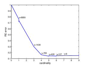
Figure 3: Example 2. Pareto trade-off curve.

In order to verify the reliability of an identified model, we carried out a leave-one-out (LOO) cross validation, on a subset of the available data. In particular, we used for cross validation data points $w(j)$ that lie within $0.75\%$ from the boundary of the the hyperrectangle defining the minimum and maximum deviation for each parameter (as defined in Table 1). This was done to avoid points near the boundary of the $w$ domain, which are too close to the non-explored region.

For each pair $(y(j),w(j))$ in the LOO validation set, a posynomial model has been identified from the data set $\mathfrak{D}\setminus(y(j),w(j))$. This model has then been tested on the single datum $(y(j),w(j))$, and the relative error $\nu_{j}=|y(j)-\hat{y}(j)|/\|y_{LOO}\|_{2}$ has been evaluated, where $\hat{y}(j)$ is the output provided by the model, and $\|y_{LOO}\|_{2}$ is the Euclidean norm of the vector with entries $y(j)$, for $j$ in the validation set. The accumulated relative error is given by $AE=\sqrt{\sum_{j}\nu_{j}^{2}}$. In our experiment, with $\gamma=785$, we obtained $AE=0.25$. This value appears to be quite low: a model identified using the proposed approach is able to approximate the unknown function quite accurately, even if only $50$ points are used to explore its 4-dimensional domain.

The same LOO validation has been performed considering $\gamma=1438$ and $\gamma=127$, obtaining $AE=0.38$ and $AE=0.25$, respectively. The model identified using $\gamma=785$ has thus the most advantageous trade-off between complexity and accuracy. This model is given by

$$\psi(w)=x_{340}\eta v^{2}+x_{440}\rho v^{2}+x_{465}\rho\eta v^{2}+x_{565}\rho^{2}v^{2}$$

where $x_{340}=1.2746\times 10^{-4}$, $x_{440}=3.5469\times 10^{-3}$, $x_{465}=2.8703\times 10^{-4}$, and $x_{565}=5.0722\times 10^{-4}$ (the units of these coefficient can be inferred from Table 1). It is interesting to note that a dependence of the drag force on the square velocity has been found by the algorithm and this result is consistent with the well-known drag equation. No significant dependence on the incidence angle $\theta$ has been observed. A possible interpretation for this latter result is that the range considered for $\theta$ is not sufficiently large compared to the ranges considered for $\rho$, $\eta$ and $v$ (see Table 1) and, consequently, the force variations due to $\theta$ are negligible with respect to those produced by the other three parameters.

We next discuss a few relevant aspects related to the identification process.

The safe feature elimination discussed in Section 3.3, reduced the number of columns of $\Phi$ from $625$ to $222$ (this latter is the average value obtained in the LOO validation), suggesting that this elimination phase can be quite useful in practical large-scale problems.

The time taken for applying the safe elimination and solving the optimization problem (8) with the approach described in Sections 3-5 is about $0.35$ seconds on a PC with a Core i7 processor and a RAM memory of 8GB (average time obtained in the LOO validation).

Acknowledgments: We thank Valentina Dolci (Politecnico di Torino) for providing us with the fluid dynamic simulation data used in the example.

7 Conclusions

An approach for the identification of posynomial models has been presented in this paper, based on the solution of a nonnegative regularized square-root LASSO problem. In this approach, a large-scale expansion of monomials is considered and the model is identified by seeking coefficients of the expansion that minimize an objective composed by a fitting error term and a sparsity promoting term. A sequential coordinate-descent scheme has been proposed to solve the nnrsqrt-LASSO problem. This scheme guarantees convergence to a minimum of the objective function and is suitable for large-scale implementations. Two numerical examples have finally been shown to demonstrate the effectiveness of the approach. The first one regards identification of a posynomial with negative and non integer exponents; the second one is about identification of a posynomial model for a NACA 4412 airfoil.

References

- [1] A. Babakhani, J. Lavaei, J. Doyle, and A. Hajimiri. Finding globally optimum solutions in antenna optimization problems. In IEEE International Symposium on Antennas and Propagation, 2010.
- [2] C.S. Beightler and D.T. Phillips. Applied geometric programming. Wiley, New York, 1976.
- [3] M. Bonin, V. Seghezza, and L. Piroddi. NARX model selection based on simulation error minimisation and LASSO. IET Control Theory and Applications, 4(7):1157–1168, 2010.
- [4] J.M. Boone, T.R. Fewell, and R.J. Jennings. Molybdenum, rhodium, and tungsten anode spectral models using interpolating polynomials with application to mammography. Medical Physics, 24(12):1863–1873, 1997.
- [5] S.P. Boyd, S.J. Kim, D.D. Patil, and M.A. Horowitz. Digital circuit optimization via geometric programming. Operation Research, 53(6):899–932, 2005.
- [6] E.J. Candes and T. Tao. Near-optimal signal recovery from random projections: Universal encoding strategies? IEEE Transactions on Information Theory, 52(12):5406 –5425, dec. 2006.
- [7] M. Chiang. Geometric programming for communication systems. Commun. Inf. Theory, 2:1–154, 2005.
- [8] W. Daems, G. Gielen, and W. Sansen. Simulation-based generation of posynomial performance models for the sizing of analog integrated circuits. IEEE Transactions on Computer-Aided Design of Integrated Circuits and Systems, 22(5):517–534, 2003.
- [9] D.L. Donoho, M. Elad, and V.N. Temlyakov. Stable recovery of sparse overcomplete representations in the presence of noise. IEEE Transactions on Information Theory, 52(1):6 – 18, jan. 2006.
- [10] R.J. Duffin, E.L. Peterson, and C. Zener. Geometric programming: theory and application. Wiley, New York, 1967.
- [11] L. El Ghaoui, V. Viallon, and T. Rabbani. Safe feature elimination for the LASSO and sparse supervised learning problems. Pacific Journal of Optimization, 8(4):667–698, 2012.
- [12] J. Fan and I. Gijbels. Local Polynomial Modelling and its Applications. Chapman & Hall, 1996.
- [13] J.J. Fuchs. Recovery of exact sparse representations in the presence of bounded noise. IEEE Transactions on Information Theory, 51(10):3601 –3608, oct. 2005.
- [14] W. Hoburg and P. Abbeel. Geometric programming for aircraft design optimization. In 8th AIAA MDO Specialist Conference, Honolulu, HI, USA, 2012.
- [15] H. Komiya. Elementary proof of sion’s minimax theorem. Kodai Math. J., 11:5–7, 1988.
- [16] S.L. Kukreja, J. Lofberg, and M.J. Brenner. A least absolute shrinkage and selection operator (LASSO) for nonlinear system identification. In 14th IFAC Symp. on System Identification, pages 814–819, Newcastle, Australia, 2006.
- [17] I. Lebert, V. Robles-Olvera, and A. Lebert. Application of polynomial models to predict growth of mixed cultures of pseudomonas spp. and listeria in meat. International Journal of Food Microbiology, 61(1):27–39, 2000.
- [18] I.J. Leontaritis and S.A. Billings. Input-output parametric models for non-linear systems - part i: deterministic non-linear systems. Int. J. Control, 41:303–328, 1985.
- [19] I.J. Leontaritis and S.A. Billings. Input-output parametric models for non-linear systems - part ii: stochastic non-linear systems. Int. J. Control, 41:329–344, 1985.
- [20] C. Liu. Gabor-based kernel pca with fractional power polynomial models for face recognition. IEEE Transactions on Pattern Analysis and Machine Intelligence, 26(5):572–581, 2004.
- [21] M. Milanese and C. Novara. Set membership identification of nonlinear systems. Automatica, 40/6:957–975, 2004.
- [22] C. Novara. Sparse identification of nonlinear functions and parametric set membership optimality analysis. IEEE Transactions on Automatic Control, 57(12):3236–3241, 2012.
- [23] C. Novara, L. Fagiano, and M. Milanese. Direct feedback control design for nonlinear systems. Automatica, 49(4):849–860, 2013.
- [24] T. Pulecchi and L. Piroddi. A cluster selection approach to polynomial NARX identification. In American Control Conference, pages 852–857, New York City, USA, 2007.
- [25] L. Quanhong and F. Caili. Application of response surface methodology for extraction optimization of germinant pumpkin seeds protein. Food Chemistry, 92(4):701–706, 2005.
- [26] S.S. Sapatnekar, V.B. Rao, P.M. Vaidya, and S.M. Kang. An exact solution to the transistor sizing problem for CMOS circuits using convex optimization. IEEE Transactions on Computer-Aided Design of Integrated Circuits and Systems, 12(11):1621–1634, 1993.
- [27] J.I. Schmidt, S. Evans, and J. Brinkmann. Comparison of polynomial models for land surface curvature calculation. International Journal of Geographical Information Science, 17(8):797–814, 2003.
- [28] M. Sion. On general minimax theorems. Pacific J. Math., 8:171–176, 1958.
- [29] W. Spinelli, L. Piroddi, and M. Lovera. A two-stage algorithm for structure identfication of polynomial NARX models. In American Control Conference, pages 2387–2392, 2006.
- [30] R Tibshirani. Regression shrinkage and selection via the Lasso. Royal. Statist. Soc B., 58(1):267–288, 1996.
- [31] J.A. Tropp. Just relax: convex programming methods for identifying sparse signals in noise. IEEE Transactions on Information Theory, 52(3):1030 –1051, mar. 2006.
- [32] P. Tseng. Convergence of a block coordinate descent method for nondifferentiable minimization. J. of Optimization Theory and Applications, 109(3):475–494, 2001.
- [33] D. Wilde. Globally optimal design. Wiley interscience publication, 1978.