Scaling of the Thue–Morse diffraction measure

Abstract

We revisit the well-known and much studied Riesz product representation of the Thue–Morse diffraction measure, which is also the maximal spectral measure for the corresponding dynamical spectrum in the complement of the pure point part. The known scaling relations are summarised, and some new findings are explained.

I Introduction

The Thue–Morse (TM) sequence is defined via the binary substitution $1\mapsto 1\bar{1}$, $\bar{1}\mapsto\bar{1}1$; see AS ; tao and references therein for general background. The corresponding dynamical system is known to have mixed (pure point and singular continuous) spectrum Q ; ME ; Kea , with a pure point part on the dyadic points and a singular continuous spectral measure in the form of a Riesz product. The latter coincides with the diffraction measure $\widehat{\gamma}$ of the TM Dirac comb with weights $\pm 1$; compare BG08 for details.

The Riesz product representation of the TM diffraction measure reads

$$\widehat{\gamma}\,=\prod_{n\geq 0}\bigl{(}1-\cos(2^{n+1}\pi k)\bigr{)},$$ (1)

with convergence (as a measure, not as a function) in the vague topology; see Z for general background. The singular continuous nature of $\widehat{\gamma}$ is traditionally proved Q ; Nat via excluding pure points by Wiener’s criterion Wie ; Mah and absolutely continuous parts by the Riemann–Lebesgue lemma Kaku ; compare BG08 ; tao and references therein for further material.

Since diffraction measures with singular continuous components do occur in practice Withers , it is of interest to study such measures in more detail. Below, we use the TM paradigm to rigorously explore the scaling properties of ‘singular peaks’ in a diffraction measure, combining methods from harmonic analysis and number theory; for further results of a similar type, we refer to CSM ; GL ; Zaks ; ZPK1 ; ZPK2 and references therein.

II Ergodicity properties

In what follows, we employ various Birkhoff sums, and implicitly explore a range of uniform distribution properties, either on the unit interval $[0,1]$ or on various finite subsets of it; we refer to KN for background.

Let us first observe that the mapping $T$ defined by $x\mapsto 2\hskip 0.5ptx\bmod 1$ maps $[0,1]$ into itself and leaves Lebesgue measure invariant. Moreover, $T$ is ergodic relative to Lebesgue measure HL ; Kac , wherefore Birkhoff’s ergodic theorem gives us the following result.

Lemma 1

Let $g\in L^{1}\bigl{(}[0,1]\bigr{)}$ and consider the mapping $T$ defined by $x\mapsto 2\hskip 0.5ptx\bmod 1$. Then, for Lebesgue almost every point $k\in[0,1]$, one has

$$\lim_{N\to\infty}\frac{1}{N}\sum_{n=0}^{N-1}g(T^{n}(k))\,=\int_{0}^{1}g(x)\,\mathrm{d}x\hskip 0.5pt.$$

Consider the function $f$ defined by

$$f(x)\,=\,\log\bigl{(}1-\cos(2\pi x)\bigr{)}$$

on $[0,1]$. It has singularities at $x=0$ and $x=1$, which are both integrable (via standard arguments), so $f\in L^{1}\bigl{(}[0,1]\bigr{)}$. Note that $f$ is not Riemann integrable in the proper sense, though it is in the generalised sense of an improper integral. Still, this means that we cannot directly apply uniform distribution without some additional argument, which is ultimately equivalent to the approach via Birkhoff sums. In fact, since $f$ has an obvious extension to a $1$-periodic function on $\mathbb{R}\hskip 0.5pt$, sums of the form $\frac{1}{N}\sum_{n=0}^{N-1}f(2^{n+1}\pi x)$ can be analysed, for almost all $x\in\mathbb{R}\hskip 0.5pt$, via Lemma 1.

Here, via an explicit calculation, one gets

$$\int_{0}^{1}\log\bigl{(}1-\cos(2\pi x)\bigr{)}\,\mathrm{d}x\,=\,-\log(2)\,.$$ (2)

We shall also need a discrete analogue of this formula. Via $1-\cos(2\vartheta)=2\bigl{(}\sin(\vartheta)\bigr{)}^{2}$ together with the well-known identity $\prod_{m=1}^{n-1}\sin(\pi\frac{m}{n})=n/2^{n-1}$, one can derive that

$$\sum_{m=1}^{n-1}\log\bigl{(}1-\cos(2\pi\tfrac{m}{n})\bigr{)}\,=\,\log\biggl{(}\frac{n^{2}}{2_{\phantom{T}}^{n-1}}\biggr{)}$$ (3)

holds for all $n\geq 1$, with obvious meaning for $n=1$.

III Riesz product

A direct path to the Riesz product of the TM diffraction measure can be obtained as follows. Consider the recursion $v^{(n+1)}=v^{(n)}\bar{v}^{(n)}$ with initial condition $v^{(0)}=1$, which gives an iteration towards the one-sided fixed point $v$ of the TM substitution on the alphabet $\{1,\bar{1}\}$. If we define the exponential sum

$$g_{n}(k)\,=\,\sum_{\ell=0}^{2^{n}-1}v_{\ell}\,e^{-2\pi ik\ell},$$

where $v=v_{0}v_{1}v_{2}\cdots$, the function $g_{n}$ is then the Fourier transform of the weighted Dirac comb for $v_{n}$, when it is realised with Dirac measures (of weight $\pm 1$) on the left endpoints of the unit intervals that represent the symbolic sequence of $v_{n}$. In particular, one has $g_{0}(k)=1$ and

$$g_{n+1}(k)\,=\,\bigl{(}1-e^{-2\pi ik2^{n}}\bigr{)}\,g_{n}(k)$$

for $n\geq 0$, so that

$$\bigl{|}g_{n+1}(k)\bigr{|}^{2}\,=\,2\hskip 0.5pt\bigl{|}g_{n}(k)\bigr{|}^{2}\bigl{(}1-\cos(2^{n+1}\pi k)\bigr{)}.$$

One can then explicitly check that

$$f_{n}(k)\,:=\,\frac{1}{2^{n}}\bigl{|}g_{n}(k)\bigr{|}^{2}=\prod_{\ell=0}^{n-1}\bigl{(}1-\cos(2^{\ell+1}\pi k)\bigr{)}\hskip 0.5pt,$$

which reproduces the Riesz product of Eq. (1) in the sense that $\lim_{n\to\infty}f_{n}=\widehat{\gamma}$ as measures in the vague topology.

As $g_{n}$ corresponds to a chain of length $2^{n}$, the growth rate $\beta(k)$ of the intensity at $k$ (when this rate is well-defined) is obtained as

$$\beta(k)\,=\,\lim_{n\to\infty}\frac{\log\bigl{(}f_{n}(k)\bigr{)}}{n\hskip 0.5pt\log(2)}\hskip 0.5pt.$$

Let us now consider the growth rate for various cases of the wave number $k$.

Case A. When $k=\frac{m}{2^{r}}$ with $r\geq 0$ and $m\in\mathbb{Z}$, all but finitely many factors of the Riesz product (1) vanish, so that no contribution can emerge from such values of $k$. In fact, these are the dyadic points, which support the pure point part of the dynamical spectrum. They are extinction points for the diffraction measure of the balanced weight case considered here; compare ME for a discussion of this connection.

Case B. Since $f$ is a $1$-periodic function, we clearly have $\beta(k)=\beta(k\bmod 1)$, so we can use Birkhoff sums with arguments reduced to the unit interval in conjunction with Lemma 1. Then, for Lebesgue almost all $k\in\mathbb{R}\hskip 0.5pt$, one obtains the growth rate

$$\beta(k) =\lim_{N\to\infty}\frac{1}{N}\sum_{n=0}^{N-1}\frac{\log\bigl{(}1-\cos(2^{n+1}\pi k)\bigr{)}}{\log(2)}$$

$$=\int_{0}^{1}\frac{\log\bigl{(}1-\cos(2\pi x)\bigr{)}}{\log(2)}\,\mathrm{d}x\,=-1\hskip 0.5pt.$$

Such wave numbers $k$ thus do not contribute to the TM measure.

Among the values $k$ for which this is true, we have (possibly up to a null set) those ones for which the sequence $\bigl{(}2^{n}k\bigr{)}_{n\in\mathbb{N}_{0}}$ is uniformly distributed modulo $1$, none of which ever visits a dyadic point, and thus never meets the singular points of $f$.

Note that this argument shows that $\lim_{n\to\infty}f_{n}(k)=0$ pointwise for almost all $k\in\mathbb{R}\hskip 0.5pt$ and thus provides an alternative proof of the fact that the measure from Eq. (1) does not comprise an absolutely continuous part; compare the Introduction as well as Kaku ; BG08 .

Case C. When $k=\frac{m}{3}$ with $m$ not divisible by $3$, one finds $f_{n}(k)=(3/2)^{n}$. Since this corresponds to a system (or sequence) of length $2^{n}$, we have a growth rate of

$$\beta(k)\,=\,\frac{\log(3/2)}{\log(2)}\,\approx\,0.584963\,.$$

The same growth rate applies to all numbers of the form $k=\frac{m}{2_{\vphantom{I}}^{r}\cdot\,3}$ with $r\geq 0$ and $m$ not divisible by $3$, because the factor $2^{r}$ in the denominator has no influence on the asymptotic scaling, due to the structure of the Riesz product (1). Note that the points of this form are dense in $\mathbb{R}\hskip 0.5pt$, but countable.

Similarly, when $k=\frac{m}{2_{\vphantom{I}}^{r}\cdot\,5}$ with $r\geq 0$ and $m$ not a multiple of $5$, one finds

$$\beta(k)\,=\,\frac{\log(5/4)}{2\hskip 0.5pt\log(2)}\,\approx\,0.160964\,.$$

Case D. More generally, when ${k=\frac{p}{2_{\vphantom{I}}^{r}q}}$ with ${r\geq 0}$, ${q\geq 3}$ odd and $\gcd(p,q)=1$, one can determine the growth rate explicitly. Recall that ${U_{q}}:={(\mathbb{Z}/q\mathbb{Z})^{\times}}={\{1\leq p<q\mid\gcd(p,q)=1\}}$ is the unit group of the finite residue class ring $\mathbb{Z}/q\mathbb{Z}$. If $S_{q}={\{2^{n}\bmod q\mid n\geq 0\}}$ is the subgroup of $U_{q}$ generated by the unit $2$, one finds

$$\beta(k)\,=\,\frac{1}{\mathrm{card}(p\hskip 0.5ptS_{q})}\sum_{n\in pS_{q}}\frac{\log\bigl{(}1-\cos(2\pi\frac{n}{q})\bigr{)}}{\log(2)}$$ (4)

by an elementary calculation. When $q=2m+1$, the integer $\mathrm{card}(S_{q})$ is the multiplicative order of $2$ mod $q$, which is sequence A 002326 in Sloane .

When $\gcd(p,q)=1$, one has $\mathrm{card}(p\hskip 0.5ptS_{q})=\mathrm{card}(S_{q})$, even when the set $p\hskip 0.5ptS_{q}$ is considered mod $q$. Note that formula (4) is written in such a way that it also holds for all $p$ not divisible by $q$. If $\gcd(p,q)>1$, the set $p\hskip 0.5ptS_{q}$ may be reduced mod $q$, which shows that the formula consistently gives $\beta(p/q)$ in such cases.

Case E. When $\mathrm{card}(S_{q})=q-1$, Eq. (3) leads to $\beta(1/q)=g(q)$ with

$$g(q)\,=\,\frac{\log\Bigl{(}\frac{q^{2}}{2_{\vphantom{I}}^{q-1}}\Bigr{)}}{\log\bigl{(}2_{\vphantom{I}}^{q-1}\bigr{)}}\,=\,\frac{2\hskip 0.5pt\log(q)}{(q-1)\log(2)}-1\hskip 0.5pt.$$ (5)

For odd $q\geq 3$, the function $g(q)$ is positive precisely for $q=3$ and $q=5$, and negative otherwise; compare Figure 1. In fact, also $\beta(1/q)$ seems to be negative for all odd $q\geq 7$, though this does not hold for general $\beta(p/q)$. Indeed, $\beta(3/17)>0$, and all positive exponents for odd $7\leq q<1000$ are listed in Table 1.

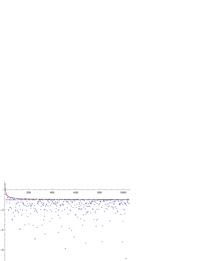
Figure 1: Exponents $\beta(1/q)$ according to Eq. (4) for all odd $3\leq q<1050$. Apart from $q=3$ and $q=5$, the exponents are negative. The solid line is the function $g$ from Eq. (5). Exponents with large negative values emerge for $q=2^{r}\pm 1$.

More generally, for any odd $q\geq 3$, one obtains (from Case D) the formula

$$\frac{1}{q-1}\sum_{1<d|q}\mathrm{card}(S_{d})\sum_{p\in U_{d}/S_{d}}\beta\bigl{(}\tfrac{p}{d}\bigr{)}\,=\,g(q)\hskip 0.5pt.$$ (6)

Now, Möbius inversion (with the Möbius function $\mu$) leads to

$$\sum_{p\in U_{q}/S_{q}}\beta\bigl{(}\tfrac{p}{q}\bigr{)}\,=\,\frac{1}{\mathrm{card}(S_{q})}\sum_{1\neq d|q}\mu\bigl{(}\tfrac{q}{d}\bigr{)}\,(d-1)\,g(d)\hskip 0.5pt,$$ (7)

while it seems difficult to find a simpler formula than Eq. (4) for the individual exponents in general.

Case F. As is shown in CSM (by way of an explicit example), there are wave numbers $k$ for which the exponent $\beta(k)$ does not exist. The construction is based on a suitable mixture of binary expansions for wave numbers with different exponents. Clearly, there are uncountably many such examples, though they still form a null set. Here, one can define a ‘spectrum’ of exponents via the limits of all converging subsequences.

Table 1: Wave numbers $k=\frac{p}{q}$ with positive exponents, for all odd integers $5<q<1000$. For a given $q$, all $p\in U_{q}/S_{q}$ are considered (we choose the smallest element of the set $p\hskip 0.5ptS_{q}$ mod $q$ as representative).

$\frac{p}{q}$	$\,\beta\bigl{(}\frac{p}{q}\bigr{)}$	$\frac{p}{q}$	$\,\beta\bigl{(}\frac{p}{q}\bigr{)}$	$\frac{p}{q}$	$\,\beta\bigl{(}\frac{p}{q}\bigr{)}$	$\frac{p}{q}$	$\,\beta\bigl{(}\frac{p}{q}\bigr{)}$	$\frac{p}{q}$	$\,\beta\bigl{(}\frac{p}{q}\bigr{)}$	$\frac{p}{q}$	$\,\beta\bigl{(}\frac{p}{q}\bigr{)}$
$\frac{3}{17}$	0.266	$\frac{25}{117}$	0.172	$\frac{37}{255}$	0.150	$\frac{65}{381}$	0.067	$\frac{47}{565}$	0.144	$\frac{65}{771}$	0.140
$\frac{5}{31}$	0.272	$\frac{19}{127}$	0.108	$\frac{43}{255}$	0.318	$\frac{47}{451}$	0.127	$\frac{81}{565}$	0.113	$\frac{161}{771}$	0.140
$\frac{11}{31}$	0.272	$\frac{21}{127}$	0.373	$\frac{53}{255}$	0.318	$\frac{65}{451}$	0.127	$\frac{61}{585}$	0.126	$\frac{69}{775}$	0.101
$\frac{5}{33}$	0.105	$\frac{27}{127}$	0.108	$\frac{91}{255}$	0.150	$\frac{67}{455}$	0.128	$\frac{97}{585}$	0.126	$\frac{83}{775}$	0.127
$\frac{7}{43}$	0.267	$\frac{43}{127}$	0.373	$\frac{37}{257}$	0.049	$\frac{69}{455}$	0.128	$\frac{53}{595}$	0.031	$\frac{111}{775}$	0.127
$\frac{11}{63}$	0.244	$\frac{19}{129}$	0.143	$\frac{43}{257}$	0.404	$\frac{53}{511}$	0.028	$\frac{87}{595}$	0.031	$\frac{117}{775}$	0.101
$\frac{13}{63}$	0.244	$\frac{11}{151}$	0.012	$\frac{45}{257}$	0.221	$\frac{75}{511}$	0.163	$\frac{51}{601}$	0.042	$\frac{57}{785}$	0.085
$\frac{11}{65}$	0.350	$\frac{35}{151}$	0.012	$\frac{23}{275}$	0.117	$\frac{83}{511}$	0.239	$\frac{63}{601}$	0.042	$\frac{137}{819}$	0.359
$\frac{11}{73}$	0.165	$\frac{25}{171}$	0.220	$\frac{49}{275}$	0.117	$\frac{85}{511}$	0.422	$\frac{53}{657}$	0.061	$\frac{145}{819}$	0.359
$\frac{13}{73}$	0.165	$\frac{19}{185}$	0.126	$\frac{25}{331}$	0.067	$\frac{87}{511}$	0.028	$\frac{101}{657}$	0.061	$\frac{67}{825}$	0.089
$\frac{13}{89}$	0.229	$\frac{17}{195}$	0.001	$\frac{35}{337}$	0.149	$\frac{107}{511}$	0.239	$\frac{51}{673}$	0.038	$\frac{173}{825}$	0.089
$\frac{19}{89}$	0.229	$\frac{41}{195}$	0.001	$\frac{57}{337}$	0.149	$\frac{109}{511}$	0.163	$\frac{57}{683}$	0.131	$\frac{67}{889}$	0.050
$\frac{9}{91}$	0.075	$\frac{17}{205}$	0.047	$\frac{49}{341}$	0.060	$\frac{171}{511}$	0.422	$\frac{71}{683}$	0.087	$\frac{95}{889}$	0.012
$\frac{19}{91}$	0.075	$\frac{31}{205}$	0.183	$\frac{57}{341}$	0.369	$\frac{43}{513}$	0.033	$\frac{103}{683}$	0.179	$\frac{129}{889}$	0.012
$\frac{11}{105}$	0.060	$\frac{19}{217}$	0.073	$\frac{71}{341}$	0.369	$\frac{77}{513}$	0.122	$\frac{111}{683}$	0.226	$\frac{157}{889}$	0.050
$\frac{17}{105}$	0.060	$\frac{37}{217}$	0.073	$\frac{73}{341}$	0.060	$\frac{83}{513}$	0.272	$\frac{113}{683}$	0.335	$\frac{83}{993}$	0.124
$\frac{17}{117}$	0.172	$\frac{35}{241}$	0.194	$\frac{31}{381}$	0.067	$\frac{85}{513}$	0.343	$\frac{55}{753}$	0.054	$\frac{149}{993}$	0.172

Case G. So far, we have identified countably many values of $k$, for which the scaling exponents can be calculated, while (due to Case B) Lebesgue-almost all $k\in\mathbb{R}\hskip 0.5pt$ carry no singular peak. The remaining problem is to cope with the uncountably many wave numbers (of zero Lebesgue measure) that belong to the supporting set of the TM measure and may possess well-defined exponents.

The existence of such numbers can be understood via Diophantine approximation. Again, it is useful to start with the binary expansion of a wave number $k$, and then modify it in a suitable way. Consider first the example

$$k\,=\,\tfrac{1}{3}\,=\,0.0101010101\ldots$$

If we now switch the binary digits at positions $2^{r}$, with $r\in\mathbb{N}$, we obtain a different wave number $k^{\prime}$ that is irrational but nevertheless still has the same scaling exponent $\beta$ as $k=\frac{1}{3}$, as longer and longer stretches of the binary expansion of $k^{\prime}$ agree with that of $k$. Clearly, via similar modifications, we can obtain uncountably many distinct irrational numbers with $\beta=\beta(1/3)$.

The same strategy works for all other rational wave numbers $k$, and underlies the nature of the TM measure. In particular, this explains the existence of uncountably many ‘singular peaks’, which together (in view of Case B) still form a Lebesgue null set. These scaling exponents are accessible via our above arguments. It would be interesting to see whether one can go any further with the pointwise analysis.

To continue, it would be natural to augment the above results by a proper analysis of the full TM measure, along the lines of GL ; Wolny ; Zaks ; ZPK1 ; ZPK2 and related works. Also, a better understanding of the set of wave numbers for which the exponent $\beta(k)$ is well-defined would be welcome.

IV Concluding remarks

An analogous approach works for all measures of the form of a classic Riesz product. In particular, the generalised Thue–Morse sequences from BGG can be analysed along these lines; compare also Kea . Likewise, the choice of different interval lengths is possible, though technically more complicated; compare Wolny for some examples.

Higher-dimensional examples with purely singular continuous spectrum, such as the squiral tiling squiral or similar bijective block substitutions Nat , may still lead to classic Riesz products, though they are now in more than one variable, and the analysis is hence more involved. Nevertheless, the scaling analysis will still lead to a better understanding of such measures.

References

- (1) J.-P. Allouche and J. Shallit, Automatic Sequences: Theory, Applications, Generalizations, Cambridge University Press, Cambridge (2003).
- (2) M. Baake and U. Grimm, The singular continuous diffraction measure of the Thue–Morse chain, J. Phys. A: Math. Theor. 41, 422001 (2008); arXiv:0809.0580.
- (3) M. Baake and U. Grimm, Squirals and beyond: Substitution tilings with singular continuous spectrum, Erg. Th. & Dynam. Syst., in press; arXiv:1205.1384.
- (4) M. Baake and U. Grimm, Aperiodic Order. Vol. : A Mathematical Invitation, Cambridge University Press, Cambridge (2013).
- (5) M. Baake, F. Gähler and U. Grimm, Spectral and topological properties of a family of generalised Thue–Morse sequences, J. Math. Phys. 53, 032701 (2012); arXiv:1201.1423.
- (6) Z. Cheng, R. Savit and R. Merlin, Structure and electronic properties of Thue–Morse lattices, Phys. Rev. B 37, 4375–4382 (1988).
- (7) N.P. Frank, Multi-dimensional constant-length substitution sequences, Topol. Appl. 152, 44–69 (2005).
- (8) C. Godréche and J.M. Luck, Multifractal analysis in reciprocal space and the nature of the Fourier transform of self-similar structures, J. Phys. A: Math. Gen. 23, 3769–3797 (1990).
- (9) G.H. Hardy and J.E. Littlewood, Some problems of Diophantine approximation, Acta Math. 37, 155–191 (1914).
- (10) M. Kac, On the distribution of values of sums of the type , Ann. Math. 47, 33–49 (1946).
- (11) S. Kakutani, Strictly ergodic symbolic dynamical systems, in: Proc. 6th Berkeley Symposium on Math. Statistics and Probability eds L.M. LeCam, J. Neyman and E.L. Scott, Univ. of California Press, Berkeley (1972), pp. 319–326.
- (12) M. Keane, Generalized Morse sequences, Z. Wahrscheinlichkeitsth. verw. Geb. 10, 335–353 (1968).
- (13) L. Kuipers and H. Niederreiter, Uniform Distribution of Sequences, Wiley, New York (1974); reprint Dover, New York (2006).
- (14) K. Mahler, The spectrum of an array and its application to the study of the translation properties of a simple class of arithmetical functions. Part II: On the translation properties of a simple class of arithmetical functions, J. Math. Massachusetts 6, 158–163 (1927).
- (15) M. Queffélec, Substitution Dynamical Systems – Spectral Analysis, LNM 1294, 2nd ed., Springer, Berlin (2010).
- (16) N.J.A.S. Sloane, The On-Line Encyclopedia of Integer Sequences, available at http://oeis.org/.
- (17) A.C.D. van Enter and J. Miȩkisz, How should one define a weak crystal? J. Stat. Phys. 66, 1147–1153 (1992).
- (18) N. Wiener, The spectrum of an array and its application to the study of the translation properties of a simple class of arithmetical functions. Part I: The spectrum of an array, J. Math. Massachusetts 6, 145–157 (1927).
- (19) R.L. Withers, Disorder, structured diffuse scattering and the transmission electron microscope, Z. Krist. 220, 1027–1034 (2005).
- (20) J. Wolny, A. Wnȩk and J.-L. Verger-Gaugry, Fractal behaviour of diffraction pattern of Thue–Morse sequence J. Comput. Phys. 163, 313–327 (2000).
- (21) M.A. Zaks, On the dimensions of the spectral measure of symmetric binary substitutions, J. Phys. A: Math. Gen. 35, 5833–5841 (2002).
- (22) M.A. Zaks, A.S. Pikovsky and J. Kurths, On the correlation dimension of the spectral measure for the Thue–Morse sequence, J. Stat. Phys. 88, 1387–1392 (1997).
- (23) M.A. Zaks, A.S. Pikovsky and J. Kurths, On the generalized dimensions for the Fourier spectrum of the Thue–Morse sequence, J. Phys. A: Math. Gen. 32, 1523–1530 (1999).
- (24) A. Zygmund, Trigonometric Series, 3rd ed., Cambridge University Press, Cambridge (2002).