A new approach to time-dependent transport through an interacting quantum dot within Keldysh formalism

Abstract

The time-dependent transport through a nano-scale device, consisting of a single spin-degenerate orbital with on-site Coulomb interaction, coupled to two leads, is investigated. Various gate and bias voltage time-dependences are considered. The key and new point lies in the proposed way to avoid the difficulties of the usual heavy computation when dealing with two time Green’s functions within Keldysh formalism. The time-dependent retarded dot Green’s functions are evaluated, in an efficient manner within a non-canonical Hubbard I approximation. Calculations of the time-dependent current are then presented in the wide-band limit for different parameter sets. A comparison between the method and the Hartree-Fock approximation is performed as well. It is shown that the later cannot account reliably for dynamical aspects of transport phenomena.

I Introduction

The investigation of electron transport in nano-structures, such as quantum dots or carbon nanotubes, is of high actual interest. It leads to the observation of a multitude of mesoscopic phenomena, where the dual nature of quasi-particles is readily observed. Its wave character is manifest in interference phenomena due to the phase coherence of charge carriers, whereas its granular character is best visible in the Coulomb blockade effect Altshuler91 ; DattaBook ; HaugJauhoBook . Besides their fundamental character, mesoscopic transport studies are also of high technological interest. It is sufficient to quote the development of carbon nanotube transistors Appenzeller04 , which can operate up to terahertz frequencies Zhong08 .

Several complications arise for the theoretical description of transport properties in nanodevices which are beyond solid state physics outlined in classical text-books. These include nonadiabatic effects and time dependent phenomena, as well as the wealth of properties induced by Coulomb correlations. For a realistic description, all these effects have to be treated simultaneously. This is a real challenge. Nonadiabatic time dependent effects are usually treated within the framework of two-time Keldysh Green’s functions JauhoWingreenMeir1994 , but the treatment of the Coulomb interaction is indispensable in most cases. One can distinguish three levels of correlation effects: (i) weak Coulomb correlation of either Hartree (electrostatic interaction) or Hartree-Fock (including spin exchange) character, (ii) Coulomb blockade, and (iii) Kondo physics. The two crucial parameters that guide Coulomb effects are the coupling between dot and electrodes, and the temperature. By decreasing these two parameters the Coulomb effects become more and more important, the Kondo physics taking place at low temperature, for a low bias voltage. To simulate the terahertz response of carbon nanotube transistors, the treatment of weak correlation effects (in Hartree approximation) is already a standard procedure Kienle09 . However, a well developed time-dependent formalism in case of strong correlation and a fortiori when Coulomb-induced collective phenomena set in, deserves to be improved, and is currently a very active research area.

Here, we present a formalism of non-adiabatic electron transport which is able to treat an arbitrary time-dependence of bias and gate voltages, as well as a time-dependence of the hybridization between leads and dot. The transient and steady-state properties can be evaluated, without any a priory assumption about adiabatic or sudden limits. Our formalism includes the effects of Coulomb correlations beyond weak-coupling treatment, and works for arbitrary on-site interaction $U$. Our approach is not restricted to the wide-band limit, although the presented numerical results rely on it. It treats correctly the uncorrelated ($U\to 0$) and the atomic (disconnected dot) limits, but cannot account for the Kondo effect, albeit interplay between transient phenomena and Kondo physics are very interesting issues Nordlander99 , PlihalLangreth2000 . As a consequence the temperatures considered here are higher than the Kondo temperature $T_{K}$.

The formalism is based on a systematic use of two-time Keldysh Green’s functions in the Hubbard I approximation (HIA) Hubbard1963 ; Hewson66 . The key and new point lies in the proposed way to circumvent the difficulties of the usual heavy computation when dealing with two time Green’s functions. Our approach is easy to implement and constitutes a substantial computer-time saving method. This advantage is shared with the technique recently developed by Croy and Saalman CroySaalmann85 . The approaches are different in detail but predict consistent results, as shown later.

After having presented the general formalism in Sec. 2, we show in some detail the main idea of our approximation in Sec. 3. First we apply the approach to a steady-state case (Sec.4). This allows us to compare our correlation treatment to the Hartree-Fock (HF) approximation, and also to a more sophisticated correlation treatment, namely the noncrossing approximation (NCA) Bickers . For the parameters under study, the NCA with a renormalized Hubbard bandwidth and HIA in the non-equilibrium steady-state regime compare favorably, while HF turns to be unreliable myohaetal . In the time-dependent situation (Sec. 5) we investigate the case of a pulse modulation for the bias voltage, which enables to measure the charging time in the Coulomb blockade regime, as well as the tunnel and displacement currents. We then investigate the case of a forced harmonic bias voltage, with transient and steady-state regimes, before turning to the case of a pure pumping experiment, where, along the lines developed by Croy et al. CroySaalmann85 , we address the question of adiabatic Splettstoesser05 and non-adiabatic frontier. We finally close with our Conclusions (Sec. 6).

II Model Hamiltonian and general expression for time-dependent current

We consider a system which is a single level interacting Anderson quantum dot, coupled to two uncorrelated leads, acting as source and drain. The Hamiltonian reads Anderson

$$H=H_{c}+H_{T}+H_{\rm cen}.$$ (1)

$H_{c}$ is a contact Hamiltonian corresponding to electrons in leads, and takes the following form

$$H_{c}=\sum_{k\alpha\sigma}\varepsilon_{k\alpha}(t)\mathbf{c}_{k\alpha\sigma}^{\dagger}\mathbf{c}_{k\alpha\sigma},$$ (2)

where $k$ denotes momentum index, $\alpha=(L,R)$ stands for left and right leads and $\sigma=(\uparrow,\downarrow)$ is the spin degree of freedom. Here $\mathbf{c}_{k\alpha\sigma}^{\dagger}$ and $\mathbf{c}_{k\alpha\sigma}$ are electron creation and annihilation operators for the $\alpha$-lead state $k\sigma$. $H_{T}$ is a coupling term

$$H_{T}=\sum_{k\alpha\sigma}\left[V_{k\alpha}(t)\mathbf{c}_{k\alpha\sigma}^{\dagger}\mathbf{d}_{\sigma}+V_{k\alpha}^{*}(t)\mathbf{d}_{\sigma}^{\dagger}\mathbf{c}_{k\alpha\sigma}\right],$$ (3)

where $\mathbf{d}_{\sigma}^{\dagger}$ and $\mathbf{d}_{\sigma}$ are electron creation and annihilation operators at the dot for spin state $\sigma$. The central region Hamiltonian $H_{\rm cen}$ includes Coulomb repulsion term:

$$H_{\rm cen}=\varepsilon_{0}(t)\sum_{\sigma}\mathbf{d}_{\sigma}^{\dagger}\mathbf{d}_{\sigma}+U\mathbf{d}_{\uparrow}^{\dagger}\mathbf{d}_{\uparrow}\mathbf{d}_{\downarrow}^{\dagger}\mathbf{d}_{\downarrow}.$$ (4)

The energy level in the dot $\varepsilon_{0}(t)$, in the leads $\varepsilon_{k\alpha}(t)=\varepsilon_{k}^{0}+\Delta_{\alpha}(t)$, as well as the hybridization coefficients $V_{k\alpha}(t)$, are all considered to be time dependent, and independent of each other. Experimentally, that can be realized by applying different bias and gate voltages. We shall use the assumption that the time dependence of the hybridization parameters can be factorized as $V_{k\alpha}(t)=u_{\alpha}(t)V_{\alpha}(\varepsilon^{0}_{k})$ JauhoWingreenMeir1994 .

Current from left contact to the central region can be calculated as

$$J_{L}(t)=-e\langle\dot{N_{L}}(t)\rangle=-i\frac{e}{\hbar}\langle[H,N_{L}]\rangle,$$ (5)

where $N_{L}$ is the lead fermion number operator. Similar problem was considered recently CroySaalmann85 in the wide-band limit with a density matrix approach using a truncated equation of motion technique. In the present paper we apply the time-dependent Keldysh formalism Keldysh . The expression for the current can be written in terms of central region Keldysh Green’s functions (see Ref. JauhoWingreenMeir1994 )

$$J_{L}(t) = -2\frac{e}{\hbar}\int_{-\infty}^{t}dt_{1}\int\frac{d\varepsilon}{2\pi}\mathrm{Im}\sum_{\sigma}\left\{\right.e^{-i\varepsilon(t_{1}-t)}\Gamma^{L}(\varepsilon,t_{1},t)$$ (6)

$$\times \left[G_{\sigma\sigma}^{<}(t,t_{1})+f_{L}(\varepsilon)G_{\sigma\sigma}^{r}(t,t_{1})\right]\left.\right\}.$$

Here $\Gamma^{L}(\varepsilon,t_{1},t)$ is defined as

$$\Gamma^{\alpha}(\varepsilon,t_{1},t) = 2\pi\rho(\varepsilon)u_{\alpha}(t)u_{\alpha}(t_{1})V_{\alpha}(\varepsilon)V_{\alpha}^{*}(\varepsilon)$$ (7)

$$\times\exp\left[i\int_{t_{1}}^{t}dt_{2}\Delta_{\alpha}(t_{2})\right],$$

where $\rho(\varepsilon)$ is the density of states per lead and per spin, which we choose independent of $\alpha$. $f_{L}(\varepsilon)$ is the Fermi distribution function of the left contact. Finally $G_{\sigma\sigma}^{<}(t,t_{1})$ and $G_{\sigma\sigma}^{r}(t,t_{1})$ are the lesser and retarded Keldysh Green’s functions of the central region

$$G_{\sigma\sigma}^{<}(t,t^{\prime}) = i\langle\mathbf{d}_{\sigma}^{\dagger}(t^{\prime})\mathbf{d}_{\sigma}(t)\rangle,$$ (8)

$$G_{\sigma\sigma}^{r}(t,t^{\prime}) = -i\operatorname{\theta}(t-t^{\prime})\langle\{\mathbf{d}_{\sigma}(t),\mathbf{d}_{\sigma}^{\dagger}(t^{\prime})\}\rangle.$$ (9)

Even out of equilibrium, the Green’s functions are diagonal in spin, due to our choice for $H$ which conserves spin. In order to calculate the time-dependent current one needs to calculate these Green’s functions first.

III Green’s functions of the central region

III.1 Equation of motion for Green’s functions

We calculate the equation of motion for the retarded Green’s function $G_{\sigma\sigma}^{r}(t,t^{\prime})$. It leads to

$$\left(i\frac{\partial}{\partial t}-\varepsilon_{0}(t)\right)G_{\sigma\sigma}^{r}(t,t^{\prime}) = \delta(t-t^{\prime})+\sum_{k\alpha}V^{*}_{k\alpha}(t)G_{k\alpha\sigma,\sigma}^{r}(t,t^{\prime})$$ (10)

$$+ UG_{\sigma\sigma,U}^{r}(t,t^{\prime}),$$

where two other Green’s functions appear: $G_{\sigma\sigma,U}^{r}(t,t^{\prime})=-i\operatorname{\theta}(t-t^{\prime})\langle\{(\mathbf{d}_{\sigma}\mathbf{d}_{\bar{\sigma}}^{{\dagger}}\mathbf{d}_{\bar{\sigma}})(t),\mathbf{d}_{\sigma}^{\dagger}(t^{\prime})\}\rangle$ and $G_{k\alpha\sigma,\sigma}^{r}(t,t^{\prime})=-i\operatorname{\theta}(t-t^{\prime})\langle\{\mathbf{c}_{k\alpha\sigma}(t),\mathbf{d}_{\sigma}^{\dagger}(t^{\prime})\}\rangle$. The equation of motion for $G_{k\alpha\sigma,\sigma}^{r}(t,t^{\prime})$ is

$$\left(i\frac{\partial}{\partial t}-\varepsilon_{k\alpha}(t)\right)G_{k\alpha\sigma,\sigma}^{r}(t,t^{\prime})=V_{k\alpha}(t)G_{\sigma\sigma}^{r}(t,t^{\prime}).$$ (11)

The formal solution of this equation can be written as

$$G_{k\alpha\sigma,\sigma}^{r}(t,t^{\prime})=\int dt_{1}g_{k\alpha}^{r}(t,t_{1})V_{k\alpha}(t_{1})G_{\sigma\sigma}^{r}(t_{1},t^{\prime}),$$ (12)

where $g_{k\alpha}^{r}(t,t_{1})$ is the Green’s function for the uncoupled system

$$g_{k\alpha}^{r}(t,t^{\prime})=-i\operatorname{\theta}(t-t^{\prime})\exp\left[-i\int_{t^{\prime}}^{t}dt_{1}\varepsilon_{k\alpha}(t_{1})\right].$$ (13)

Substituting (12) into the equation for $G_{\sigma\sigma}^{r}(t,t^{\prime})$ (10), we get

$$\left(i\frac{\partial}{\partial t}-\varepsilon_{0}(t)\right)G_{\sigma\sigma}^{r}(t,t^{\prime})=\delta(t-t^{\prime})$$

$$+\int dt_{1}\Sigma^{r}(t,t_{1})G_{\sigma\sigma}^{r}(t_{1},t^{\prime})+UG_{\sigma\sigma,U}^{r}(t,t^{\prime}),$$ (14)

where $\Sigma^{r}(t,t^{\prime})$ is the hybridization self-energy

$$\Sigma^{r}(t,t^{\prime}) = \sum_{k\alpha}V^{*}_{k\alpha}(t)g_{k\alpha}^{r}(t,t^{\prime})V_{k\alpha}(t^{\prime})$$

$$= -i\operatorname{\theta}(t-t^{\prime})\sum_{\alpha}\int\frac{d\varepsilon}{2\pi}e^{-i\varepsilon(t-t^{\prime})}\Gamma^{\alpha}(\varepsilon,t,t^{\prime}).$$

Equation (14) is not a closed equation for $G_{\sigma\sigma}^{r}(t,t^{\prime})$ because of the presence of so far unknown $G_{\sigma\sigma,U}^{r}(t,t^{\prime})$. In order to get a closed equation we need to make certain approximations regarding this last Green’s function.

III.2 Approximations

III.2.1 Hartree-Fock approximation

Within the HF approximation we use the following factorization Hubbard1963 ; Hewson66

$$G_{\sigma\sigma,U}^{r}(t,t^{\prime}) \approx -i\operatorname{\theta}(t-t^{\prime})n_{\bar{\sigma}}(t)\langle\{\mathbf{d}_{\sigma}(t),\mathbf{d}_{\sigma}^{\dagger}(t^{\prime})\}\rangle$$ (16)

$$= n_{\bar{\sigma}}(t)G_{\sigma\sigma}^{r}(t,t^{\prime}),$$

where $n_{\bar{\sigma}}(t)=\langle(\mathbf{d}_{\bar{\sigma}}^{{\dagger}}\mathbf{d}_{\bar{\sigma}})(t)\rangle$. In this case we can get an equation for $G_{\sigma\sigma}^{r}(t,t^{\prime})$

$$\left(i\frac{\partial}{\partial t}-\varepsilon_{0}(t)-n_{\bar{\sigma}}(t)U\right)G_{\sigma\sigma}^{r}(t,t^{\prime})=\delta(t-t^{\prime})$$

$$\qquad+\int dt_{1}\Sigma^{r}(t,t_{1})G_{\sigma\sigma}^{r}(t_{1},t^{\prime})).$$ (17)

The quantity $n_{\bar{\sigma}}(t)$ can be determined from the lesser Green’s function as $n_{\bar{\sigma}}(t)=\text{\rm Im}G_{\bar{\sigma}\bar{\sigma}}^{<}(t,t)$ and therefore a self-consistent scheme is needed to solve eq. (17).

In the HF approximation, the retarded dot Green’s function has the same form as in the case of non-correlated electrons, the only difference being $\varepsilon_{0}(t)\to\varepsilon_{0}(t)+n_{\bar{\sigma}}(t)U$. It means that the Hartree-Fock approximation reduces here to the Hartree approximation, which is quite crude, as will be seen later.

III.2.2 Non-canonical Hubbard I approximation

It is possible to get a better approximation for $G_{\sigma\sigma,U}^{r}(t,t^{\prime})$ by considering the equation of motion for this function. First we write down the commutator $[\mathbf{d}_{\sigma}\mathbf{d}_{\bar{\sigma}}^{{\dagger}}\mathbf{d}_{\bar{\sigma}},\mathbf{H}]$ and neglect all the terms without coinciding quantum numbers for at least two fermionic operators:

$$[\mathbf{d}_{\sigma}\mathbf{d}_{\bar{\sigma}}^{{\dagger}}\mathbf{d}_{\bar{\sigma}},\mathbf{H}]=(\varepsilon_{0}(t)+U)\mathbf{d}_{\sigma}\mathbf{d}_{\bar{\sigma}}^{{\dagger}}\mathbf{d}_{\bar{\sigma}}$$

$$+\sum_{k\alpha}\left(V_{k\alpha}(t)\mathbf{c}_{k\alpha\bar{\sigma}}^{{\dagger}}\mathbf{d}_{\sigma}\mathbf{d}_{\bar{\sigma}}+V^{*}_{k\alpha}(t)\mathbf{d}_{\bar{\sigma}}^{{\dagger}}\mathbf{c}_{k\alpha\bar{\sigma}}\mathbf{d}_{\sigma}+V^{*}_{k\alpha}(t)\mathbf{c}_{k\alpha\sigma}\mathbf{d}_{\bar{\sigma}}^{{\dagger}}\mathbf{d}_{\bar{\sigma}}\right)$$

$$\qquad\approx(\varepsilon_{0}(t)+U)\mathbf{d}_{\sigma}\mathbf{d}_{\bar{\sigma}}^{{\dagger}}\mathbf{d}_{\bar{\sigma}}+\sum_{k\alpha}V^{*}_{k\alpha}(t)\mathbf{c}_{k\alpha\sigma}\mathbf{d}_{\bar{\sigma}}^{{\dagger}}\mathbf{d}_{\bar{\sigma}}.$$ (18)

At this point we could follow the usual HIA procedure (henceforth called canonical), with the factorization $\mathbf{c}_{k\alpha\sigma}\mathbf{d}_{\bar{\sigma}}^{{\dagger}}\mathbf{d}_{\bar{\sigma}}\approx\mathbf{c}_{k\alpha\sigma}\langle\mathbf{d}_{\bar{\sigma}}^{{\dagger}}\mathbf{d}_{\bar{\sigma}}\rangle$, as used for example in Ref. Hewson66 . This would close the system of equations. However this decoupling scheme leads to cumbersome numerical difficulties, while keeping this term untouched as shown later, enables to skirt them. The equation of motion for $G_{\sigma\sigma^{\prime},U}^{r}(t,t^{\prime})$ then takes the following form

$$\left(i\frac{\partial}{\partial t}-\varepsilon_{0}(t)-U\right)G_{\sigma\sigma,U}^{r}(t,t^{\prime}) = \delta(t-t^{\prime})n_{\bar{\sigma}}(t)$$

$$+ \sum_{k\alpha}V^{*}_{k\alpha}(t)G_{k\alpha\sigma,\sigma,U}^{r}(t,t^{\prime}),$$

where appears a new Green’s function $G_{k\alpha\sigma,\sigma,U}^{r}(t,t^{\prime})=-i\operatorname{\theta}(t-t^{\prime})\langle\{(\mathbf{c}_{k\alpha\sigma}\mathbf{d}_{\bar{\sigma}}^{{\dagger}}\mathbf{d}_{\bar{\sigma}})(t),\mathbf{d}_{\sigma}^{\dagger}(t^{\prime})\}\rangle$, for which, neglecting the same kind of terms as in (18), the equation of motion leads to

$$\left(i\frac{\partial}{\partial t}-\varepsilon_{k\alpha}(t)\right)G_{k\alpha\sigma,\sigma,U}^{r}(t,t^{\prime})=V_{k\alpha}(t)G_{\sigma\sigma,U}^{r}(t,t^{\prime}).$$ (20)

Eqs. (LABEL:eq:systemAdd1) and (20) form a closed set of equations for $G_{\sigma\sigma,U}^{r}(t,t^{\prime})$ and $G_{k\alpha\sigma,\sigma,U}^{r}(t,t^{\prime})$. It is useful to rewrite this system in integral form. To do so we define the following functions

$$g_{0}^{r}(t,t^{\prime}) = -i\operatorname{\theta}(t-t^{\prime})\exp\left[-i\int_{t^{\prime}}^{t}dt_{1}\varepsilon_{0}(t_{1})\right],$$ (21)

$$g_{U}^{r}(t,t^{\prime}) = -i\operatorname{\theta}(t-t^{\prime})\exp\left[-i\int_{t^{\prime}}^{t}dt_{1}\varepsilon_{0}(t_{1})\right]$$ (22)

$$\times\exp\left[-iU(t-t^{\prime})\right],$$

$$\tilde{g}_{0}^{r}(t,t^{\prime}) = (1-n_{\bar{\sigma}}(t^{\prime}))g_{0}^{r}(t,t^{\prime}),$$ (23)

$$\tilde{g}_{U}^{r}(t,t^{\prime}) = n_{\bar{\sigma}}(t^{\prime})g_{U}^{r}(t,t^{\prime}),$$ (24)

and rewrite the equations (LABEL:eq:systemAdd1) and (20)

$$G_{\sigma\sigma,U}^{r}(t,t^{\prime}) = \tilde{g}_{U}^{r}(t,t^{\prime})$$

$$+ \int dt_{1}g_{U}^{r}(t,t_{1})\sum_{k\alpha}V^{*}_{k\alpha}(t_{1})G_{k\alpha\sigma,\sigma,U}^{r}(t_{1},t^{\prime})$$

$$G_{k\alpha\sigma,\sigma,U}^{r}(t,t^{\prime}) = \int dt_{1}g_{k\alpha}^{r}(t,t_{1})V_{k\alpha}(t_{1})G_{\sigma\sigma,U}^{r}(t_{1},t^{\prime}).$$ (26)

Substituting Eq. (26) into (LABEL:eq:intAdd1) and using (LABEL:eq:sigmar) for $\Sigma^{r}_{\sigma}$, we get an integral equation for $G_{\sigma\sigma,U}^{r}(t,t^{\prime})$ only

$$G_{\sigma\sigma,U}^{r}(t,t^{\prime}) = \tilde{g}_{U}^{r}(t,t^{\prime})$$

$$+ \int dt_{1}dt_{2}g_{U}^{r}(t,t_{1})\Sigma^{r}(t_{1},t_{2})G_{\sigma\sigma,U}^{r}(t_{2},t^{\prime}).$$

Going back to the integral equation for the local Green’s function resulting from (14)

$$G_{\sigma\sigma}^{r}(t,t^{\prime}) = g_{0}^{r}(t,t^{\prime})+\int dt_{1}dt_{2}g_{0}^{r}(t,t_{1})\Sigma^{r}(t_{1},t_{2})G_{\sigma\sigma}^{r}(t_{2},t^{\prime})$$ (28)

$$+ U\int dt_{1}g_{0}^{r}(t,t_{1})G_{\sigma\sigma,U}^{r}(t_{1},t^{\prime})$$

and using (LABEL:eq:GUD), we obtain

$$G_{\sigma\sigma}^{r}(t,t^{\prime}) = g_{0}^{r}(t,t^{\prime})+\tilde{g}_{U}^{r}(t,t^{\prime})-n_{\bar{\sigma}}(t^{\prime})g_{0}^{r}(t,t^{\prime})$$ (29)

$$+ \int dt_{1}dt_{2}g_{0}^{r}(t,t_{1})\Sigma^{r}(t_{1},t_{2})G_{\sigma\sigma}^{r}(t_{2},t^{\prime})$$

$$+ \int dt_{1}dt_{2}\left(g_{U}^{r}(t,t_{1})-g_{0}^{r}(t,t_{1})\right)$$

$$\times \Sigma^{r}(t_{1},t_{2})G_{\sigma\sigma,U}^{r}(t_{2},t^{\prime}).$$

Next we will decompose the central region Green’s function into two components $G_{\sigma\sigma}^{r}(t,t^{\prime})=G_{\sigma\sigma,0}^{r}(t,t^{\prime})+G_{\sigma\sigma,U}^{r}(t,t^{\prime})$, where $G_{\sigma\sigma,U}^{r}(t,t^{\prime})$ satisfies the equation (LABEL:eq:GUD) and $G_{\sigma\sigma,0}^{r}(t,t^{\prime})$ is a new unknown function. Then, using the definition for $\tilde{g}_{0}^{r}(t,t^{\prime})$ we can write

$$G_{\sigma\sigma,0}^{r}(t,t^{\prime}) + G_{\sigma\sigma,U}^{r}(t,t^{\prime})=\tilde{g}_{0}^{r}(t,t^{\prime})+\ \tilde{g}_{U}^{r}(t,t^{\prime})$$

$$+ \int dt_{1}dt_{2}g_{0}^{r}(t,t_{1})\Sigma^{r}(t_{1},t_{2})G_{\sigma\sigma,0}^{r}(t_{2},t^{\prime})$$

$$+ \int dt_{1}dt_{2}g_{U}^{r}(t,t_{1})\Sigma^{r}(t_{1},t_{2})G_{\sigma\sigma,U}^{r}(t_{2},t^{\prime}).$$

It is seen from (LABEL:eq:GUD) that the last two terms here add up to form $G_{\sigma\sigma,U}^{r}(t,t^{\prime})$. Thus we can get the integral equation for $G_{\sigma\sigma,0}^{r}(t,t^{\prime})$

$$G_{\sigma\sigma,0}^{r}(t,t^{\prime})=\tilde{g}_{0}^{r}(t,t^{\prime})+\int dt_{1}dt_{2}g_{0}^{r}(t,t_{1})\Sigma^{r}(t_{1},t_{2})G_{\sigma\sigma,0}^{r}(t_{2},t^{\prime}).$$ (31)

To summarize we have decomposed the diagonal central region Green’s function into two terms $G_{\sigma\sigma}^{r}(t,t^{\prime})=G_{\sigma\sigma,0}^{r}(t,t^{\prime})+G_{\sigma\sigma,U}^{r}(t,t^{\prime})$, where $G_{\sigma\sigma,0}^{r}(t,t^{\prime})$ and $G_{\sigma\sigma,U}^{r}(t,t^{\prime})$ satisfy equations (31) and (LABEL:eq:GUD) respectively. The terms $G_{\sigma\sigma,0}^{r}$ and $G_{\sigma\sigma,U}^{r}$ actually correspond to the lower and upper Hubbard bands as will be detailed later.

III.3 Lesser Green’s functions

To get the lesser Green’s functions we will use the analytic continuation rules of the Keldysh formalism. First, let us introduce the Green’s functions which are related to the Hubbard bands in the following way

$$\tilde{G}_{\sigma\sigma,0}^{r}(t,t^{\prime}) = \frac{G_{\sigma\sigma,0}^{r}(t,t^{\prime})}{1-n_{\bar{\sigma}}(t^{\prime})}$$ (32)

$$\tilde{G}_{\sigma\sigma,U}^{r}(t,t^{\prime}) = \frac{G_{\sigma\sigma,U}^{r}(t,t^{\prime})}{n_{\bar{\sigma}}(t^{\prime})}$$ (33)

From Eqs. (31) and (LABEL:eq:GUD) we get the equations for the newly introduced Green’s functions

$$\tilde{G}_{\sigma\sigma,0}^{r}(t,t^{\prime}) = g_{0}^{r}(t,t^{\prime})$$

$$+ \int dt_{1}dt_{2}g_{0}^{r}(t,t_{1})\Sigma^{r}(t_{1},t_{2})\tilde{G}_{\sigma\sigma,0}^{r}(t_{2},t^{\prime}),$$

$$\tilde{G}_{\sigma\sigma,U}^{r}(t,t^{\prime}) = g_{U}^{r}(t,t^{\prime})$$

$$+ \int dt_{1}dt_{2}g_{U}^{r}(t,t_{1})\Sigma^{r}(t_{1},t_{2})\tilde{G}_{\sigma\sigma,U}^{r}(t_{2},t^{\prime}).$$

These equations are actually of the type of standard Dyson equations for the retarded Green’s function of the central region in the absence of electron interaction at the dot (see Ref. JauhoWingreenMeir1994 ), the only difference being the change $\varepsilon_{0}(t)\to\varepsilon_{0}(t)+U$ for the disconnected Green’s function in the second equation. We will introduce $\varepsilon_{U}(t)$ as $\varepsilon_{U}(t)=\varepsilon_{0}(t)+U$ for convenience. The total retarded Green’s function of the central region can then be expressed as

$$G_{\sigma\sigma}^{r}(t,t^{\prime})=\left(1-n_{\bar{\sigma}}(t^{\prime})\right)\tilde{G}_{\sigma\sigma,0}^{r}(t,t^{\prime})+n_{\bar{\sigma}}(t^{\prime})\tilde{G}_{\sigma\sigma,U}^{r}(t,t^{\prime}).\\$$ (36)

The last three equations constitute the key results of our HIA. It will be then straightforward to get the lesser Green’s functions and to do numerical calculations, thanks to the fact that $\Bigl{(}g^{r}_{0}(t,t^{\prime})\Bigr{)}^{-1}$ and $\Bigl{(}g^{r}_{U}(t,t^{\prime})\Bigr{)}^{-1}$ depend only on one time variable, namely $t$.

Now we can get the expressions for the corresponding lesser Green’s functions which were derived in Ref. JauhoWingreenMeir1994 using the Langreth rules

$$\tilde{G}_{\sigma\sigma,0(U)}^{<}(t,t^{\prime}) = \int dt_{1}dt_{2}\tilde{G}_{\sigma\sigma,0(U)}^{r}(t,t_{1})\Sigma^{<}(t_{1},t_{2})$$ (37)

$$\times \ \tilde{G}_{\sigma\sigma,0(U)}^{a}(t_{2},t^{\prime}),$$

where the lesser self-energy $\Sigma^{<}(t,t^{\prime})$ is

$$\Sigma^{<}(t,t^{\prime}) = \sum_{k\alpha}V_{k\alpha}^{*}(t)g_{k\alpha}^{<}(t,t^{\prime})V_{k\alpha}(t^{\prime})$$ (38)

$$= i\sum_{\alpha}\int\frac{d\varepsilon}{2\pi}e^{-i\varepsilon(t-t^{\prime})}f(\varepsilon)\Gamma^{\alpha}(\varepsilon,t,t^{\prime}),$$

and the advanced Green’s function is $\tilde{G}_{\sigma\sigma,0(U)}^{a}(t,t^{\prime})=\left[\tilde{G}_{\sigma\sigma,0(U)}^{r}(t^{\prime},t)\right]^{*}$. The total lesser Green’s function of the central region reads

$$G_{\sigma\sigma}^{<}(t,t^{\prime})=\left(1-n_{\bar{\sigma}}(t^{\prime})\right)\tilde{G}_{\sigma\sigma,0}^{<}(t,t^{\prime})+n_{\bar{\sigma}}(t^{\prime})\tilde{G}_{\sigma\sigma,U}^{<}(t,t^{\prime}).\\$$ (39)

IV Time-independent case

In the time-independent case the Green’s functions can be calculated with the use of Fourier transform. Let us calculate the self-energy first, and define useful quantities

$$\Sigma^{r(a)}(\omega) = \sum_{k\alpha}\frac{|V_{k\alpha}|^{2}}{\omega-\varepsilon_{k\alpha}\pm i\eta}$$ (40)

$$= (\Lambda^{L}(\omega)+\Lambda^{R}(\omega))\mp\frac{i}{2}(\Gamma^{L}(\omega)+\Gamma^{R}(\omega))$$

$$= \Lambda(\omega)\mp\frac{i}{2}\Gamma(\omega)$$

$$\Sigma^{<}(\omega) = \sum_{k\alpha}|V_{k\alpha}|^{2}g_{k\alpha}^{<}(\omega)$$ (41)

$$= i\left[\Gamma^{L}(\omega)f_{L}(\omega)+\Gamma^{R}(\omega)f_{R}(\omega)\right].$$

The corresponding Dyson equations for central region retarded (advanced) Green’s functions in HIA are

$$\tilde{G}_{\sigma\sigma,0(U)}^{r(a)}(\omega) = g_{0(U)}^{r(a)}(\omega)+g_{0(U)}^{r(a)}(\omega)\Sigma^{r(a)}(\omega)\tilde{G}_{\sigma\sigma,0(U)}^{r(a)}(\omega).$$

It is easy to obtain the explicit form for these Green’s functions

$$\tilde{G}_{\sigma\sigma,0(U)}^{r(a)}(\omega) = \frac{1}{\omega-\varepsilon_{0(U)}-\Lambda(\omega)\pm\frac{i}{2}\Gamma(\omega)},$$ (43)

from which we get the retarded (advanced) Green’s function of the central region:

$$G_{\sigma\sigma}^{r(a)}(\omega) = \frac{1-n_{\bar{\sigma}}}{\omega-\varepsilon_{0}-\Lambda(\omega)\pm\frac{i}{2}\Gamma(\omega)}$$ (44)

$$+ \frac{n_{\bar{\sigma}}}{\omega-\varepsilon_{0}-U-\Lambda(\omega)\pm\frac{i}{2}\Gamma(\omega)}.$$

The spectral function $A_{\sigma}(\omega)=i\left[G_{\sigma\sigma}^{r}(\omega)-G_{\sigma\sigma}^{a}(\omega)\right]$ is then

$$A_{\sigma}(\omega) = A_{\sigma}^{0}(\omega)+A_{\sigma}^{U}(\omega)$$ (45)

$$= \frac{(1-n_{\bar{\sigma}})\Gamma(\omega)}{\left[\omega-\varepsilon_{0}-\Lambda(\omega)\right]^{2}+\left[\frac{\Gamma(\omega)}{2}\right]^{2}}$$

$$+\frac{n_{\bar{\sigma}}\Gamma(\omega)}{\left[\omega-\varepsilon_{0}-U-\Lambda(\omega)\right]^{2}+\left[\frac{\Gamma(\omega)}{2}\right]^{2}}.$$

One recovers the exact results in the atomic limit $V_{k\alpha}(t)\rightarrow 0$, and in the noninteracting $U\rightarrow 0$ one. It is straightforward to calculate the lesser Green’s function as well

$$G_{\sigma\sigma}^{<}(\omega) = i\left[\Gamma^{L}(\omega)f_{L}(\omega)+\Gamma^{R}(\omega)f_{R}(\omega)\right]$$ (46)

$$\times \Bigl{(}\frac{1-n_{\bar{\sigma}}}{\left[\omega-\varepsilon_{0}-\Lambda(\omega)\right]^{2}+\left[\frac{\Gamma(\omega)}{2}\right]^{2}}$$

$$+\frac{n_{\bar{\sigma}}}{\left[\omega-\varepsilon_{0}-U-\Lambda(\omega)\right]^{2}+\left[\frac{\Gamma(\omega)}{2}\right]^{2}}\Bigr{)}$$

In the time-independent case it is possible to perform the $t_{1}$ integration in Eq. (6) and to express the current as JauhoWingreenMeir1994

$$J_{L(R)} = i\frac{e}{\hbar}\int\frac{d\varepsilon}{2\pi}\sum_{\sigma}\left\{\Gamma^{L(R)}(\varepsilon)\left[G_{\sigma\sigma}^{<}(\varepsilon)\right.\right.$$ (47)

$$+\left.\left.f_{L(R)}(\varepsilon)\left(G_{\sigma\sigma}^{r}(\varepsilon)-G_{\sigma\sigma}^{a}(\varepsilon)\right)\right]\right\}.$$

In terms of spectral function, this leads to

$$J_{L(R)} = -\frac{e}{\hbar}\int\frac{d\varepsilon}{2\pi}\sum_{\sigma}A_{\sigma}(\varepsilon)\frac{\Gamma^{L}(\varepsilon)\Gamma^{R}(\varepsilon)}{\Gamma(\varepsilon)}$$ (48)

$$\times\left[f_{R(L)}(\varepsilon)-f_{L(R)}(\varepsilon)\right],$$

while the expression for dot occupancy for spin $\sigma$ is

$$n_{\sigma}=\mathrm{Im}G_{\sigma\sigma}^{<}(t,t)=\int\frac{d\varepsilon}{2\pi}\,\displaystyle\bar{f}(\varepsilon)\,A_{\sigma}(\varepsilon),$$ (49)

where $\displaystyle\bar{f}(\varepsilon)=\frac{\Gamma^{L}(\varepsilon)f_{L}(\varepsilon)+\Gamma^{R}(\varepsilon)f_{R}(\varepsilon)}{\Gamma(\varepsilon)}$. Here $A_{\sigma}$ depends on $n_{\bar{\sigma}}$, therefore (49) is implicit. We can also write this equation in the following form

$$n_{\sigma}=(1-n_{\bar{\sigma}})n^{0}+n_{\bar{\sigma}}n^{U},$$ (50)

where

$$n^{0(U)} = \int\frac{d\varepsilon}{2\pi}\,\displaystyle\bar{f}(\varepsilon)\,\frac{\Gamma(\varepsilon)}{\left[\varepsilon-\varepsilon_{0(U)}-\Lambda(\varepsilon)\right]^{2}+\left[\frac{\Gamma(\varepsilon)}{2}\right]^{2}}.$$

Equation (50), which is actually a system of two linear equations for $n_{\sigma}$ and $n_{\bar{\sigma}}$, can be solved explicitly to yield

$$n_{\sigma}=n_{\bar{\sigma}}=\frac{n^{0}}{1+n^{0}-n^{U}}.$$ (52)

In the wide band limit, the real part of the retarded self-energy vanishes, while its imaginary part is constant

$$\Lambda(\varepsilon) = 0\ ,$$ (53)

$$\Gamma^{L(R)}(\varepsilon) = \Gamma^{L(R)}.$$ (54)

We can now analyse the current-voltage characteristic, with the voltage defined as $V=\mu_{L}-\mu_{R}$, and the symmetrized current $J=\frac{1}{2}(J_{L}-J_{R})$ calculated from (48). Fig. 1 depicts the calculation results for the following parameters: $\mu_{L}=V,\,\mu_{R}=0,\,\varepsilon_{0}=5,\,U=10,\,T=0.1,\,\Gamma_{L}=\Gamma_{R}=0.5$. All energies are measured in $\Gamma$ units. The results for $U=0$ and those obtained in Hartree-Fock and noncrossing approximations are also shown for comparison (this last one is discussed later).

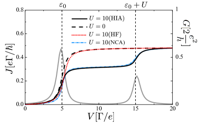
Figure 1: Current versus voltage for $\mu_{R}=0,\mu_{L}=V,\,\varepsilon_{0}=5,\,U=10,\,T=0.1,\,\Gamma_{L}=\Gamma_{R}=0.5$, in the Hubbard I approximation, non interacting case, Hartree-Fock and noncrossing approximations (see text). The differential conductance (y axis on the right side) for HIA is also shown in gray.

There are two jumps in $J(V)$ which correspond to $V=\varepsilon_{0}$ and $V=\varepsilon_{0}+U$. One might think that $U$ lowers the current, as seen in Fig. 1. However, it is not a general result: the Coulomb repulsion can even raise it, as observed in the upper part of Fig. 2 and more obviously in the lower part. For the parameters used in these figures, a simple expression for the current, valid in the weak coupling limit ($\Gamma\ll U,V$)

$$J=\frac{e\Gamma}{\hbar}\frac{1}{2}\Bigl{(}(1-n_{\sigma})(f_{L}-f_{R})_{\varepsilon_{0}}+n_{\sigma}(f_{L}-f_{R})_{\varepsilon_{0}+U}\Bigr{)},$$ (55)

associated with a weak-coupling expression for density $n_{\sigma}=(1-n_{\bar{\sigma}})\displaystyle\bar{f}(\varepsilon_{0})+n_{\bar{\sigma}}\displaystyle\bar{f}(\varepsilon_{0}+U)$, enables to evaluate the current plateau values observed in the three plots. The proximity between HIA and weak-coupling predictions for bias corresponding to the middle of the plateaus is smaller than 5%. However the transition between two consecutive plateaus is too abrupt in the weak-coupling approach due to its delta-shaped spectral weight. $J$ increases with the number of conducting channels opened in the bias window, but not in proportion with this number. Indeed the Hubbard band spectral weight renormalizes each contribution, as explicitly stated in Eq. (55).

To further validate the foundations of our approach, that is HIA out of equilibrium, to which the formalism reduces under steady-state conditions, we compare its predictions for the current with those evaluated within a more sophisticated approach, namely NCA. In NCA on-dot interaction is treated in a more reliable way than in HIA and the spectral density displays a more elaborate structure: showing at low temperature the Kondo resonance, and more generally wider Hubbard bands (typically four times wider). Thus for a quantitative comparison, we choose NCA parameters such as to obtain the same peak locations and bandwidths in both approaches rem . As can be seen in Figs. 1 and 2, we obtain an overall satisfying agreement between NCA and HIA. Even for the considered temperature $T=0.1\ \Gamma>T_{K}$, where $T_{K}$ is the Kondo temperature, some discrepancies can be observed, especially for $\epsilon_{0}=0$, because of the incipient Kondo resonance. However NCA slightly overestimates the Kondo resonance weight when this structure is close to $\epsilon_{0}$ WingreenMeir1994 .

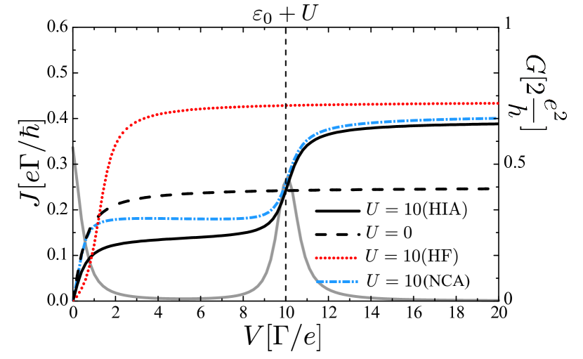
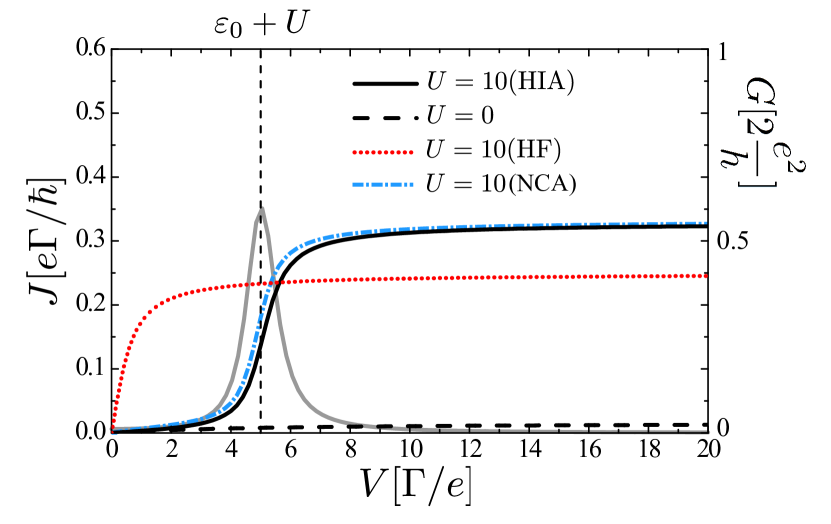
Figure 2: Same as Fig.1, but with $\varepsilon_{0}=0$ (top) and $\varepsilon_{0}=-5$ (bottom).

V Time-dependent case

In the time-dependent case it is necessary to solve Eqs. (LABEL:eq:final1)-(LABEL:eq:final2), with $\Sigma^{r}(t_{1},t_{2})$ given by Eq. (LABEL:eq:sigmar).

V.1 Wide-band limit

It is possible to go further analytically in the case of the wide-band limit, that is neglecting the influence of bandstructure details: in that case $\rho(\varepsilon_{k})$ is assumed to be independent of $\varepsilon_{k}$ and the couplings to the leads become $V_{k\alpha}(t)=u_{\alpha}(t)V_{\alpha}$ where $V_{\alpha}$ are constant. This leads to $\Gamma^{L/R}(\varepsilon,t,t^{\prime})=\Gamma^{L/R}(t,t^{\prime})$, and the retarded self-energy becomes

$$\Sigma^{r}(t,t^{\prime})=-\frac{i}{2}\Gamma(t)\delta(t-t^{\prime}),$$ (56)

where $\Gamma(t)\equiv\sum_{\alpha}\Gamma^{\alpha}(t,t)=2\pi\rho\sum_{\alpha}u_{\alpha}^{2}(t)|V_{\alpha}|^{2}\equiv\sum_{\alpha}\Gamma^{\alpha}u_{\alpha}^{2}(t)$. It is then possible to solve the equations for the retarded Green’s functions

$$\tilde{G}_{\sigma\sigma,0(U)}^{r}(t,t^{\prime})=g_{0(U)}^{r}(t,t^{\prime})\exp\left\{-\int_{t^{\prime}}^{t}\frac{\Gamma(t_{1})}{2}dt_{1}\right\}.$$ (57)

The expressions for $g_{0(U)}^{r}(t,t^{\prime})$ were given previously in Eqs. (21) and (22). The total retarded Green’s function is then determined from Eq. (36).

It is worth noting that the analytical simple expression quoted in Eq. (57) which is very convenient for numerical evaluation, is a direct consequence of the original manner used in this work to make the Hubbard I approximation. With the canonical HIA, we do not obtain such a handy result.

The lesser Green’s function can be evaluated using the Langreth analytic continuation rules, see Eq. (37). To calculate the lesser Green’s functions it is useful to define, following Ref JauhoWingreenMeir1994

$$A_{L/R}^{0(U)}(\varepsilon,t) = \int dt_{1}u_{L/R}(t_{1})\tilde{G}_{\sigma\sigma,0(U)}^{r}(t,t_{1})e^{i\varepsilon(t-t_{1})}$$ (58)

$$\times\exp\left(-i\int_{t}^{t_{1}}dt_{2}\Delta_{L/R}(t_{2})\right).$$

Using these functions it is possible to write the lesser Green’s function in a compact form

$$G_{\sigma\sigma}^{<}(t,t) = in_{\sigma}(t)$$ (59)

$$= i\sum_{L,R}\Gamma^{L/R}\int\frac{d\varepsilon}{2\pi}f_{L/R}(\varepsilon)\left\{\left[1-n_{\bar{\sigma}}(t)\right]|A_{L/R}^{0}(\varepsilon,t)|^{2}\right.$$

$$+\left.n_{\bar{\sigma}}(t)|A_{L/R}^{U}(\varepsilon,t)|^{2}\right\}.$$

Similarly to the stationary case we have equation for $n_{\sigma}(t)$ which can be solved explicitly to yield

$$n_{\sigma}(t)=n_{\bar{\sigma}}(t)=\frac{n^{0}(t)}{1+n^{0}(t)-n^{U}(t)},$$ (60)

where

$$n^{0(U)}(t) = \sum_{L,R}\Gamma^{L/R}\int\frac{d\varepsilon}{2\pi}\,f_{L(R)}(\varepsilon)|A_{L/R}^{0(U)}(\varepsilon,t)|^{2}.$$ (61)

The current consists of two contributions $J_{L/R}(t)=J_{L/R}^{(1)}(t)+J_{L/R}^{(2)}(t)$, with

$$J_{L/R}^{(1)}(t) = -\frac{e}{\hbar}\Gamma^{L/R}u_{L/R}^{2}(t)\left[n_{\uparrow}(t)+n_{\downarrow}(t)\right],$$ (62)

$$J_{L/R}^{(2)}(t) = -\frac{e}{\hbar}\Gamma^{L/R}u_{L/R}(t)\sum_{\sigma}\int\frac{d\varepsilon}{\pi}f_{L/R}(\varepsilon)$$ (63)

$$\times\mathrm{Im}\left\{B_{L/R}^{0}(\varepsilon,t)+B_{L/R}^{U}(\varepsilon,t)\right\}.$$

Quantities $B_{L/R}^{0(U)}$ appear after the integration of $G_{\sigma\sigma}^{r}$ over $t_{1}$ in the general expression for the current (6). They can be written as

$$B_{L/R}^{0}(\varepsilon,t) = \int dt_{1}[1-n_{\bar{\sigma}}(t_{1})]u_{L/R}(t_{1})\tilde{G}_{\sigma\sigma,0}^{r}(t,t_{1})$$

$$\times e^{i\varepsilon(t-t_{1})}\exp\left(-i\int_{t}^{t_{1}}dt_{2}\Delta_{L/R}(t_{2})\right),$$

$$B_{L/R}^{U}(\varepsilon,t) = \int dt_{1}n_{\bar{\sigma}}(t_{1})u_{L/R}(t_{1})\tilde{G}_{\sigma\sigma,U}^{r}(t,t_{1})$$

$$\times e^{i\varepsilon(t-t_{1})}\exp\left(-i\int_{t}^{t_{1}}dt_{2}\Delta_{L/R}(t_{2})\right).$$

Details of the numerical procedure used for calculation of current for arbitrary time dependences can be found in Appendix A.

V.2 Pulse modulation

In the case of a rectangular pulse shape modulation, we choose the following time dependences

$$\Delta_{L/R}(t) = \left[\operatorname{\theta}(t)-\operatorname{\theta}(t-s)\right]\Delta_{L/R},$$ (66)

$$\varepsilon_{0}(t) = \varepsilon_{0}+\left[\operatorname{\theta}(t)-\operatorname{\theta}(t-s)\right]\Delta,$$ (67)

$$u_{L/R}(t) = 1,$$ (68)

it entails that

$$\Gamma^{L/R}(t) = \Gamma^{L/R}=\frac{1}{2}\Gamma,$$ (69)

$$\Sigma_{\sigma}(t) = -\frac{i}{2}\Gamma.$$ (70)

Figure 3 depicts $J(t)$ and $n_{\sigma}(t)$ for the following choice of parameters: $\Gamma_{L}=\Gamma_{R}=0.5,\,T=0.1,\,\mu_{L}=0,\,\mu_{R}=0,\,\varepsilon_{0}=0,\,\Delta_{L}=10,\,\Delta_{R}=0,\,\Delta=5$, $s=3$, for $U=0$, and $U=10$ (HF and HIA), in $\Gamma$ unit for energy and $\hbar/\Gamma$ unit for time. For finite $U$ in the HIA the current behaves similarly as in the case of no correlations, experiencing ringing (pseudo-oscillations) with the same period, but with reduced value when the transient regime fades. The HF approximation predicts a period which is roughly half as long. A higher current value for $U=0$ than for $U=10$ can be explained as follows: for $U=10$, only one channel corresponding to the energy transition $\varepsilon_{0}+\Delta$ lies in between $\mu_{L}+\Delta_{L}$ and $\mu_{R}+\Delta_{R}$ ($\varepsilon_{0}+\Delta+U$ is outside the bias window) while for $U=0$ both channels contribute to the current.

The similarity between the non-interacting case and the HIA, as well as the discrepancy between these and the HF result is also obvious in the dot occupancy versus time plot (lower part of Fig. 3). For $U=0$, $\epsilon_{0}(t)$ always lies in the middle of the bias window, then by symmetry $J_{L}(t)=-J_{R}(t)$, such that the dot occupancy is not affected by the bias step: $n_{\sigma}$ is therefore time-independent, and equals 1/2. The dot occupancy in the HIA is neither affected by the bias onset for the same reason, and the obtained constant value of 1/3 can be understood on time-independent grounds. This value attests the spectral weight transfer which takes place between the two Hubbard bands: indeed the weight of the lower Hubbard band is $1-n_{\bar{\sigma}}$, furthermore this band lies symmetrically around the middle of the bias window, for which $\bar{f}(\epsilon)=1/2$, such that one has $1/2(1-n_{\bar{\sigma}})=n_{\sigma}$, hence leading to the value $n_{\sigma}=1/3$. The occupancy in HF approach at $t=0$ is reduced compared to the non-interacting one due to the shift of the band towards higher energy. Conversely and in an erroneous way, the HF result for $n_{\sigma}$ is time-dependent and brings up an artificial characteristic time scale. Quite generally charge conservation leads to

$$J_{L}(t)+J_{R}(t)-e\sum_{\sigma}\frac{dn_{\sigma}}{dt}=0\ ,$$ (71)

where the first two terms are tunnel currents, while the last one is called displacement current. Thus a time-independent dot occupancy is expected when, by symmetry, $J_{L}(t)=-J_{R}(t)$.

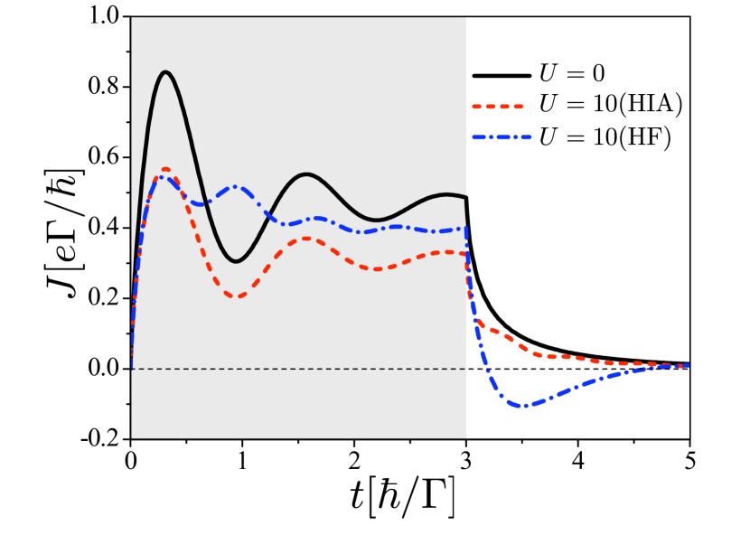
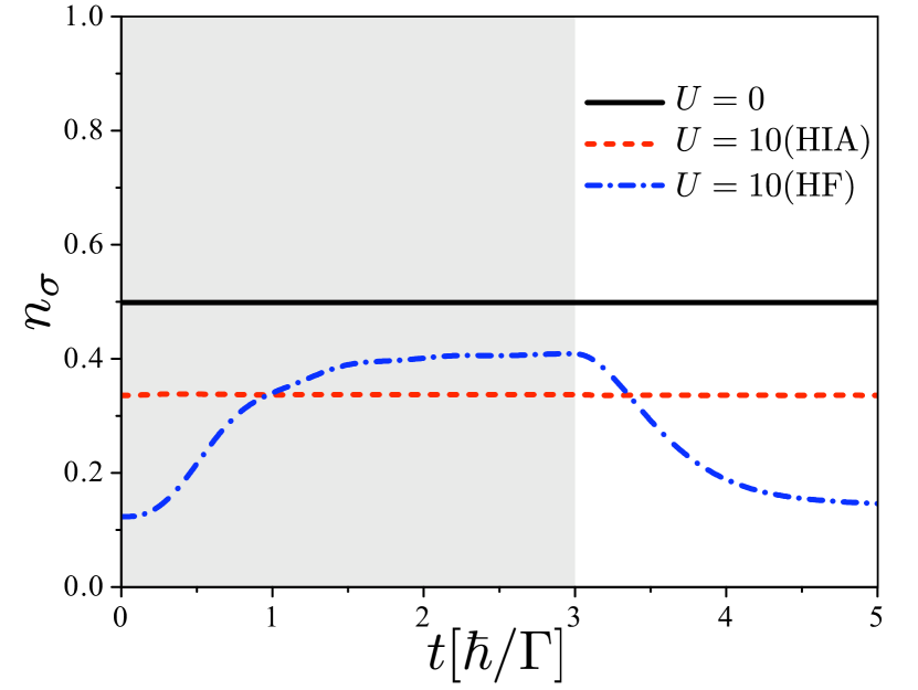
Figure 3: Time dependence of current (top) and occupancy per spin at the dot (bottom) in case of pulse modulation with $\Gamma_{L}=\Gamma_{R}=0.5,\,T=0.1,\,\mu_{L}=0,\,\mu_{R}=0,\,\varepsilon_{0}=0,\,\Delta_{L}=10,\,\Delta_{R}=0,\Delta=5$, $s=3$, for $U=0$ and $U=10$ (HF and HIA). The gray area depicts the pulse duration.

When both bands lie in the bias window, as in Fig. 4, the differences for current and occupancy between $U=0$ and HIA for $U=10$ are attenuated. As previously noted, the periods of pseudo-oscillations of $J(t)$ are nearly the same between $U=0$ and HIA, while the amplitudes are slightly different. Now the density is affected by the bias setup, even for $U=0$, due to an asymmetric distribution of spectral weight in the bias window.

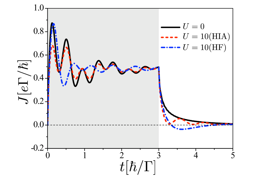
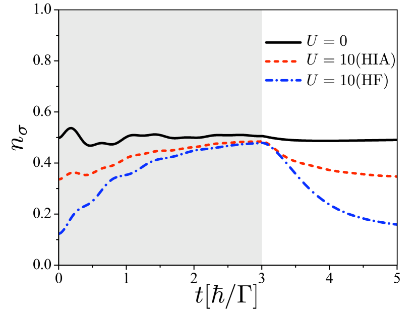
Figure 4: Same as Fig.3, but for $\Delta_{L}=20$.

All these results, for one or two bands inside the bias window, display a transient regime which differs depending on whether the bias is turned on or off. The greatest qualitative difference between non-interacting and HIA results occurs during the equilibrium restoration. We observe that the over-current values are quite close in HF and HIA in Fig. 3, but it may be fortuitous: it is not the case in Fig. 4. The HF has an additional shortcoming, predicting a temporary sign reversal of the current immediately after the pulse end, a behavior absent in the HIA and non interacting cases, which can be attributed in part to an overestimation of the dot occupancy in the steady state regime combined with an underestimation of $n_{\sigma}$ in the equilibrium regime. Finally we choose the voltages and local dot parameters in such a way as to visualize the Coulomb blockade - conducting transition. This is shown in Fig. 5 where, at $t=0$ the dot leaves the insulating Coulomb blockade region to enter the conducting one until $t=s$. Letting $s\rightarrow\infty$ enables to access the charging time of the dot: for the present parameters, using an exponential modelization, we find $\tau\sim 1.2\ \hbar/\Gamma$ in HIA, this is about twice as long as the time predicted by HF, as seen in Fig.  5.

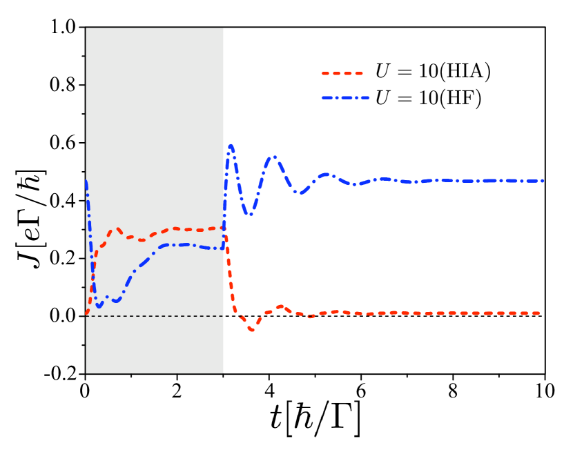
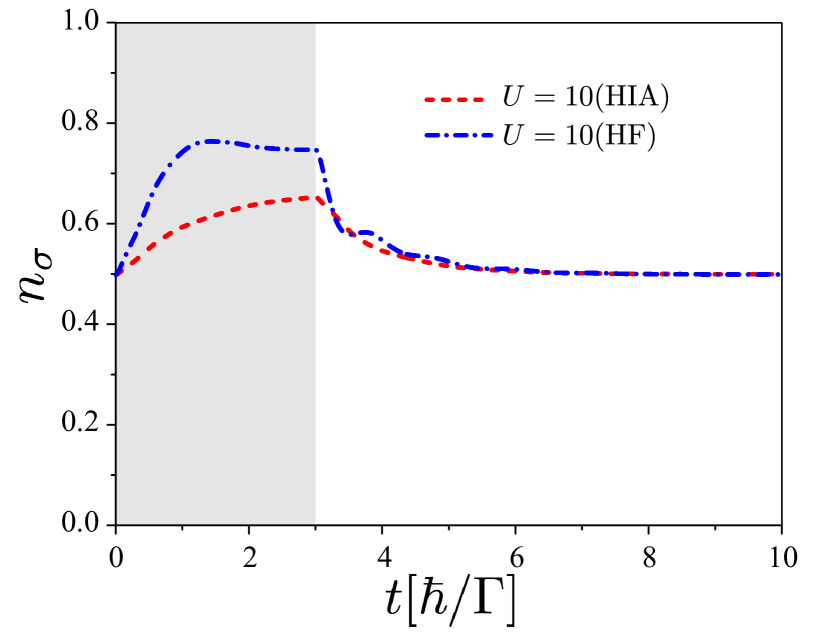
Figure 5: Same as Fig.3, but for $\mu_{L}=10\ ,\varepsilon_{0}=-5\ ,\Delta_{L}=0\ ,\Delta=-10$.

To explore further the discrepancies between HF and HIA, we analyze the dependence on $U$ of the transferred charge or time-integrated symmetrized current. The interval between consecutive pulses is assumed to be much larger than the length of the pulse, therefore we can treat consecutive pulses independently. Since the length of the pulse $s$ is less than time duration of the transient regime (see Figs. 3-4), this charge $Q$ can illustrate properties of purely time-dependent phenomena, it is shown in Fig. 6.

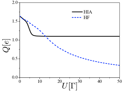
Figure 6: Transferred charge per pulse versus $U$ in HF and HIA, for $\mu_{L}=\mu_{R}=0,\ \varepsilon_{0}=0,\ T=0.1,\ \Delta_{L}=10,\ \Delta_{R}=0,\ \Delta=5,\ s=3$.

For small $U$, both HF and HIA give the same result, as expected since they converge to the exact description for $U=0$. In the HIA, increasing $U$ from 0, the transferred charge $Q$ decreases to settle at a constant value when the higher Hubbard band leaves the bias window. The value $U=5$ which corresponds to $\varepsilon_{0}+\Delta+U=\mu_{L}+\Delta_{L}$, marks the upturn between $U=0$ and $U\rightarrow\infty$ regimes. The smoothness of this decrease depends on $\Gamma$. Besides, in the HF approximation, the charge transferred $Q$ keeps decreasing with the increase of $U$. The Hubbard I approximation is known to contain more physics than HF approximation, e.g. in stationary and equilibrium cases, and we can conclude that HF approximation is also insufficient to describe time-dependent transport in presence of Coulomb repulsion myohaetal .

It is interesting to explore which parameters can influence the period of the “ringing” in the time-dependence of $J(t)$. When we change all the parameters $\Delta_{L}$, $\Delta_{R}$ and $\Delta$, the time-dependence can be rather complicated (see Fig. 4), so we can focus on only one parameter. Let us fix the values of $\Delta_{R}$ and $\Delta$ to zero and change only $\Delta_{L}$. Figure 7 depicts $J(t)$ in case of a step-function characterized by $\Gamma_{L}=\Gamma_{R}=0.5,\,T=0.1,\,\mu_{L}=0,\,\mu_{R}=0,\varepsilon_{0}=0,\,U=10,s\to\infty$, and with $\Delta_{L}=15,30,45$.

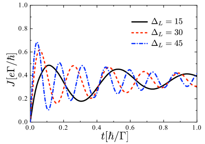
Figure 7: $J(t)$ in case of step voltage for different values of $\Delta_{L}$, for $\mu_{L}=\mu_{R}=0,\ \varepsilon_{0}=0,\ U=10,\ T=0.1,\ \Delta_{R}=\Delta=0,\ s\geq 1$.

The value of the steady-state current does not change with $\Delta_{L}$: indeed in all cases the conducting channels are the same. In the meantime, the period is strongly affected by $\Delta_{L}$: the product of $\Delta_{L}$ and period $T_{0}$ approximately satisfies $\Delta_{L}\cdot T_{0}\sim 2\pi$. This can be attributed to the presence of a phase multiplier of the form $\exp(i\Delta(t^{\prime})t^{\prime})$ in the expressions which determine the time dependence of the current. This result is compatible with the observation reported in Ref myohanenepl098 where the oscillations are ascribed to the electronic transitions between the lower dot state and the leads potentials.

Finally we can also study the temperature influence on $J(t)$. Figure 8 depicts $J(t)$ for different $T$ values.

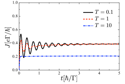
Figure 8: $J(t)$ in case of step voltage for different temperatures, for $\mu_{L}=\mu_{R}=0,\ \varepsilon_{0}=0,\ U=10,\ \Delta_{L}=20,\ \Delta_{R}=\Delta=0,\ s\geq 5$.

Moderate temperature has little influence on “ringing” period, but can change significantly the amplitude of these oscillations. Besides, very high temperature affects the steady-state value of the current, which is attained almost instantaneously. So, it is seen that complex time-dependence is restricted to low temperatures.

V.3 Harmonic modulation

It is interesting to explore the case when external voltages are periodic in time and how correlations, after the transient regimes, influence the forced ones. In case of harmonic modulation we choose in-phase voltages: $\Delta_{L/R,0}(t)=\Delta_{L/R,0}\cos(\omega t)$. This kind of modulation was studied before for the non-interacting case in Ref. JauhoWingreenMeir1994 and in Ref. CroySaalmann86 with an exponential modulation of the hybridization; it was generalized to the interacting model in the HF approximation Deus2012 . Such an harmonic time-dependence was also adressed in the Kondo regime Lopez1998 Arrachea2008 . Figure 9 depicts the time dependence of the current (top) and dot occupancy per spin (bottom) in case of harmonic modulation, for the following parameters: $\Gamma_{L}=\Gamma_{R}=0.5,\,T=0.1,\,\mu_{L}=10,\,\mu_{R}=0,\,\varepsilon_{0}=5,\,\Delta_{L}=10,\,\Delta_{R}=0,\Delta=5$, $\omega=2$ (pulsation measured in $\Gamma/\hbar$), for $U=0$ and $U=10$ (HF and HIA).

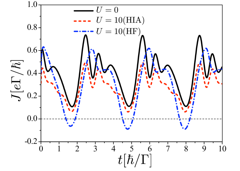
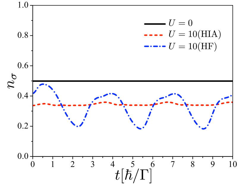
Figure 9: Time dependence of current (top) and dot occupancy per spin (bottom) in case of harmonic modulation, for $\Gamma_{L}=\Gamma_{R}=0.5,\,T=0.1,\,\mu_{L}=10,\,\mu_{R}=0,\,\varepsilon_{0}=5,\,\Delta_{L}=10,\,\Delta_{R}=0,\Delta=5$, $\omega=2$, for $U=0$ (exact solution) and $U=10$.

In HIA, the modulation amplitude for dot occupancy is very slight, but not strictly zero: it stays close to 1/3, and never reaches 2/5, which would be expected once per period, if the system were adiabatic. Eventually, in this forced regime, the current becomes periodic in time, with the same period as the external perturbation. For the chosen parameters, a rise and fall regime sets in: the higher Hubbard band alternatively reaches the border and leaves the varying bias window. However a higher frequency (about three times larger) also emerges.

As also previously argued, the HF approximation is not reliable in the transient regime, not more in the forced regime, predicting a periodic current inversion, as well as a poor estimation of dot occupancy.

V.4 Adiabatic and non-adiabatic pumping

As previously mentioned in the harmonic regime, current and densities do not follow adiabatic predictions, even at low frequency $\hbar\omega\leq\Gamma$ Cavaliere09 . The non-adiabatic behavior is exploited in charge pumping. The idea of producing a current in the absence of any bias voltage, called pure pumping, can also be addressed within the HIA. A recent paper focussed on this issue in a formalism close, but not equivalent, to the present work CroySaalmann85 . These authors truncate the hierarchy of equation of motion at the same level than detailed above, and manage also to circumvent double-time Green’s functions evaluation, using an auxiliary-mode expansion. It thus seemed to us interesting to make a detailed comparison between these two resembling techniques. In the footsteps of these authors, we looked at the case of a gaussian pulse gate voltage, and calculated the left current. Results are shown in Fig. 10. Varying the gaussian time-width $t_{p}$ allows to browse the cases of adiabatic and non adiabatic response. There is a qualitative agreement, and a very good quantitative consistency for rapid pulse (low $t_{p}$); however some discrepancies in the adiabatic region are observed, the current being higher in our HIA. The origin of this difference in not very clear for us but stems from different correlation treatment procedures; indeed for $U=0$ our numerical procedure for arbitrary time dependence was checked by a detailed comparison with Jauho’s et al. results JauhoWingreenMeir1994 , we also agree with uncorrelated Croy et al.’s results.

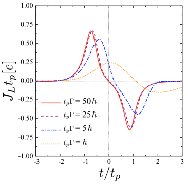
Figure 10: Left current versus time for a gaussian-time-dependent gate voltage $\varepsilon_{0}(t)=1-2e^{-(t/t_{p})^{2}}$, in the HIA for different values of $t_{p}$, the other parameters are $\mu_{R}=\mu_{L}=0,\,U=10,\,T=0.1,\,\Gamma_{L}=\Gamma_{R}=0.5$.

VI Conclusions

A time-dependent formalism for a single level interacting quantum dot coupled to two leads has been developed within the Hubbard I approximation, in a convenient and handy way for numerical evaluation. It enables us to consider general time dependences for hybridization as well as for gate or bias voltages. To validate the approach, the steady-state regime has been, in some parameter range, favorably compared with NCA results.

The formalism results in the appearance of two Hubbard bands in the local spectral density. For those bands we introduce two Green’s functions, which offer the key advantage to get rid of double-time evaluation, without any a priori assumption about adiabatic or sudden limits. These bands undergo spectral weight transfers which influence the transport properties, in contrast with the rigid band frame.

Calculations show the influence of Coulomb correlations on the current, which mainly consists in a change of amplitude. The influence on the time structure (e.g. “ringing” period), appear to be mostly insignificant. Comparisons between Hubbard I and Hartree-Fock approximations show that the latter is insufficient to describe time-dependent transport.

The presented method can also be extended beyond the wide band limit, indeed the key point consists in writing the dot Green’s function as a sum of two independent Green’s functions; this acts upstream, before the assumption of wide band limit. To implement our formalism beyond this limit deserves further study.

Appendix A: Numerical procedure

Here we describe the numerical procedure used for calculating the current and the dot occupancy for arbitrary time dependences in the wide-band limit for the HIA. The time dependences are $\Delta_{L(R)}(t)$, $\varepsilon_{0}(t)=\varepsilon_{0}+\Delta(t)$, $u_{L(R)}(t)$ with the only condition being that all time-dependent perturbations start at $t_{0}$. For the sake of simplicity we choose in this appendix $t_{0}=0$, i.e. for $t<0$ we have a stationary state. The time-dependent current and dot occupancy are calculated by integrating the $A_{L(R)}^{0(U)}(\varepsilon,t)$ and $B_{L(R)}^{0(U)}(\varepsilon,t)$ functions. The key point here is the numerical computation of these functions.

We will split the integration, e.g. in the expression (58) for $A_{L(R)}^{0(U)}$ into two parts: $\int_{-\infty}^{t}=\int_{-\infty}^{0}+\int_{0}^{t}$. Then, after performing the integration in the first term we get

$$A_{L/R}^{0(U)}(\varepsilon,t)=\frac{\exp\left[i(\varepsilon-\varepsilon_{0(U)})t\right]}{\varepsilon-\varepsilon_{0(U)}+\frac{i\Gamma}{2}}$$

$$\times\exp\left[-i\int_{0}^{t}dt_{1}\left(\Delta(t_{1})-\Delta_{L(R)}(t_{1})-\frac{i\Gamma(t_{1})}{2}\right)\right]$$

$$-i\int_{0}^{t}dt_{1}\exp\left[i\varepsilon(t-t_{1})\right]u_{L/R}(t_{1})\exp\left[-i\int_{t_{1}}^{t}dt_{2}\varepsilon_{0(U)}(t_{2})\right]$$

$$\times\exp\left[i\int_{t_{1}}^{t}dt_{2}\Delta_{L/R}(t_{2})\right]\exp\left[-\int_{t_{1}}^{t}\frac{\Gamma(t^{\prime})}{2}dt^{\prime}\right].$$ (72)

Expressions for $B_{L/R}^{0(U)}$ are also expressed in this form, for instance we get

$$B_{L/R}^{0}(\varepsilon,t)=\frac{(1-n_{\bar{\sigma}}^{0})\exp\left[i(\varepsilon-\varepsilon_{0})t\right]}{\varepsilon-\varepsilon_{0}+\frac{i\Gamma}{2}}$$

$$\exp\left[-i\int_{0}^{t}dt_{1}\left(\Delta(t_{1})-\Delta_{L(R)}(t_{1})-\frac{i\Gamma(t_{1})}{2}\right)\right]$$

$$-i\int_{0}^{t}dt_{1}\left(1-n_{\bar{\sigma}}(t_{1})\right)\exp\left[i\varepsilon(t-t_{1})\right]u_{L/R}(t_{1})$$

$$\times\exp\left[-i\int_{t_{1}}^{t}dt_{2}\varepsilon_{0}(t_{2})\right]\exp\left[i\int_{t_{1}}^{t}dt_{2}\Delta_{L/R}(t_{2})\right]$$

$$\times\exp\left[-\int_{t_{1}}^{t}\frac{\Gamma(t^{\prime})}{2}dt^{\prime}\right],$$ (73)

where $n_{\bar{\sigma}}^{0}$ is the stationary value prior to modulation.

At $t=0$ we can compute the stationary current and occupancy. We have

$$A_{L/R}^{0(U)}(\varepsilon,0) = \frac{1}{\varepsilon-\varepsilon_{0(U)}+\frac{i\Gamma}{2}},$$ (74)

$$B_{L/R}^{0}(\varepsilon,0) = \frac{(1-n_{\bar{\sigma}}^{0})}{\varepsilon-\varepsilon_{0}+\frac{i\Gamma}{2}},$$ (75)

$$B_{L/R}^{U}(\varepsilon,0) = \frac{n_{\bar{\sigma}}^{0}}{\varepsilon-\varepsilon_{0}-U+\frac{i\Gamma}{2}},$$ (76)

from which we can compute $n_{\sigma}^{0}$ and then $J^{0}$, using Eqs. (60)-(63).

To compute transport properties for $t>0$, we express $A_{L/R}^{0(U)}(\varepsilon,t+dt)$ using Eq. (72) in terms of $A_{L/R}^{0(U)}(\varepsilon,t)$ at previous time step:

$$A_{L/R}^{0(U)}(\varepsilon,t+dt)=A_{L/R}^{0(U)}(\varepsilon,t)\exp\left(i(\varepsilon-\varepsilon_{0(U)})dt\right)\times$$

$$\exp\left[-i\int_{t}^{t+dt}dt_{1}\left(\Delta(t_{1})-\Delta_{L(R)}(t_{1})-\frac{i\Gamma(t_{1})}{2}\right)\right]$$

$$-i\int_{t}^{t+dt}dt_{1}\exp\left[i\varepsilon(t+dt-t_{1})\right]u_{L/R}(t_{1})\times$$

$$\exp\left[-i\int_{t_{1}}^{t+dt}dt_{2}\varepsilon_{0(U)}(t_{2})\right]\times\exp\left[i\int_{t_{1}}^{t+dt}dt_{2}\Delta_{L/R}(t_{2})\right]$$

$$\exp\left[-\int_{t_{1}}^{t+dt}\frac{\Gamma(t^{\prime})}{2}dt^{\prime}\right].$$ (77)

Because $dt$ is small we can use the midpoint method to perform integration from $t$ to $t+dt$

$$A_{L/R}^{0(U)}(\varepsilon,t+dt)\approx A_{L/R}^{0(U)}(\varepsilon,t)\exp\left(i(\varepsilon-\varepsilon_{0(U)})dt\right)$$

$$\times\exp\left[-idt\left(\Delta(\tilde{t})-\Delta_{L(R)}(\tilde{t})-\frac{i\Gamma(\tilde{t})}{2}\right)\right]$$

$$-idt\exp\left[i\varepsilon\frac{dt}{2}\right]u_{L/R}(\tilde{t})$$

$$\times\exp\left[-i\frac{dt}{2}\left(\varepsilon_{0(U)}(\tilde{\tilde{t}})-\Delta_{L/R}(\tilde{\tilde{t}})-\frac{i\Gamma(\tilde{\tilde{t}})}{2}\right)\right],$$ (78)

where $\tilde{t}=t+\frac{dt}{2}$ and $\tilde{\tilde{t}}=t+\frac{3dt}{4}$.

For $B_{L/R}^{0(U)}$ it is possible to obtain similar approximation but $n_{\bar{\sigma}}$ also appears in the integration from $t$ to $t+dt$. We will use $n_{\bar{\sigma}}\left(t+\frac{dt}{2}\right)\approx\displaystyle{\frac{1}{2}\left(n_{\bar{\sigma}}(t)+n_{\bar{\sigma}}\left(t+dt\right)\right)}$. Indeed we can compute $n_{\bar{\sigma}}\left(t+dt\right)$ before computing $B_{L/R}^{0(U)}(\varepsilon,t+dt)$ because it is determined only by $A_{L/R}^{0(U)}$. In the end, we get, e.g. for $B_{L/R}^{0}$

$$B_{L/R}^{0}(\varepsilon,t+dt)\approx B_{L/R}^{0}(\varepsilon,t)\exp\left(i(\varepsilon-\varepsilon_{0})dt\right)$$

$$\times\exp\left[-idt\left(\Delta(\tilde{t})-\Delta_{L(R)}(\tilde{t})-\frac{i\Gamma(\tilde{t})}{2}\right)\right]$$

$$-idt\frac{2-n_{\bar{\sigma}}(t)-n_{\bar{\sigma}}\left(t+dt\right)}{2}\exp\left[i\varepsilon\frac{dt}{2}\right]u_{L/R}(\tilde{t})$$

$$\times\exp\left[-i\frac{dt}{2}\left(\varepsilon_{0}(\tilde{\tilde{t}})-\Delta_{L/R}(\tilde{\tilde{t}})-\frac{i\Gamma(\tilde{\tilde{t}})}{2}\right)\right].$$ (79)

Computing and integrating the central quantities $A_{L(R)}^{0(U)}(\varepsilon,t)$ and $B_{L(R)}^{0(U)}(\varepsilon,t)$ in the previously presented calculations, typically require less than one minute on a 1.7 GHz Core 2 Duo.

References

- (1) For an early review of the field see, Mesoscopic Phenomena in Solids, edited by B.L. Altshuler, P.A. Lee, and R.A. Webb (Elsevier, Amsterdam, 1991).
- (2) S. Datta, Quantum Transport: Atom to Transistor (Cambridge University Press, Cambridge, 2005).
- (3) H. Haug and A.-P. Jauho, Quantum Kinetics in Transport and Optics of Semiconductors (Springer, Berlin, 2007).
- (4) J. Appenzeller and D.J. Frank 2004 Appl. Phys. Lett. 84, 1771
- (5) Z. Zhong, N.M. Gabor, J.E. Sharping, A.L. Gaeta, and P.L. McEuen 2008 Nature Nanotechnology 3 201
- (6) A.P. Jauho, N.S. Wingreen, Y. Meir 1994 Phys. Rev. B 50 5528
- (7) D. Kienle and F. Léonhard 2009 Phys. Rev. Lett. 103 026601
- (8) P. Nordlander, M. Pustilnik, Y. Meir, N.S. Wingreen, and D.C. Langreth 1999 Phys. Rev. Lett. 83 808
- (9) M. Plihal, and D.C. Langreth, and P. Nordlander 2000 Phys. Rev. B 61 R13341
- (10) J. Hubbard 1963 Proc. R. Soc. Lond. A 276 238
- (11) A.C. Hewson 1966 Phys. Rev. 144 420
- (12) A. Croy, U. Saalmann, A.R. Hernández, C.H. Lewenkopf 2012 Phys. Rev. B 85 035309
- (13) N. E. Bickers, D. L. Cox, and J. W. Wilkins 1987 Phys. Rev. B 36 2036
- (14) P. Myöhänen, A. Stan, G. Stefanucci, R. vanLeeuwen 2009 Phys. Rev. B 80 115107
- (15) J. Splettstoesser, M. Governale, J. König, and R. Fazio 2005 Phys. Rev. Lett. 95 246803
- (16) P.W. Anderson 1961 Phys. Rev. 124 41
- (17) L.V. Keldysh 1965 Sov. Phys. JETP 20 1018
- (18) To obtain similar bandwidths in NCA and HIA, we choose four times smaller in NCA.
- (19) N.S. Wingreen and Y. Meir 1994 Phys. Rev. B 49 11040
- (20) P. Myöhänen, et al. 2008 Eur. Phys. Lett. 84 670001
- (21) A. Croy, U. Saalmann 2012 Phys. Rev. B 86 035330
- (22) F. Deus, A.R. Hernandez, and M.A. Continentino 2012 J. Phys: Condens. Matter 24 356001
- (23) R. López, R. Aguado, G. Platero, and C. Tejedor 1998 Phys. Rev. Lett. 81 4688
- (24) L. Arrachea, A. Levy Yeyati, and A. Martin-Rodero 2008 Phys. Rev. B 77 165326
- (25) F. Cavaliere, M. Governale, and J. König 2009 Phys. Rev. Lett. 103 136801