Transfer matrix analysis of one-dimensional majority cellular automata with thermal noise

Abstract

Thermal noise in a cellular automaton refers to a random perturbation to its function which eventually leads this automaton to an equilibrium state controlled by a temperature parameter. We study the 1-dimensional majority-3 cellular automaton under this model of noise. Without noise, each cell in this automaton decides its next state by majority voting among itself and its left and right neighbour cells. Transfer matrix analysis shows that the automaton always reaches a state in which every cell is in one of its two states with probability 1/2 and thus cannot remember even one bit of information. Numerical experiments, however, support the possibility of reliable computation for a long but finite time.

1 Introduction

In theoretical computer science, reliable computation in the presence of noise has been attracting researchers since von Neumann’s work on the fault-tolerance of Boolean circuits in 1956 [1]; a faultless circuit was simulated by a circuit of noisy gates that is larger only by logarithmic factor and performs the same computation with some constant probability of success close to one. In his simulation, the fault-tolerance mainly stems from majority voting and redundancy: each intermediate result is computed several times and its value is determined to be the one supported at least by half. Non-uniform connectivity among gates is also important in order to obtain fault-tolerance [2, 3, 4].

The possibility to manufacture systems with homogeneous components and advances in parallel computation call for the study of fault-tolerance in models with uniform structure. The cellular automaton (CA), introduced by Ulam [5] and von Neumann [6], is one of them. A CA is a regular array of cells, where each cell can be in two or more states, and computes a function of its neighbouring cells at discrete time steps $t$. Fault-tolerance of CA has been investigated under various noise models [7, 8, 9], but mainly subject to the flip noise which, regardless of the computation, affects the output of a cell (e.g. inverts its binary output with some probability $\epsilon$).

In statistical physics (SP), studies of CA go back to Wolfram [10], who studied the behaviour of CA by simulations and analytically. The CA model of Wolfram is a deterministic limit of more general probabilistic CA (PCA) [8]. A large class of PCA satisfies the detailed balance condition for some Hamiltonian (energy) function [11]. Hence as $t\rightarrow\infty$, they are governed by a stationary distribution of the Gibbs-Boltzmann type. The question of fault-tolerance is then directly related to the occurrence of phase transitions, i.e. the presence of several stationary distributions [12], in infinite size systems. Furthermore, a more general scenario can be treated by mapping non-equilibrium distributions of PCA into equilibrium SP models [13, 14].

In this paper, we study the fault-tolerance of the 1-dimensional majority-3 cellular automaton (1d-MAJ3-CA) with thermal noise. The 1d-MAJ3-CA is a 1-dimensional array of identical 2-state cells. The state of a cell is updated by taking the majority vote among itself and its left and right neighbour cells. Thermal noise disturbs the computation in the gates by adding a random term proportional to the temperature parameter $T$. Although the flip noise makes the result of a computation surely incorrect once it takes place, the thermal noise does nothing beyond competing with it, and hence, even if it occurs, the computational result can still be correct. Here, using the transfer matrix method [15], we show that, as long as the temperature is positive, the thermal noise eventually leads the 1d-MAJ3-CA to the equilibrium state in which each cell is in one of its two states with probability 1/2. In other words, it cannot “remember one bit of information” forever (Gacs discussed this problem for the flip noise [7] and stated analogous results).

This paper is organised as follows. We define the model in section 2. In section 3, we present numerical simulations, and use the transfer matrix method in section 4 to study the equilibrium properties of this model. Finally, in section 5 we summarise and discuss our results.

2 Model

The 1d-MAJ3-CA consists of $N$ cells interacting on the 1-dimensional lattice, with periodic boundary. The state of the $i$-th cell at time $t$ is denoted by the Ising variable $s_{i}(t)\in\{-1,1\}$. The configuration $s(t)=(s_{1}(t),\ldots,s_{N}(t))$ of the CA is the assignment of a state (-1 or 1) to each cell. The dynamics is governed by the synchronous stochastic alignment process

$$s_{i}(t+1)=\textrm{sgn}\left[h_{i}(s(t))+T\eta_{i}(t)\right],$$ (1)

where the local field $h_{i}(s(t))$ is given by $h_{i}(s(t))=s_{i-1}(t)+s_{i}(t)+s_{i+1}(t)$, and sgn is the sign function defined as $\textrm{sgn}[x]=+1$ for $x\geq 0$ and $\textrm{sgn}[x]=-1$ for $x<0$. The noise, represented by $\eta_{i}(t)$, is competing with the local field. Its amplitude is controlled by the temperature parameter $T\in[0,\infty)$. For $T=0$, the process (1) converts into a deterministic majority-3 voting, while for $T\rightarrow\infty$ it is completely driven by noise.

Let us assume that $\eta_{i}(t)$ are independent and identically distributed random variables coming from the distribution

$$\mathrm{P}(\eta)=\frac{1}{2}\left[1-\tanh^{2}(\eta)\right].$$ (2)

Under this distribution of noise, the process (1) leads us to the probability law

$$\mathrm{P}[s_{i}(t+1)|s(t)]=\frac{1}{2}\left[1+s_{i}(t+1)\tanh\left(\beta h_{i}(s(t))\right)\right],$$ (3)

where $\beta=1/T$ is the inverse temperature. This model of noise was used in studies of neural networks [16, 17], and of metastablity in PCA  [18].

Given a configuration $s(t)$ at time $t$, the configuration $s(t+1)$ at time $t+1$ is governed by the probability $\mathrm{W}[s(t+1)|s(t)]=\prod_{i=1}^{N}\mathrm{P}[s_{i}(t+1)|s(t)]$. This is a transition probability of the Markov process

$$\mathrm{P}_{t+1}(s) = \sum_{\hat{s}}\mathrm{W}[s|\hat{s}]\mathrm{P}_{t}(\hat{s}),$$ (4)

which traces the evolution of the probability $\mathrm{P}_{t}(s)$ to find the variables in a state $s$ at time $t$.

The choice (2) for the noise distribution guarantees that the system (4) has a unique [16] stationary solution

$$\mathrm{P}_{\infty}(s)=\frac{1}{\mathrm{Z}}\prod_{i=1}^{N}2\cosh(\beta h_{i}(s)),$$ (5)

where $\mathrm{Z}=\sum_{s}\prod_{i=1}^{N}2\cosh(\beta h_{i}(s))$ is the partition function. This distribution can be also written in a more familiar (equilibrium) Gibbs-Boltzmann form $\mathrm{P}_{\infty}(s)=\mathrm{e}^{-\beta E(s)}/\mathrm{Z}$ upon definition of the “energy” function $E(s)=-\frac{1}{\beta}\sum_{i=1}^{N}\log 2\cosh(\beta h_{i}(s))$ (this is not a proper energy function, or Hamiltonian, because of its explicit dependence on the noise parameter $\beta$). Furthermore, for the probabilistic majority-3 automaton, the choice of (2) is the only type of noise which guarantees the convergence to Gibbs-Boltzmann equilibrium [11].

Finally, let us compare the thermal noise model (3) with the flip-noise model

$$\mathrm{P}[s_{i}(t+1)|s(t)]=\frac{1}{2}\left[1+s_{i}(t+1)\,\textrm{sgn}\left[h_{i}(s(t))\right]\tanh(\tilde{\beta})\right],$$ (6)

which corresponds to the process $s_{i}(t+1)=\xi_{i}(t)\,\textrm{sgn}\left[h_{i}(s(t))\right]$, where $\xi_{i}(t)\in\{-1,1\}$ and $\mathrm{P}(\xi_{i}(t)=-1)=[1-\tanh(\tilde{\beta})]/2$. The probability of an error ($s_{i}(t+1)\,\textrm{sgn}\left[h_{i}(s(t))\right]=-1$) in this model, and in the thermal noise model, is given by the functions $[1-\tanh(\tilde{\beta})]/2$ and $[1-\tanh(\beta|h_{i}(s(t))|)]/2$, respectively. Suppose that one of these models is in the ordered state, and the probability of an error in the other model is not higher than in this one. Then intuitively, both models are in the ordered state. This intuition turns out to be correct for models with non-uniform topologies [19, 20], but whether this is true in a more general case is not clear.

3 Monte-Carlo simulations

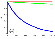
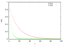
Figure 1: Remembering 1-bit of information by the 1d-MAJ3-CA automaton with $N=10^{6}$ cells in the presence of noise with temperature $T$. Left: $T=\{0.5,0.75,1.0\}$ (from top to bottom). Right: $T=\{2.0,3.0\}$ (from top to bottom).

In this section, we show with Monte-Carlo (MC) simulations of the process (1), starting from the configuration with all cells in the state $+1$, that the 1d-MAJ3-CA automaton of finite size can remember this one bit of information for a considerable amount of time, even at relatively high temperatures. As McCann and Pippenger point out in [9]: “this property of remembering a bit is all that is needed to achieve fault-tolerant computation.”

In Figure 1, we plot the magnetization $m(s(t))=\frac{1}{N}\sum_{i=1}^{N}s_{i}(t)$ measured in the MC simulation of $N=10^{6}$ cells evolving in time $t$ for low and high temperatures. Here the state $m(s(t))=1$ means that the system holds 1-bit of information by having all its cells in the state $+1$, whereas if $m(s(t))=0$, then half of the cells are in $+1$ and the other half are in $-1$, i.e., the information is lost. We note that even after $10^{4}$ time-steps, more than $90\%$ of the cells of the 1d-MAJ3-CA are in the correct state $+1$ at $T=0.75$. Further analysis of the dynamics is required in order to say how quickly the information about the initial state of the automaton gets lost.

4 Transfer matrix analysis of the equilibrium

The equilibrium probability distribution (5) can be used to compute thermal averages such as $\langle s_{i}\rangle=\sum_{s}\mathrm{P}_{\infty}(s)s_{i}$ and $\langle s_{i}s_{j}\rangle=\sum_{s}\mathrm{P}_{\infty}(s)s_{i}s_{j}$. The former will allow us to show that the 1d-MAJ3-CA indeed forgets its initial configuration after a long time, and the latter will allow us to study correlations. Let us first consider the partition function

$$Z = \sum_{s_{1},\ldots,s_{N}}\prod_{i=1}^{N}2\cosh(\beta(s_{i-1}+s_{i}+s_{i+1}))$$ (7)

where $s_{0}=s_{N}$ and $s_{1}=s_{N+1}$ (periodic or closed boundary). In order to compute this function, we will use the transfer-matrix method [15].

To this end, we consider an auxiliary two-cell binary-state automaton, whose state diagram is presented in Figure 2. This diagram gives rise to the ”transition” matrix

$$\mathbf{T}=\left(\begin{array}[]{cccc}2\cosh(3\beta)&2\cosh(\beta)&0&0\\ 0&0&2\cosh(\beta)&2\cosh(\beta)\\ 2\cosh(\beta)&2\cosh(\beta)&0&0\\ 0&0&2\cosh(\beta)&2\cosh(3\beta)\end{array}\right),$$ (12)

where rows and columns are labelled by the binary vectors $(+1;+1)$, $(+1;-1)$, $(-1;+1)$ and $(-1;-1)$, in this order. An element of this matrix is defined by $\mathbf{T}[s_{i},s_{j}|s_{k},s_{l}]=2\cosh(\beta(s_{i}+s_{j}+s_{l}))\delta_{s_{j};s_{k}}$, where $\delta_{s_{j};s_{k}}$ is the Kronecker delta. After $N$ “time-steps”, the state of this automaton is governed by the operator $\mathbf{T}^{N}$. Now due to the properties of the matrix $\mathbf{T}$, we have

$$\Tr(\mathbf{T}^{N}) = \sum_{s_{1},...,s_{N}}\sum_{s_{1}^{\prime},...,s^{\prime}_{N}}\prod_{i=1}^{N}\mathbf{T}[s_{i-1},s_{i}^{\prime}|s_{i},s_{i+1}^{\prime}]$$

$$= \sum_{s_{1},...,s_{N}}\prod_{i=1}^{N}\mathbf{T}[s_{i-1},s_{i}|s_{i},s_{i+1}]=Z.$$

Thus $\mathbf{T}$ is a transfer matrix for the original majority-3 system. This construction can be used to obtain a transfer matrix for any one-dimensional majority voting system where the vote concerns $2k+1$ cells (the central cell and $k$ neighbours to the left and to the right of this cell). However, the dimensionality of the transfer matrix grows exponentially with $k$ (see A).

Figure 2: Transition diagram of the auxiliary two-cell binary-state automaton, with $w_{3}=2\cosh(3\beta)$ and $w_{1}=2\cosh(\beta)$.

For majority-3, we note first that the transfer matrix $\mathbf{T}$ has four distinct eigenvalues and can be diagonalised as $\mathbf{P}^{-1}\mathbf{T}\mathbf{P}=\mathbf{D}$. $\mathbf{D}$ is a diagonal matrix constructed from the eigenvalues

$$\lambda_{1,3} = \frac{1}{2}\left(w_{3}+w_{1}\pm\sqrt{(w_{3}-w_{1})^{2}+4w_{1}^{2}}\right)$$ (14)

$$\lambda_{2,4} = \frac{1}{2}\left(w_{3}-w_{1}\pm\sqrt{(w_{3}+w_{1})^{2}-4w_{1}^{2}}\right)$$

of $\mathbf{T}$, where $w_{3}=2\cosh(3\beta)$ and $w_{1}=2\cosh(\beta)$. $\mathbf{P}$ is the matrix whose columns are the corresponding eigenvectors of $\mathbf{T}$. Then using the properties of the trace, we obtain $Z=\lambda_{1}^{N}+\lambda_{2}^{N}+\lambda_{3}^{N}+\lambda_{4}^{N}$. In the thermodynamic limit $N\to\infty$, the partition function $Z$ is dominated by the largest eigenvalue $\lambda_{1}=\left(w_{3}+w_{1}+\sqrt{(w_{3}-w_{1})^{2}+4w_{1}^{2}}\right)/2$ for any finite $\beta$.

Let us now compute local magnetisations and correlations. To this end, we use the relation

$$P_{\infty}(s)=\sum_{\tilde{s}}W[s|\tilde{s}]P_{\infty}(\tilde{s}),$$ (15)

which expresses the invariance of the equilibrium distribution. All sites are equivalent because of the periodic boundary, hence it is sufficient to consider the average magnetization $\left<s_{1}\right>=\sum_{s}P_{\infty}(s)s_{1}$ at site $1$. Using the identity (15), we obtain

$$\left<s_{1}\right>=\sum_{\tilde{s}}\tanh(\beta h_{1}(\tilde{s}))P_{\infty}(\tilde{s}).$$ (16)

Now

$$\left<s_{1}\right> = \frac{1}{Z}\sum_{s}\tanh\left(\beta h_{1}(s)\right)\prod_{i=1}^{N}2\cosh\left(\beta h_{i}(s)\right)$$ (17)

$$= \frac{1}{Z}\sum_{s}2\sinh\left(\beta h_{1}(s)\right)\prod_{i=2}^{N}2\cosh\left(\beta h_{i}(s)\right)$$

$$= \frac{\Tr(\mathbf{S}\mathbf{T}^{N-1})}{\Tr(\mathbf{T}^{N})},$$

where

$$\mathbf{S}=\left(\begin{array}[]{cccc}2\sinh(3\beta)&2\sinh(\beta)&0&0\\ 0&0&2\sinh(\beta&-2\sinh(\beta)\\ 2\sinh(\beta)&-2\sinh(\beta)&0&0\\ 0&0&-2\sinh(\beta)&-2\sinh(3\beta)\end{array}\right).$$ (22)

Finally, defining the matrix $\mathbf{M}=\mathbf{P}^{-1}\mathbf{S}\mathbf{P}$, we obtain

$$\left<s_{1}\right>=\frac{\sum_{i=1}^{4}\mathbf{M}_{i,i}\lambda_{i}^{N-1}}{\sum_{i=1}^{4}\lambda_{i}^{N}}.$$ (23)

In the thermodynamic limit, $\lim_{N\to\infty}\left<s_{1}\right>=\mathbf{M}_{1,1}/\lambda_{1}$. However, $\mathbf{M}_{1,1}=0$ (see B) and thus $\left<s_{i}\right>=0$ for all $i$ at any finite $\beta$, i.e. the system is in a disordered (paramagnetic) state.

Let us now compute the correlations $\left<s_{i}s_{j}\right>=\sum_{s}P_{\infty}(s)s_{i}s_{j}$ for $j>i$. Using the equilibrium relation (15) and following the steps of (17), we obtain

$$\left<s_{i}s_{j}\right> = \frac{\Tr(\mathbf{T}^{i-1}\mathbf{S}\mathbf{T}^{j-i-1}\mathbf{S}\mathbf{T}^{N-j})}{\Tr(\mathbf{T}^{N})}$$ (24)

$$= \frac{\Tr(\mathbf{M}\mathbf{D}^{j-i-1}\mathbf{M}\mathbf{D}^{N+i-j-1})}{\Tr(\mathbf{T}^{N})}$$

$$= \frac{\sum_{k,l=1}^{4}\mathbf{M}_{k,l}\lambda_{l}^{j-i-1}\mathbf{M}_{l,k}\lambda_{k}^{N+i-j-1}}{\sum_{k=1}^{4}\lambda_{k}^{N}}$$

In the thermodynamic limit $N\to\infty$, this equation reduces to

$$\left<s_{i}s_{j}\right> = \sum_{k=1}^{4}\frac{\mathbf{M}_{1,k}\mathbf{M}_{k,1}}{\lambda_{1}^{2}}\left(\frac{\lambda_{k}}{\lambda_{1}}\right)^{j-i-1}$$ (25)

$$= \left<s_{i}\right>\left<s_{j}\right>+\sum_{k=2}^{4}\frac{\mathbf{M}_{1,k}\mathbf{M}_{k,1}}{\lambda_{1}^{2}}\left(\frac{\lambda_{k}}{\lambda_{1}}\right)^{j-i-1}.$$

However, $\mathbf{M}_{1,3}=0=\mathbf{M}_{3,1}$ (see B) and $\left<s_{i}\right>=0$ for all $i$. Thus

$$\left<s_{i}s_{j}\right> = \frac{\mathbf{M}_{1,2}\mathbf{M}_{2,1}}{\lambda_{1}\lambda_{2}}\left(\frac{\lambda_{2}}{\lambda_{1}}\right)^{j-i}+\frac{\mathbf{M}_{1,4}\mathbf{M}_{4,1}}{\lambda_{1}\lambda_{4}}\left(\frac{\lambda_{4}}{\lambda_{1}}\right)^{j-i}.$$ (26)

Furthermore, it can be shown that

$$\frac{\mathbf{M}_{1,2}\mathbf{M}_{2,1}}{\lambda_{1}\lambda_{2}}+\frac{\mathbf{M}_{1,4}\mathbf{M}_{4,1}}{\lambda_{1}\lambda_{4}}=1,$$ (27)

so we denote

$$\alpha=\frac{\mathbf{M}_{1,2}\mathbf{M}_{2,1}}{\lambda_{1}\lambda_{2}}$$ (28)

and write

$$\left<s_{i}s_{j}\right> = \alpha\left(\frac{\lambda_{2}}{\lambda_{1}}\right)^{d}+(1-\alpha)\left(\frac{\lambda_{4}}{\lambda_{1}}\right)^{d},$$ (29)

where $d=j-i$.

In the high temperature limit $\beta\to 0$, the ratios $\lambda_{2}/\lambda_{1}$, $\lambda_{4}/\lambda_{1}$ and the function $\alpha$ behave as follows:

$$\frac{\lambda_{2}}{\lambda_{1}} = \beta+\Or(\beta^{2}),$$

$$\frac{\lambda_{4}}{\lambda_{1}} = -\beta+\Or(\beta^{2}),$$

$$\alpha = \frac{1}{2}+\beta+\Or(\beta^{3}).$$ (30)

Thus in this limit,

$$\left<s_{i}s_{j}\right> = \gamma_{d}(\beta+\Or(\beta^{2}))^{d}$$ (31)

where $\gamma_{d}=1+\Or(\beta^{3})$ if $d$ is even and $\gamma_{d}=\beta+\Or(\beta^{3})$ if $d$ is odd. This explains the ”staircase” behavior of the correlation function in Figure 3.

In the low temperature limit $\beta\to\infty$, the function $\alpha\to 1$ and the ratios $\lambda_{2}/\lambda_{1}$, $\lambda_{4}/\lambda_{1}$ behave as follows:

$$\frac{\lambda_{2}}{\lambda_{1}} = 1-2\rme^{-4\beta}+\Or(\rme^{-6\beta}),$$ (32)

$$\frac{\lambda_{4}}{\lambda_{1}} = -\rme^{-2\beta}+\Or(\rme^{-4\beta}).$$

In this limit, and in the large distance limit $d\to\infty$, the correlations decay exponentially as

$$\left<s_{i}s_{j}\right> = \alpha\rme^{-d/\xi},$$ (33)

where $\xi=1/\log(\lambda_{1}/\lambda_{2})$ is a correlation length. This behaviour is illustrated in Figure 3. In the limit $\beta\to\infty$, the correlation length $\xi$ diverges as $\xi\sim\frac{1}{2}\rme^{4\beta}$, identifying $T=0$ as the “critical” temperature of this system – the system is in an ordered (ferromagnetic) state in the limit $T=0$.

It is interesting to compare this behaviour with the conventional one-dimensional Ising case, where $\xi_{\textrm{Ising}}\sim\frac{1}{2}\rme^{2\beta}$ [15]. This comparison shows, as could be expected, that adding a self-interaction, and at the same time increasing the size of the neighbourhood, helps to build correlations in this ferromagnetic system. In addition, the correlation function has at high temperature (and for small distances) an unusual “staircase” behaviour, which is probably due to the parallel dynamics. At lower temperatures, this effect disappears as competing spin domains become larger. It is also instructive to compare this result to the one-dimensional parallel Ising model presented in C. A behaviour depending on the parity of the distance appears also there: the correlation function is zero for odd distances $d=j-i$ (at any temperature), and decreases exponentially with distance $d$ for even distances.

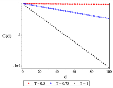
Figure 3: Behaviour of the correlation function $C(d)=\langle s_{0}s_{d}\rangle$ in the 1d-MAJ3-CA predicted by the theory for high and low temperatures $T$. Left: $T=\{0.5,0.75,1\}$. Right: $T=\{2.5,5,10\}$.

5 Discussion

In this paper, we have studied the 1d-MAJ3-CA (1-dimensional majority-3 cellular automaton) in the presence of thermal noise. This allows us to study properties of this automaton with methods of equilibrium statistical physics. In particular, we first formulated the transfer matrix method for a more general 1-dimensional majority-(2k+1) automaton, where $k\geq 1$. This method is exact and allows us to compute the moments of the equilibrium distribution (local magnetization, 2-point correlation, etc.) and various thermodynamic functions such as the free energy, the entropy, etc. for any system of finite size, but also in the thermodynamic limit.

Applying the transfer matrix method to the 1d-MAJ3-CA with periodic boundary leads us to the conclusion that after an infinitely long time, the infinitely large 1d-MAJ3-CA forgets its initial configuration, at any positive (finite) temperature. This result contrasts with the result of [20] for non-uniform (random) topologies, where one bit of information can be remembered in the presence of noise. However, numerical experiments show that the 1d-MAJ3-CA has a quite long memory about its initial state. The same results hold with open boundary – the effect of the boundary is irrelevant in the thermodynamic limit.

An interesting problem for future work is to study the 1d-MAJ(2k+1)-CA (1-dimensional majority-(2k+1) cellular automaton) model for any (finite) $k>1$. This is a difficult problem due to the exponential growth of sizes of matrices used in the transfer matrix method. In the extreme case where $k=N$, the majority automaton reduces to the infinite-range parallel-update Ising model [17], which is fault-tolerant. We should also mention Gács’ construction of a one-dimensional CA [8], which is, to our knowledge, the only one-dimensional fault-tolerant CA known to date. Dynamical studies of the 1d-MAJ3-CA will answer the following questions: how quickly is memory of the initial state lost? And what are the effects of the self-interaction (in (1) the state $s_{i}(t+1)$ is directly dependent on $s_{i}(t)$) on this property of the system? In systems with non-uniform topologies, the presence of self-interaction yields strong memory effects  [20]. A direct approach to this problem is to use the dynamical transfer matrix method [21].

Appendix A Majority-$(2k+1)$

For $k\geq 1$, the majority-$(2k+1)$ cellular automaton (maj-$(2k+1)$ CA) is a 1-dimensional array of $N$ cells $s_{1},\ldots,s_{N}$ with binary states ($-1$ or $1$). Cells’ states are updated synchronously by taking the majority vote among a cell, its $k$ left neighbours, and $k$ right neighbours.

The partition function of maj-$(2k+1)$ CA has the following form:

$$Z=\sum_{s_{1},\ldots,s_{N}}\prod_{i=1}^{N}2\cosh\left(\beta\mbox{$\sum_{j=-k}^{{+k}}s_{i+j}$}\right),$$ (34)

with $s_{-k+1}=s_{N-k+1},\ldots,s_{k}=s_{N+k}$ (periodic boundary conditions).

Figure 4: Majority-5: transition diagram of the auxiliary 4-cell binary-state automaton, with $w_{5}=2\cosh(5\beta)$, $w_{3}=2\cosh(3\beta)$, and $w_{1}=2\cosh(\beta)$.

The transfer-matrix method used in this paper can be applied to the study of the maj-$(2k+1)$ CA. The auxiliary automaton, presented for $k=2$ (majority-5) in Figure 4, is then a $2k$-cell automaton. In other words, the fundamental object is then the state of $2k$ consecutive cells of the maj-$(2k+1)$ CA. This state can have $2^{2k}$ different values, whose list we denote by $(\pm 1,\ldots,\pm 1)_{2k}$, and which we use as indices of the rows and columns of the transfer matrix $\mathbf{T}$. This matrix has then $2^{2k}\times 2^{2k}$ elements $\mathbf{T}[\tilde{s}_{1},...,\tilde{s}_{2k}|\tilde{s}_{2k+1},...,\tilde{s}_{4k}]$, defined in the following way:

$$\mathbf{T}[\ldots|\ldots]=2\cosh\beta\left(\tilde{s}_{1}+\sum_{j=2k+1}^{4k}\tilde{s}_{j}\right)\prod_{\ell=1}^{2k-1}\delta_{\tilde{s}_{\ell+1};\tilde{s}_{2k+\ell}}$$ (35)

So that only $2^{2k+1}$ elements are non-zero. These non-zero elements are presented for $k=2$ by the diagram of Figure 4. Then

$$\Tr(\mathbf{T}^{N}) =\sum_{a_{1},\ldots,a_{N}=(\pm 1,\ldots,\pm 1)_{2k}}\prod_{i=1}^{N}\mathbf{T}_{a_{i},a_{i+1}}$$

$$=\sum_{s_{1},...,s_{N}}\prod_{i=1}^{N}\mathbf{T}[s_{i-k},\ldots,s_{i+k-1}|s_{i-k+1},\ldots,s_{i+k}]$$

$$=Z$$

where $a_{N+1}=a_{1}$ (periodic boundary), and the second equality is due to the properties of $\mathbf{T}$.

Unfortunately, the transfer matrix has a size growing exponentially with $k$, which makes it difficult to diagonalize, even for $k=2$. However, numerical treatment seems to indicate that in this case it still has distinct real eigenvalues of multiplicity one.

Appendix B Matrix $\mathbf{M}$

The matrix $\mathbf{M}=\mathbf{P}^{-1}\mathbf{S}\mathbf{P}$ defined in section 4 has the form

$$\mathbf{M}=\left(\begin{array}[]{cccc}0&\mathbf{M}_{1,2}&0&\mathbf{M}_{1,4}\\ \mathbf{M}_{2,1}&0&\mathbf{M}_{2,3}&0\\ 0&\mathbf{M}_{3,2}&0&\mathbf{M}_{3,4}\\ \mathbf{M}_{4,1}&0&\mathbf{M}_{4,3}&0\\ \end{array}\right).$$ (37)

Defining

$$f(\beta)=\cosh(\beta)\sqrt{2\cosh(4\beta)-8\cosh(2\beta)+10},$$ (38)

we can write the non-zero elements of $\mathbf{M}$ as

$$\mathbf{M}_{1,2}= \frac{\sinh(2\beta)(\cosh(2\beta)+\sinh(2\beta))}{2f(\beta)(\cosh(\beta)+\sinh(\beta))}\times$$

$$\times\big{(}-4\cosh(3\beta)+2\sinh(\beta)+2\sinh(3\beta)-2f(\beta)\big{)},$$

$$\mathbf{M}_{1,4}= -\frac{\sinh(2\beta)(\cosh(\beta)+\sinh(\beta))(\cosh(2\beta)-\sinh(2\beta))}{f(\beta)}\times$$

$$\times\big{(}2\cosh(3\beta)+\sinh(\beta)+\sinh(3\beta)+f(\beta)\big{)},$$

$$\mathbf{M}_{2,1}= -\frac{2\cosh(\beta)(\cosh(\beta)+\sinh(\beta))^{2}}{\cosh(\beta)+\cosh(3\beta)+f(\beta)}\times$$

$$\times\big{(}2\cosh(\beta)-3\sinh(\beta)+\sinh(3\beta)+f(\beta)\big{)},$$

$$\mathbf{M}_{2,3}= -\frac{2\cosh(\beta)(\cosh(\beta)+\sinh(\beta))^{2}}{\cosh(\beta)+\cosh(3\beta)-f(\beta)}\times$$

$$\times\big{(}2\cosh(\beta)-3\sinh(\beta)+\sinh(3\beta)-f(\beta)\big{)},$$

$$\mathbf{M}_{3,2}= -\frac{\sinh(2\beta)(\cosh(2\beta)+\sinh(2\beta))}{f(\beta)(\cosh(\beta)+\sinh(\beta))}\times$$

$$\times\big{(}-2\cosh(3\beta)+\sinh(\beta)+\sinh(3\beta)+f(\beta)\big{)},$$

$$\mathbf{M}_{3,4}= \frac{(\cosh(\beta)-\sinh(\beta))\sinh(2\beta)}{f(\beta)}\times$$

$$\times\big{(}2\cosh(3\beta)+\sinh(\beta)+\sinh(3\beta)-f(\beta)\big{)},$$

$$\mathbf{M}_{4,1}= \frac{\cosh(\beta)(\cosh(\beta)-\sinh(\beta))}{\big{(}\cosh(\beta)+\cosh(3\beta)+f(\beta)\big{)}(\cosh(\beta)+\sinh(\beta))}\times$$

$$\times\big{(}4\cosh(\beta)+6\sinh(\beta)-2\sinh(3\beta)+2f(\beta)\big{)},$$

$$\mathbf{M}_{4,3}= \frac{\cosh(\beta)(\sinh(2\beta)-\cosh(2\beta))}{\cosh(\beta)+\cosh(3\beta)-f(\beta)}\times$$

$$\times\big{(}-4\cosh(\beta)-6\sinh(\beta)+2\sinh(3\beta)+2f(\beta)\big{)}.$$

Appendix C One-dimensional parallel Ising model

The results presented in this work can be also compared with the correlations between cells in the (one-dimensional) parallel Ising model under thermal noise, in which the cell does not refer to itself in the update of its state. Under the noise distribution (2), the parallel Ising model has a unique equilibrium probability distribution

$$\mathrm{P}_{\infty}(s)=\frac{1}{Z}\prod_{i=1}^{N}2\cosh(\beta(s_{i-1}+s_{i+1})),$$ (40)

where $Z=\sum_{s}\prod_{i=1}^{N}2\cosh(\beta(s_{i-1}+s_{i+1}))$. In order to compute the correlation function $\langle s_{i}s_{j}\rangle$, let us rewrite (40) as

$$\mathrm{P}_{\infty}(s) = \frac{1}{Z}\prod_{i=1}^{N}\exp(\ln(\cosh(\beta(s_{i-1}+s_{i+1}))))$$

$$= \frac{1}{Z}\prod_{i=1}^{N}\exp\left(\frac{1}{2}(1+s_{i-1}s_{i+1})\ln\cosh(2\beta)\right)$$

$$= \rme^{\tilde{\beta}N}\frac{1}{Z_{\rm even}}\exp\left(\tilde{\beta}\sum_{i}s_{2i}s_{2i+2}\right)\frac{1}{Z_{\rm odd}}\exp\left(\tilde{\beta}\sum_{i}s_{2i-1}s_{2i+1}\right),$$

where $\tilde{\beta}=\frac{1}{2}\ln\cosh(2\beta)$. The factorization in (C) suggests that the parallel Ising model is actually equivalent to two independent sequential Ising models operating at temperature $1/\tilde{\beta}$. For a sequential Ising model at temperature $1/\tilde{\beta}$, the correlation between cells at distance $d=|i-j|$ is given by $\tanh(\tilde{\beta})^{d}$ [15]. Thus, the correlation $\langle s_{i}s_{j}\rangle$ between cells of the parallel Ising model is equal to $\langle s_{i}s_{j}\rangle=\left(\frac{\cosh(2\beta)-1}{\cosh(2\beta)+1}\right)^{|i-j|}$ when $d=|i-j|$ is even, and it is zero if $d$ is odd.

References

References

- [1] von Neumann J 1956 Probabilistic logics and the synthesis of reliable organisms from unreliable components Automata Studies ed C E Shannon and J McCarthy (Princeton University Press) p 43–98
- [2] Dobrushin R L and Ortyukov S I 1977 Probl. Inf. Transm. 13 201
- [3] Pippenger N 1985 FOCS 1985: the 26th Annual Symposium on Foundations of Computer Science (IEEE) p 30–38
- [4] Spielman D A 1996 FOCS 1996: the 37th Annual Symposium on Foundations of Computer Science (IEEE) p 154–163
- [5] Ulam S 1952 Proceedings of the International Congress of Mathematicians vol 2 (Public School Publishing) p 264–275
- [6] von Neumann J 1966 Theory of Self-Reproducing Automata (University of Illinois Press)
- [7] Gács P 1986 J. Comput. Syst. Sci. 32 15
- [8] Gács P 2001 J. Stat. Phys. 103 45
- [9] McCann M and Pippenger N 2008 J. Comput. Syst. Sci. 74 910
- [10] Wolfram S 1983 Rev. Mod. Phys. 55 601
- [11] Grinstein G, Jayaprakash C and He Yu 1985 Phys. Rev. Lett. 55 2527
- [12] Pra P D, Louis P-Y and Roelly S 2002 ESAIM Probab. Stat. 6 89
- [13] Domany E and Kinzel W 1984 Phys. Rev. Lett. 53 311
- [14] Lebowitz J L, Maes C and Speer E R 1990 J. Stat. Phys. 59 117
- [15] Baxter R J 1982 Exactly Solved Models in Statistical Mechanics (Academic Press)
- [16] Peretto P 1984 Biol. Cybern. 50 51
- [17] Coolen A C C, Kühn R and Sollich P 2005 Theory of Neural Information Processing Systems (Oxford Univerity Press)
- [18] Bigelis S, Cirillo E N M, Lebowitz J L and Speer E R 1999 Phys. Rev. E 59 3935
- [19] Mozeika A, Saad D and Raymond J 2010 Phys. Rev. E 82 041112
- [20] Mozeika A and Saad D 2011 Phys. Rev. Lett. 106 214101
- [21] Coolen A C C and Takeda K 2012 Philos. Mag. 92 64