Metal distributions out to 0.5 $r_{180}$ in the intracluster medium of four galaxy groups observed with Suzaku

Abstract

We studied the distributions of metal abundances and metal-mass-to-light ratios in the intracluster medium (ICM) of four galaxy groups, MKW 4, HCG 62, the NGC 1550 group, and the NGC 5044 group, out to $\sim$ 0.5 $r_{180}$ observed with Suzaku. The Fe abundance decreases with radius, and about 0.2–0.4 solar beyond 0.1 $r_{180}$. At a given radius in units of $r_{180}$, the Fe abundance in the ICM of the four galaxy groups were consistent or smaller than those of clusters of galaxies. The Mg/Fe and Si/Fe ratios in the ICM are nearly constant at the solar ratio out to 0.5 $r_{180}$. We also studied systematic uncertainties in the derived metal abundances comparing the results from two versions of atomic data for astrophysicists (ATOMDB) and single- and two-temperature model fits. Since the metals have been synthesized in galaxies, we collected $K$-band luminosities of galaxies from Two Micron All Sky Survey catalogue (2MASS) and calculated the integrated iron-mass-to-light-ratios (IMLR), or the ratios of the iron mass in the ICM to light from stars in galaxies. The groups with smaller gas mass to light ratios have smaller IMLR values and the IMLR inversely correlated with the entropy excess. Based on these abundance features, we discussed the past history of metal enrichment process in groups of galaxies.

1 Introduction

Clusters and groups of galaxies are the best laboratories for study of their thermal and chemical evolution history governed by baryons. The observations of metals in the intracluster medium (ICM), synthesized by supernovae (SNe) in galaxies give an important clue in studying the evolution of galaxies.

The ratio of the metal mass in the ICM to the total light from galaxies in clusters, the metal-mass-to-light-ratio, is a key parameter in investigating star-formation history in these systems. Using ASCA data, Makishima et al. (2001) summarized iron-mass-to-light-ratios (IMLRs), with the $B$-band luminosity for various objects as a function of their plasma temperature and found that IMLRs in groups are systematically smaller than those in clusters. Using Chandra data, Rasmussen & Ponman (2009) reported that IMLRs of galaxy groups within $\sim 0.5~{}r_{180}$ show a positive correlation with total mass of groups.

Groups of galaxies also differ from richer systems in stellar and gas mass fractions within $r_{500}$ (Lin et al., 2004; Sun et al., 2009; Giodini et al., 2009; Zhang et al., 2011). This dependence on the system mass has been sometimes interpreted that the star-formation efficiency depends on the system mass. The gas-density profiles in the central regions of groups and poor clusters are observed to be shallower and the relative entropy level is higher than the oretical predictions (Ponman et al., 1999, 2003). The entropy profile of the ICM is more expressive characterization of the rmodynamical history than temperature. The excess entropies in poor systems are thought to be caused by non-gravitational processes, likely results of the preheating of central AGN, SNe, and so on, injected the energy to the ICM. The metal distribution in the ICM can be a useful tracer of the history of gas heating in the early epoch, because the relative timing of metal enrichment and heating should affect the present amount and distribution of the metals in the ICM.

The abundance ratios of O, Mg and Si to Fe reflect the relative enrichment from SNe Ia and core-collapse SNe (hereafter SNecc). Using Chandra data, Rasmussen & Ponman (2007) reported that the Si/Fe ratio in the ICM of groups of galaxies increases with radius and the SNecc contribution dominates at $r_{500}$. With Suzaku observations, we can derive the metal abundances of O and Mg beyond cool cores of groups and clusters of galaxies, because the X-ray Imaging Spectrometer (XIS) instrument (Koyama et al., 2007) has a lower background level and higher spectral sensitivity below 1 keV. With Suzaku, the abundance profiles of O, Mg, Si and Fe were derived for several groups and clusters out to $\sim$0.3–0.4 $r_{\rm 180}$ (Matsushita et al., 2007; Komiyama et al., 2009; Sato et al., 2007, 2008, 2009a, 2009b, 2010; Murakami et al., 2011; Sakuma et al., 2011), and, with XMM, Si/Fe ratios were derived out to 0.5 $r_{\rm 180}$ of the Perseus cluster (Matsushita et al., 2013a) and the Coma cluster (Matsushita et al., 2013b). The radial abundance profiles of Mg, Si and S were mostly similar to that of Fe. The number ratio of SNecc and SNe Ia to enrich the ICM is estimated to be $\sim$3 (Sato et al., 2009b, 2010).

In this paper, we describe our study of four galaxy groups, MKW 4, HCG 62, the NGC 1550 group, and the NGC 5044 group, observed out to $\sim 0.5~{}r_{180}$ with Suzaku. MKW 4, the NGC 1550 group, and the NGC 5044 group have central dominant giant elliptical or S0 galaxies. In contrast, the central region ($r<1.1^{\prime}$) of HCG 62 is dominated by three galaxies. All groups have nearly symmetric spatial distributions in the X-ray band (dell’Antonio et al., 1995; Kawaharada et al., 2003; David et al., 1995). Among these systems, results of Suzaku data of HCG 62, the NGC 1550 group, and the NGC 5044 group have already been published out to $0.2~{}r_{180}$ (1 pointing), $0.5~{}r_{180}$ (2 pointings), and $0.3~{}r_{180}$ (3 pointings), respectively (Tokoi et al., 2008; Sato et al., 2010; Komiyama et al., 2009). MKW 4 has been observed with XMM and metal distribution in cool core is reported by O’Sullivan et al. (2003). In this paper, we included six new pointing observations (2 for MKW 4, 1 for HGC 62, 1 for the NGC 1550 group, and 2 for the NGC 5044 group) with Suzaku. In section 2, we summarize the observations and data preparation. Section 3 describes our analysis of the data. In section 4, we summarize the distributions of temperature, the Fe abundance, abundance ratios to Fe, and the IMLR. We discuss our results in section 5.

Recently, atomic data for astrophysicists (ATOMDB), version 2.0.1 which includes major updates of the atomic data and new calculation of lines has been released (Foster et al., 2010). These differences in the atomic data are critical to study metal abundances in the ICM of galaxy groups where Fe-L lines dominate the spectra. In order to compare ATOMDB versions between version 1.3.1 and 2.0.1, we reanalyzed the regions which have been reported with Suzaku using the latest responses and background.

We use Hubble constant $H_{0}=$70 km s^-1 Mpc^-1 in this paper. The solar abundance table is given by Lodders (2003). In this paper, errors are quoted at a 90% confidence level for a single parameter of interest.

2 Observations and Data Reduction

Table 1: Suzaku observation logs and basic properties for four galaxy groups, MKW 4, HCG 62, the NGC 1550 group, and the NGC 5044 group.

Group	Field name	Sequence number		Exposure time		(RA, DEC)a
				ksec		J2000.0
MKW 4	East	805081010		61.8		($12^{\rm h}04^{\rm m}31^{\rm s}.3,+02^{\circ}13^{\prime}44.0^{\prime\prime}$)
	North	805082010		65.0		($12^{\rm h}05^{\rm m}43^{\rm s}.0,+01^{\circ}54^{\prime}20.9^{\prime\prime}$)
HCG 62	Center	800013020		93.8		($12^{\rm h}53^{\rm m}05^{\rm s}.8,-09^{\circ}12^{\prime}07.9^{\prime\prime}$)
	West	805031010		55.9		($12^{\rm h}51^{\rm m}59^{\rm s}.4,-09^{\circ}05^{\prime}01.3^{\prime\prime}$)
NGC 1550	Center	803017010		73.8		($04^{\rm h}19^{\rm m}47^{\rm s}.7,+02^{\circ}24^{\prime}37.8^{\prime\prime}$)
	East	803018010		28.1		($04^{\rm h}20^{\rm m}59^{\rm s}.5,+02^{\circ}24^{\prime}31.0^{\prime\prime}$)
	Northeast	803046010		61.9		($04^{\rm h}20^{\rm m}35^{\rm s}.8,+02^{\circ}36^{\prime}31.0^{\prime\prime}$)
NGC 5044	Center	801046010		19.7		($13^{\rm h}15^{\rm m}24^{\rm s}.1,-16^{\circ}23^{\prime}23.6^{\prime\prime}$)
	15′North	801047010		54.6		($13^{\rm h}15^{\rm m}24^{\rm s}.1,-16^{\circ}08^{\prime}34.8^{\prime\prime}$)
	15′East	801048010		62.4		($13^{\rm h}16^{\rm m}26^{\rm s}.8,-16^{\circ}23^{\prime}16.8^{\prime\prime}$)
	30′North	804013010		56.6		($13^{\rm h}16^{\rm m}23^{\rm s}.8,-15^{\circ}53^{\prime}38.8^{\prime\prime}$)
	30′South	804014010		53.3		($13^{\rm h}14^{\rm m}59^{\rm s}.6,-16^{\circ}51^{\prime}46.4^{\prime\prime}$)
Group	$z$	$\left<kT\right>^{b}$	$N_{H}^{c}$	$D_{L}^{d}$	$r_{180}^{e}$	1 arcmind	(RA, Dec)f
		keV	$10^{20}~{}{\rm cm}^{-2}$	Mpc	Mpc	kpc	J2000.0
MKW 4	0.020	1.8	1.76	87.0	1.18	24.3	($12^{\rm h}04^{\rm m}27^{\rm s}.0,+01^{\circ}53^{\prime}45.0^{\prime\prime}$)
HCG 62	0.0145	1.5	3.31	64.3	1.08	17.8	($12^{\rm h}53^{\rm m}05^{\rm s}.3,-09^{\circ}12^{\prime}01.2^{\prime}$)
NGC 1550	0.0124	1.2	10.2	53.6	0.97	15.2	($04^{\rm h}19^{\rm m}37^{\rm s}.9,+02^{\circ}24^{\prime}36.0^{\prime\prime}$)
NGC 5044	0.0093	1.0	4.87	40.0	0.88	11.5	($13^{\rm h}15^{\rm m}24^{\rm s}.0,-16^{\circ}23^{\prime}07.8^{\prime\prime}$)

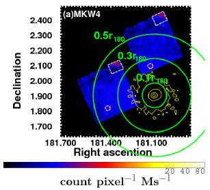
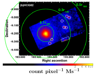
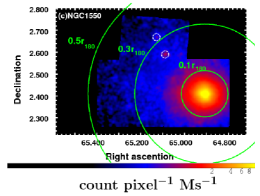
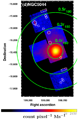
Figure 1: Combined XIS images of (a) MKW 4, (b) HCG 62, (c) the NGC 1550 group, and (d) the NGC 5044 groups in 0.5–2.0 keV. The exposure time was corrected, though vignetting was not corrected. The instrumental backgrounds (NXB) were subtracted. The images were smoothed by a Gaussian of $\sigma=$16 pixels $\approx 17^{\prime\prime}$. The green solid circles correspond to 0.1, 0.3, and 0.5 $r_{180}$. The white dashed circles and boxes show point-like sources and hot pixels, respectively, which were excluded in our analysis. For MKW 4, the X-ray contour map observed with XMM-Newton in logarithm scale from 0.5–2.0 keV are overlaid in yellow.

We selected four galaxy groups, MKW 4, HCG 62, the NGC 1550 group, and the NGC 5044 group, which have been observed up to $0.5~{}r_{180}$ with Suzaku. The observation logs are given in table 1, and the X-ray images in 0.5–2.0 keV are shown in figure 1. The average temperature and the Galactic hydrogen column density for each group are also given in table 1. The virial radius for each group is calculated from the following equation with the average temperature, $r_{180}=1.95(H_{0}/100)^{-1}\sqrt{\langle kT\rangle/10\ \rm keV}$ Mpc (Markevitch et al., 1998; Evrard et al., 1996), and shown in table 1.

In this study, we used only the Suzaku XIS data. The XIS instrument consists of four sets of X-ray CCDs (XIS 0, 1, 2, and 3). XIS 1 is a back-illuminated (BI) sensor, while XIS 0, 2 and 3 are front-illuminated (FI). Because XIS 2 has not been available since 2006 November, all the observations except for the HCG 62 Center and NGC 5044 Center/15^′ East/15^′ North were carried out by XIS 0, 1, and 3. The instruments were operated in the normal clocking mode (8 s exposure per frame) with standard $5\times 5$ or $3\times 3$ editing mode. We used the standard selection data. The analysis was performed by HEAsoft version 6.11 and XSPEC 12.7.0. In the new atomic data (ATOMDB version 2.0.1), the emission line properties have been updated, especially for Fe-L and Ne-K complex lines. These changes would give new results for the temperature and metal abundances in the spectral analysis for the lower temperature system, such as galaxy groups. We, therefore, examined the spectral fits by changing the old (version 1.3.1) or new (version 2.0.1) ATOMDB versions for the same spectra and responses to compare with the previous works. In this paper, the results with the ATOMDB version 2.0.1 are shown unless noted otherwise. We also discuss the difference between the old and new ATOMDB versions in subsection 4.2 in detail.

We generated Ancillary Response Files (ARFs) by “xissimarfgen” Ftools task (Ishisaki et al., 2007), assumed a uniform sky of 20^′ radius. Because the surface brightness profile of the ICM is far from uniform, an ARF file can be generated for an assumed spatial distribution (e.g., $\beta$-model surface brightness profile) on the sky (Ishisaki et al., 2007). However, particularly for offset observations, surface brightness profiles, such as a $\beta$-model profile, which derived from the shape of the central region in the clusters, might not have a good agreement with those in the outer regions. We, therefore, adopted the uniform sky ARFs in our analysis, and estimated the differences of the fit parameters with the $\beta$-model or uniform ARFs as the systematic errors. The resultant fit parameters such as temperatures and abundances, except for the normalizations with the two kinds of ARFs agreed well. As for the normalizations, excluding the innermost region where the effect of the point spread function (PSF) is severe, the difference was within statistical errors. Consequently, those differences were negligible for our results, particularly for the temperature, abundances, and the associated parameters in the outer regions.

The effect of degrading energy resolution by radiation damage was included in the redistribution matrix files by “xisrmfgen” Ftools task. The effect of contaminations on the optical blocking filter (OBF) of the XISs was included in the spectral fits as the photoelectric absorption model ($\it varabs$ model). The C/O ratio of the contaminant was fixed to be 6.0 in number ratio. We employed the night Earth database generated by the “xisnxbgen” Ftools task for the same detector area to subtract the non-X-ray background (NXB).

We searched for point-like sources with “wavdetect” tool in CIAO in 0.5–2.0 keV. As shown by white circles in figure 1, we subtracted the point-like sources with 1^′/1.5^′/2^′ radii. We also excluded the area around the hot pixels as shown in figure 1. The flux level of the faintest source was about 5$\times 10^{-14}$ erg s^-1 cm^-2 in 0.5–2.0 keV with a power-law model of a fixed photon index, $\Gamma=$1.4, and the contribution from unresolved sources were taken into account when we subtracted the Cosmic X-ray Background (CXB) spectrum.

3 Spectral Analysis

We extracted the spectra from annular regions (9^′–13.5^′, 13.5^′–18^′, 18^′–24^′, and 24^′–32^′ for MKW 4; 0^′–3^′, 3^′–6^′, 6^′–13^′, and 13^′–28^′ for HCG 62; 0^′–3^′, 3^′–6^′, 6^′–12^′, 12^′–20^′, and 20^′–30^′ for the NGC 1550 group; 0^′–2^′, 2^′–4^′, 4^′–6^′, 6^′–9^′, 9^′–15^′, 15^′–25^′, 25^′–33^′, and 33^′–42^′ for the NGC 5044 group) as shown in figure 2, centered on the coordinates as shown in table 1. Each spectrum was binned carefully to observe details in metal lines, especially below  1 keV as shown in figure 2. We used the energy ranges, 0.4–7.0 keV and 0.5–7.0 keV for the BI and FI detectors, respectively. We excluded the energy band around the Si-K edge (1.82–1.84 keV) because its response was not modeled correctly. In the spectral fits of BI and FI data, only the normalization parameter was allowed to take different values between them. It is important to estimate the Galactic and CXB emissions accurately, because the spectra, particularly in outer regions of groups, suffer from the Galactic and CXB emissions strongly. We summarizes the background estimations in Appendix A.

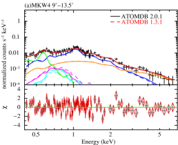
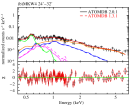
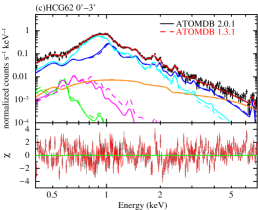
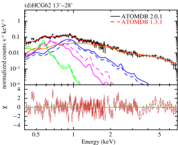
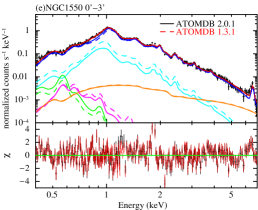
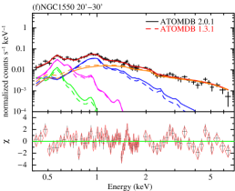
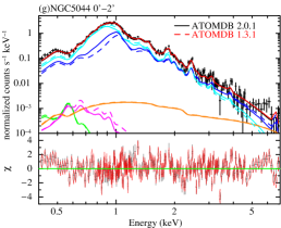
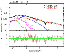
Figure 2: Upper panels show the observed XIS 1 spectra by black crosses. (a) and (b) show the spectra extracted from 9^′–13.5^′ and 24^′–32^′, respectively, for MKW 4. (c) and (d) show the spectra from 0^′–3^′ and 13^′–28^′, respectively, for HCG 62. (e) and (f) show the spectra extracted from 0^′–3^′ and 20^′–30^′ for the NGC 1550 group, respectively. (g) and (h) show the spectra from 0^′–2^′ and 33^′–42^′ for the NGC 5044 group, respectively. Red and black lines indicate the best-fit model with the ATOMDB version 1.3.1 and 2.0.1, respectively. Note that black lines for the best-fit model are completely overlapped by the red lines. The estimated NXB component was subtracted. The hotter and cooler ICM components for the 2T model fits are shown by blue and cyan for the inner regions, and the ICM component for the 1T model fits is indicated by blue for the outermost regions. The CXB, LHB, and MWH components are indicated by orange, green, and magenta lines, respectively. Dashed and solid lines show the best-fit models with the ATOMDB version 1.3.1 and 2.0.1, respectively. The energy band around the Si-K edge (1.82-1.84 keV) is excluded in the spectral fits. The lower panels show the fit residuals in units of $\sigma$.

We assumed that the ICM emission was represented by a single– (hereafter 1T) or two–temperature (hereafter 2T) vapec model (Smith et al., 2001). The metal abundances of He, C, N, and Al were fixed to be a solar value. We divided other metals into six group; O, Ne, Mg, Si, S=Ar=Ca, Fe=Ni, and allowed them to vary. For the 2T model for the ICM, the metal abundances of the two components were assumed to have the same value. We fitted all the spectra with the 1T and 2T models for the ICM with the ATOMDB version 1.3.1 and 2.0.1 for estimating the best-fit model. For HCG 62, the NGC 1550 group, and the NGC 5044 group, we fitted the spectra for each annular region and the outermost region simultaneously for the background constraints as described in Appendix A. The temperature and normalization for each region were allowed to be free, but the abundance of each element was assumed to have the same value. For MKW 4, the spectra from all the annulus regions were fitted simultaneously for constraining the background well.

4 Results

We summarize results of the spectral fits with the ATOMDB version 2.0.1 in subsection 4.1. In this subsection, we show radial profiles of the temperature, normalizations, abundances, and metals to Fe ratios derived from the vapec model. The differences of our results with the old and new ATOMDB versions are mentioned in subsection 4.2. In subsection 4.3, our results are compared with the previous results. Subsection 4.4 describes uncertainties by systematic errors for the background estimations. We derive $K$-band luminosity profiles of the member galaxy for each group from galaxy catalogues in subsection 4.5. In subsection 4.6, we calculate gas mass, iron mass, gas-mass-to-light-ratios (GMLRs), and IMLR profiles.

4.1 Results of spectral fits

We fitted the NXB-subtracted spectra with the 1T and 2T models. All the spectra were well-represented by the 1T or 2T model as shown in figure 2. Figure 3 shows radial reduced $\chi^{2}$ profiles for each spectral fit. The fit statistics in $\chi^{2}$ test significantly favored the 2T model rather than the 1T model within $0.05~{}r_{180}$. In the $r>0.05~{}r_{180}$ region, however, the differences in the reduced $\chi^{2}$ between the 1T and 2T model fits were only several %, and the 1T model represented the observed spectra fairly well. Although the reduced $\chi^{2}$ profiles decreased with radius up to $\sim 0.2~{}r_{180}$, the reduced $\chi^{2}$ in the $r>0.2~{}r_{180}$ had a flatter slope than those in the central region. In the $F$-test probabilities, the spectral fits up to $\sim 0.1~{}r_{180}$ were clearly improved by the 2T model rather than the 1T model. On the other hand, in the $r>0.2~{}r_{180}$, the improvements were not significant.

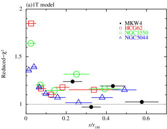
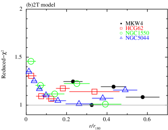
Figure 3: (a) Radial profiles of the reduced $\chi^{2}$ derived from the 1T model fits with the ATOMDB version 2.0.1. (b) The same figure as (a), but from the 2T model fits.

The resultant radial temperature profiles from the 1T and 2T model fits with the ATOMDB version 2.0.1 are shown in figure 4. With the 1T model, the temperatures slightly increased with radius up to $0.1~{}r_{180}$, and it declined to about a half of the peak temperature at $0.5~{}r_{180}$. With the 2T model, within $0.2~{}r_{180}$, the resultant temperatures of both the cooler and hotter components for HCG 62 and the NGC 1550 group decreased with radius. Although the temperature profiles for the NGC 5044 group with the 2T model had larger error bars, the hotter component profile looks similar to that with the 1T model. Beyond $0.2~{}r_{\rm 180}$, we were not able to constrain the temperature of the minor component for the 2T model, and the temperatures of the major component were close to those from the 1T model fits.

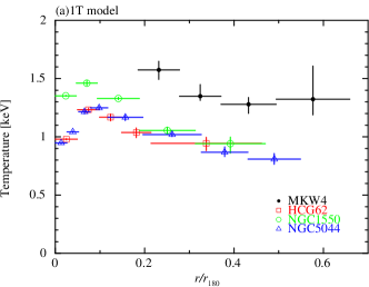
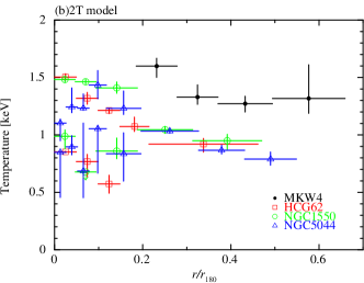
Figure 4: Radial temperature profiles derived from the 1T (left) and 2T (right) model fits. Black, red, green, and blue correspond to the resultant temperatures for MKW 4, HCG 62, the NGC 1550 group, and the NGC 5044 group, respectively. In figure (b), the cooler component in 3^′–6^′ of the NGC1550 group was derived only upper limit.

Figure 5 shows radial profiles of the resultant normalizations, which are derived from the spectral fits with the 1T and 2T models, divided by the area from which each spectrum is extracted. The normalizations divided by the area, which corresponded to the surface brightness profile, decreased with radius for both the 1T and 2T model fits. The normalization profiles for the 1T model fits were close to the sum of those of the cooler and hotter components for the 2T model fits.

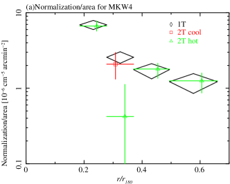
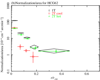
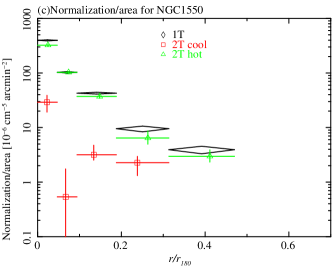
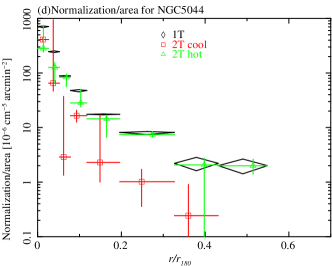
Figure 5: Radial normalization profiles divided by the area for each group. Black diamonds indicate normalization profiles divided by the area with the 1T model. Red squares and green triangles correspond to the normalizations divided by the area of the cooler and hotter components with the 2T model, respectively.

Radial abundance profiles of O, Si, and S derived from the 1T and 2T model fits with the ATOMDB version 2.0.1 are summarized in figure 6. The Mg and Fe abundances within $0.1~{}r_{180}$ had large scatter. Beyond $0.1~{}r_{180}$, the results of all the abundances except for O with both the 1T and 2T model had similar profiles. The O abundance profile showed no radial gradient although the statistical error were fairly large. The Fe abundances decreased with radius, and reached $\sim 0.3$ solar at $0.5~{}r_{180}$.

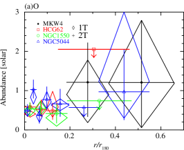
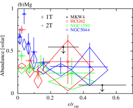
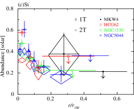
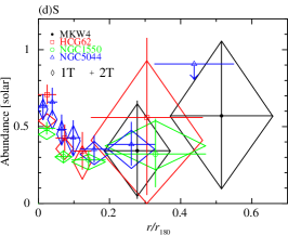
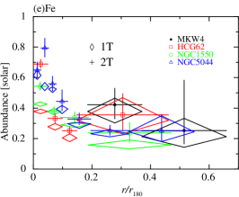
Figure 6: Abundance profiles of (a) O, (b) Mg, (c) Si, (d) S, and (e) Fe in the ICM with the ATOMDB version 2.0.1. The diamonds and crosses indicate the abundances derived from the 1T and 2T model fits, respectively. The notations of colors are same as in figure 3. As for the abundances which were not constrained significantly, here we plotted only the larger upper limit derived from the 1T or 2T model.

We examined radial profiles of the abundance ratios, O/Fe, Mg/Fe, Si/Fe, and S/Fe as shown in figure 7. We do not show Ne/Fe ratio profiles because of large systematic uncertainties for the overlap with strong Fe-L lines. For estimating the abundance ratios rather than the absolute values, we calculated confidence contours between the metal abundances (O, Ne, Mg, and Si) and the Fe abundance. The derived abundance ratios of Mg/Fe, Si/Fe, and S/Fe were consistent to be a constant value of around $\sim 1$, although the error bars were fairly large, particularly in the outer region. Both the 1T and 2T model fits gave similar abundance ratios.

Table 2: Weighted averages of the abundance ratios in units of the solar ratios with ATOMDB version 2.0.1.

group	region	O/Fe [solar ratio]		Mg/Fe [solar ratio]		Si/Fe [solar ratio]		S/Fe [solar ratio]
		1T	2T	1T	2T	1T	2T	1T	2T
MKW 4	Alla	$2.04^{+1.89}_{-1.61}$	$2.04^{+3.10}_{-2.04}$	$0.14^{+0.63}_{-0.14}$	$0.14^{+0.63}_{-0.14}$	$0.76^{+0.74}_{-0.73}$	$0.74^{+0.69}_{-0.69}$	$1.08^{+1.29}_{-1.08}$	$1.05^{+1.19}_{-1.05}$
HCG 62	$<0.1~{}r_{180}$	$1.12^{+0.31}_{-0.30}$	$0.88^{+0.21}_{-0.20}$	$0.87^{+0.13}_{-0.12}$	$1.10^{+0.10}_{-0.10}$	$0.86^{+0.09}_{-0.08}$	$0.86^{+0.07}_{-0.07}$	$1.40^{+0.17}_{-0.17}$	$1.06^{+0.14}_{-0.14}$
	$>0.1~{}r_{180}$	$2.60^{+2.61}_{-1.55}$	$1.89^{+1.14}_{-1.02}$	$0.76^{+0.58}_{-0.58}$	$1.02^{+0.49}_{-0.46}$	$0.86^{+0.40}_{-0.37}$	$0.93^{+0.36}_{-0.33}$	$1.31^{+0.83}_{-0.81}$	$1.36^{+0.78}_{-0.73}$
	Alla	$1.14^{+0.31}_{-0.30}$	$0.92^{+0.21}_{-0.20}$	$0.86^{+0.12}_{-0.12}$	$1.09^{+0.10}_{-0.10}$	$0.86^{+0.08}_{-0.08}$	$0.86^{+0.07}_{-0.07}$	$1.40^{+0.17}_{-0.17}$	$1.07^{+0.13}_{-0.13}$
NGC 1550	$<0.1~{}r_{180}$	$1.25^{+0.41}_{-0.41}$	$1.09^{+0.40}_{-0.37}$	$0.69^{+0.13}_{-0.13}$	$0.81^{+0.13}_{-0.13}$	$0.89^{+0.07}_{-0.07}$	$0.88^{+0.07}_{-0.06}$	$0.98^{+0.09}_{-0.09}$	$0.87^{+0.09}_{-0.09}$
	$>0.1~{}r_{180}$	$1.04^{+1.12}_{-0.55}$	$1.21^{+1.04}_{-0.42}$	$0.96^{+0.32}_{-0.32}$	$1.07^{+0.31}_{-0.31}$	$0.79^{+0.18}_{-0.17}$	$0.77^{+0.17}_{-0.16}$	$0.95^{+0.28}_{-0.28}$	$0.85^{+0.29}_{-0.27}$
	Alla	$1.22^{+0.38}_{-0.33}$	$1.10^{+0.38}_{-0.28}$	$0.73^{+0.12}_{-0.12}$	$0.85^{+0.12}_{-0.12}$	$0.88^{+0.06}_{-0.06}$	$0.87^{+0.06}_{-0.06}$	$0.98^{+0.09}_{-0.09}$	$0.87^{+0.09}_{-0.09}$
NGC 5044	$<0.1~{}r_{180}$	$0.96^{+0.22}_{-0.21}$	$0.98^{+0.23}_{-0.23}$	$1.04^{+0.10}_{-0.10}$	$1.09^{+0.10}_{-0.10}$	$0.69^{+0.06}_{-0.06}$	$0.70^{+0.06}_{-0.06}$	$0.98^{+0.11}_{-0.11}$	$0.90^{+0.11}_{-0.11}$
	$>0.1~{}r_{180}$	$1.73^{+0.84}_{-0.70}$	$1.82^{+1.11}_{-1.17}$	$1.05^{+0.27}_{-0.28}$	$1.17^{+0.32}_{-0.30}$	$0.74^{+0.21}_{-0.20}$	$0.77^{+0.22}_{-0.22}$	$1.18^{+0.38}_{-0.37}$	$1.17^{+0.39}_{-0.38}$
	Alla	$1.03^{+0.22}_{-0.20}$	$1.01^{+0.23}_{-0.22}$	$1.04^{+0.09}_{-0.09}$	$1.10^{+0.10}_{-0.10}$	$0.70^{+0.06}_{-0.06}$	$0.71^{+0.06}_{-0.06}$	$1.00^{+0.10}_{-0.10}$	$0.91^{+0.10}_{-0.10}$

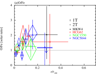
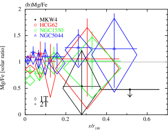
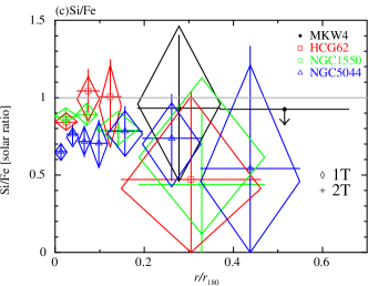
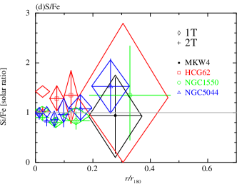
Figure 7: Radial profiles of (a) O/Fe, (b) Mg/Fe, (c) Si/Fe, and (d) S/Fe derived from the spectral fits with the 1T and 2T models with the ATOMDB version 2.0.1. The colors and marks are the same as in figure 3.

We calculated the weighted averages of the abundance ratios derived from both the ATOMDB versions for the $r<0.1~{}r_{180}$, $r>0.1~{}r_{180}$, and whole regions, and summarized in table 2. On the average, the abundance ratios between the $r<0.1~{}r_{180}$ and $r>0.1~{}r_{180}$ regions were almost consistent. The weighted averages of the Mg/Fe, Si/Fe, and S/Fe ratios for the whole regions were consistent to be a solar ratio, although those of the O/Fe ratios had large scatter in the outer regions. The ratios from the 1T and 2T model fits were similar to each other. In addition, the abundance ratios with the ATOMDB version 2.0.1 were consistent with those with the version 1.3.1(table B.1), except for the O/Fe ratios.

4.2 Comparisons of the results with the ATOMDB version 1.3.1 and 2.0.1

In this subsection, we summarize comparisons of the results from the spectral fits with the ATOMDB version 1.3.1 and 2.0.1. Tables and figures are shown in the Appendix B.

In the outer regions, the spectral fits with both the ATOMDB versions gave almost same reduced $\chi^{2}$ (figure B.1). For the 1T model fits, the $\chi^{2}$ values with the ATOMDB version 2.0.1 were smaller than those with the version 1.3.1 within $0.05~{}r_{180}$. On the other hand, the fit statistics in the reduced $\chi^{2}$ favor the ATOMDB version 1.3.1 than the version 2.0.1 with the 2T model within $0.05~{}r_{180}$.

We compared the temperatures derived from the spectral fits with both of the ATOMDB versions (figure B.2 a–c). The resultant temperatures from the 1T model fits and the cooler component from the 2T model fits with the version 2.0.1 were systematically higher than those with the version 1.3.1 by $\sim 0.1$ keV. On the other hand, as for the hotter component of the 2T model fits, the spectral fits with either version gave similar temperatures.

Radial profiles of the normalizations divided by the area from which each spectrum were extracted with the 1T and 2T models were also compared with both the ATOMDB versions (figure B.2 d–f ). As in the temperatures, the resultant normalizations for the 1T model fits and the cooler component for the 2T model fits with the version 2.0.1 were systematically smaller than those with the version 1.3.1. On the other hand, as for the normalizations of the hotter component with the 2T model, the spectral fits with either version also gave similar values.

Figure 8 shows the difference of the derived Fe abundances with the 1T or 2T model between the ATOMDB version 1.3.1 and 2.0.1. The spectral fits with the version 2.0.1 gave significantly smaller Fe abundances than those with the version 1.3.1, particularly within $0.05~{}r_{180}$.

We also compared the abundance ratios of O, Mg, Si, and S to Fe for the 1T and 2T model fits with the version 1.3.1 and 2.0.1, in units of the solar ratios (figure B.3 and B.4 ). The spectral fits with either version gave similar Si/Fe and S/Fe ratios. On the other hand, the spectral fits with the version 2.0.1 gave higher Mg/Fe ratios than those with the version 1.3.1 by 20%. This is because the Mg lines suffer from the Fe-L lines overlapping, and the differences between the ATOMDB versions would cause such systematic differences in the Mg/Fe ratios. The O/Fe ratios with the version 2.0.1 had fairly higher value than those with the version 1.3.1.

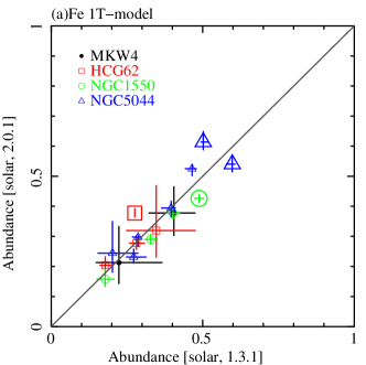
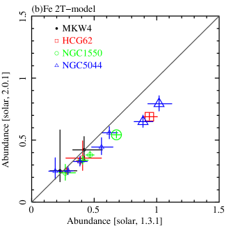
Figure 8: Comparisons of the Fe abundances derived from the 1T and 2T model fits with the ATOMDB version 1.3.1 and 2.0.1. The colors are the same as in figure 3. Bigger marks indicate the Fe abundance and the ratios within $0.05~{}r_{180}$.

4.3 Comparisons of the results with previous results

The temperature and abundance profiles of central regions of our samples, HCG 62, the NGC 1550 group, and the NGC 5044 group, were already reported using XMM, Chandra, and Suzaku data. Therefore, in this subsection, our results using the ATOMDB version 1.3.1 were compared with these previous results, because the previous results were derived with the ATOMDB version 1.3.1 or earlier versions. Here, effects of difference in adopted solar abundance tables were corrected to Lodders (2003). Temperatures and abundances in this work with the ATOMDB version 1.3.1 agreed well with the previous Suzaku results for the NGC 1550 group out to 0.5 $r_{180}$ (Sato et al., 2010), HCG 62 out to 0.2 $r_{180}$ (Tokoi et al., 2008), and the NGC 5044 group out to 0.3 $r_{180}$ (Komiyama et al., 2009).

For the NGC 1550 group, temperatures and abundances with the 1T and 2T model in this work agreed well with the XMM/Chandra results (Sun et al., 2003; Kawaharada et al., 2009) for the whole region observed with the XMM (out to 14^′).

In 6^′–9^′ of HCG 62, temperatures and abundances with the 1T and 2T model in this work were consistent with the Chandra and XMM results (Morita et al., 2006) derived from vMEKAL model (Mewe et al., 1985, 1986; Liedahl et al., 1995; Kaastra, J. S., 1992) fits of deprojected spectra. However, the Fe abundances within 6^′ were significantly smaller and that at 9^′–14^′ were significantly higher than those in Morita et al. (2006). This difference in the inner regions would be caused by the difference in the PSF, in the deprojection and projection, and the adopted atomic codes. The difference in the outer region may be caused by a difference in the treatment of the Galactic foreground emission.

Excluding the innermost region of Suzaku, $r<2^{\prime}$, the temperatures and metal abundances of the NGC 5044 group agreed well with the XMM (Buote et al., 2003a, b) out to $0.2~{}r_{180}$. In the 0.2–0.3 $r_{180}$, the temperature profiles of our results agreed well with Buote et al. (2004). However, our Fe abundances were higher than the XMM abundances by 0.1 solar than that derived with the XMM observations (Buote et al., 2004) ($\sim 0.13$ solar converted to the solar abundance table of Lodders 2003). This difference in the Fe abundances may be caused by the difference in the observed azimuthal directions of the Suzaku (north) and XMM (south). As discussed in Komiyama et al. (2009), the difference in the treatment of the Galactic components may also cause a discrepancy. At the innermost region, $r<2^{\prime}$, of the NGC 5044 group, the temperatures derived from the 1T model and cooler component derived from the 2T model were consistent with the XMM results (Buote et al., 2003a) within the statistical uncertainties, although there were small ($\sim 0.3$ keV) discrepancies for the hotter component of the 2T model fitting. Although our abundances derived from the 1T and 2T models of this region were smaller than the XMM results (Buote et al., 2003b) by several tens of percent, the abundance ratios were consistent each other. When we used the ATOMDB version 1.10, which is used in Buote et al. (2003a, b), the discrepancy in the innermost region became smaller.

The central region of MKW 4 (out to 0.2 $r_{180}$) was observed with XMM (O’Sullivan et al., 2003). The radial temperature profiles outside 0.2 $r_{180}$ in this work smoothly continued the XMM results within 0.2 $r_{180}$. The abundance ratios with XMM were also consistent with our work beyond 0.2 $r_{180}$.

4.4 Uncertainties for the spectral fits

We estimated the systematic errors in our analysis by changing the normalizations of the CXB and the Galactic components by 10%, and the NXB levels by 10% in the spectral fits. As a result, the systematic errors from the background estimations were negligible, and the resultant temperatures and abundances did not change within the statistical errors by changing the background level.

We examined the influence of the uncertainties from the contaminant on the OBF of Suzaku XIS by changing the C/O ratio. We fitted the spectra by changing the C/O ratio to be 12.0 and 3.0, which corresponded to twice and a half of the default composition number ratio, respectively. Consequently, all the parameters except for the O abundance did not changed within the statistical errors. Because C and O absorptions were assumed as the contaminant, O abundance would suffer from the changing ratio. Therefore, we note that the O abundance is not reliably determined because of the contaminant uncertainty in our analysis.

The effect of the PSF and stray light of Suzaku’s X-ray telescope would make photon contaminations from a nearby sky (see also Sato et al. 2007; Urban et al. 2013). In order to estimate the effects, we examined simulations of the contamination flux base on a ray tracing simulator, ”xissim” as shown in Sato et al. (2007). For example, in the case of the NGC 5044, we assumed $\sim 2^{\circ}\times 2^{\circ}$ size of the $\beta$–model surface brightness profile derived from the XMM observations by Nagino et al. (2009) with a 300 ksec exposure time. As a result, the photon fractions originated from each extracted annulus in the outside of 6^′ $\sim 0.1~{}r_{180}$ were 80% and over. On the other hand, although the spectra within 6^′ suffer from the contaminations by $\sim$ 30%, the resultant parameters in the central regions agreed with the previous XMM results within the statistical errors, and they came mostly from the adjacent regions. As for the stray light, we examined the spectral fit in the outermost region including the estimated contamination flux from the bright core in the model. The resultant fit parameters did not change within the statistical errors. Consequently, we proceeded to the spectral analysis without making photon corrections due to the contaminations for the PSF and stray light.

4.5 $K$-band luminosity of galaxies

Table 3: Summary of basic properties for calculating the total $K$-band luminosity within $r_{180}$ for each group.

group	$D_{L}^{a}$	$A_{K}^{b}$	$m_{K}^{c}$	$L_{K,BGD}^{d}$	$L_{K,r_{180}}$
	Mpc			$\times 10^{7}~{}L_{\odot,K}/{\rm arcmin}^{2}$	$\times 10^{12}~{}L_{\odot,K}$
MKW 4	87.0	0.008	7.1	1.72	1.91
HCG 62	64.3	0.016	4.7	2.90	2.13
NGC 1550	53.6	0.050	2.8	2.78	0.73
NGC 5044	40.0	0.026	2.2	0.93	0.82

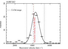
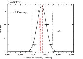
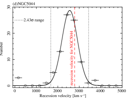
Figure 9: Recession velocity distributions of the galaxies which were identified by the redshift in the catalogues for each group. Black dotted lines indicate $2.43~{}\sigma$ around the means which are close to the recession velocity for each group from NED as shown by red dashed lines.

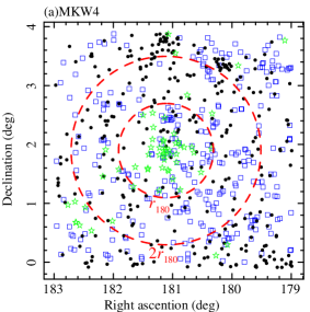
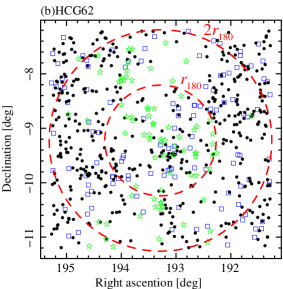
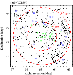
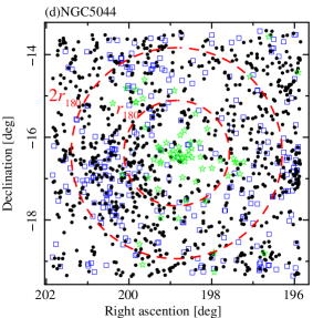
Figure 10: Galaxy distributions for MKW 4, HCG 62, the NGC 1550 group, and the NGC 5044 group in $K$-band from the 2MASS catalogue. Red dashed lines indicate the projected radii of the $r_{180}$ and $2~{}r_{180}$. Green stars and blue boxes indicate member and non-member galaxies, respectively, which are identified by the redshift and recession velocity. Black filled circles indicate the unidentified galaxies by the redshift. (Color version of these figures are available in the online journal.)

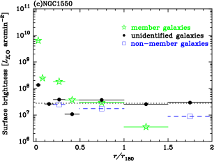
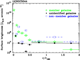
Figure 11: Radial profiles of the surface brightness derived from the $K$-band luminosity of the member galaxies for each group. Green stars, black filled circles, and blue squares correspond to the surface brightness of the member galaxies identified by the redshift in the catalogues, the member galaxies unidentified by the redshift, and non-member galaxies, respectively. Dashed lines indicate the background level derived from the luminosity between the 1 and 2 $r_{180}$ region. For details, see in text.

We investigated radial profiles of the IMLR, which is a useful parameter for a comparison of the ICM metal profiles with the galaxy mass or luminosity distribution, because most metals in the ICM were synthesized in the member galaxies. In order to calculate the IMLR profiles, we derived $K$-band luminosity profiles which well-trace the stellar (galaxy) mass distribution (Nagino et al., 2009), from the Two Micron All Sky Survey (2MASS) catalogue. In the catalogue, we used all of the data in $4^{\circ}\times 4^{\circ}$ region for MKW 4, HCG 62, and the NGC 1550 group, and $6^{\circ}\times 6^{\circ}$ region for the NGC 5044 group, centered on the cD galaxy for each group. We summarize the parameters such as each luminosity distance, the foreground Galactic extinction to calculate the luminosity for each member galaxy, and the appnt magnitude of central galaxy in $K$-band as shown in table 3.

As for an identification of the redshift for each galaxy in the 2MASS catalogue, we assumed an available redshift of each member galaxy as the one by which the galaxy was identified in the Sloan Digital Sky Survey catalogue for MKW 4, in the 6dF Galaxy Survey database for HCG 62 and the NGC 5044 group, and in the 2MASS redshift survey (Crook et al., 2007, 2008) for the NGC 1550 group. As for the galaxies which were identified by the redshift or recession velocity within the projected radius of 2 $r_{180}$, we calculated the recession velocity distribution with 325 km sec^-1 intervals as shown in figure 9, and then obtained the resultant member galaxies which were within $\pm 2.43~{}\sigma$ around the mean. The spacial distributions of the galaxies inside or outside $2.43~{}\sigma$ are shown in figure 10, and the radial profile of the surface brightness are shown in figure 11.

For the galaxies in the 2MASS catalogue which were not identified by the redshift, such as dwarf galaxies, we examined the background subtraction as follows. We derived the surface brightness profile of the galaxies between the projected radius of $r_{180}$ and 2 $r_{180}$. And then, we subtracted the surface brightness level between the $r_{180}$ and 2 $r_{180}$ region as the background from the surface brightness within $r_{180}$ region. The radial profile of the surface brightness up to $r_{180}$ and the background level derived from the 1–2 $r_{180}$ region are shown in figure 11.

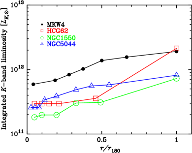
Figure 12: Radial profiles of the integrated $K$-band luminosity (solid lines) for MKW 4, HCG 62, the NGC 1550 group, and the NGC 5044 group. The notations of colors and marks are the same as in figure 3.

As a result, we regarded the sum of the luminosity of the member galaxies which were selected by the redshift and recession velocity, and the galaxies which were not identified by the redshift but for which we performed the background subtraction, as the total luminosity for each group. And then, we calculated radial profiles of the integrated $K$-band luminosity. We next deprojected the luminosity profiles as a function of the radius assuming spherical symmetry, and then derived three-dimensional radial profiles of the integrated $K$-band luminosity up to $r_{180}$ as shown in figure 12 and table 3. Here, even if we took into account the luminosity of dwarf galaxies which were not detected in the 2MASS catalogue, assuming the luminosity function integrated over the magnitude from the cD galaxy to the fully faint-end galaxy for each group, the resultant total $K$-band luminosity within $r_{180}$ would not change by a factor of 2.

4.6 Gas-mass and Iron-mass to light ratio

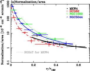
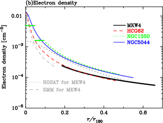
Figure 13: (a) Radial profiles of the normalizations divided by the area from the spectral fits with the 1T model. Solid black and blue, and dashed red lines correspond to the best-fit $\beta$-model for MKW 4, the NGC 5044 group, and HCG 62, respectively. A dotted line is the best fit power-law model for the NGC 1550 group from the normalizations per area. A dotted light gray line shows the surface brightness profile of MKW 4 derived from the previous ROSAT result (Sanderson et al., 2003), which is normalized to the brightness level observed with Suzaku by fitting with the fixed $\beta$ and $r_{c}$ to be 0.64 and 5.45 arcmin, respectively. The notations of colors and marks are the same as in figure 3. (b) Radial profiles of the electron density, $n_{e}$ (cm^-3), derived from the normalizations. Crosses indicate the deprojected electron density derived from the normalizations per area for the NGC 1550 group. Gray dotted and dashed lines indicate the electron density profiles of MKW 4 derived from ROSAT (Sanderson et al., 2003) and XMM (O’Sullivan et al., 2003), respectively. For details, see in text.

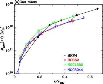
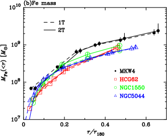
Figure 14: (a) Radial profiles of the integrated gas mass for MKW 4, HCG 62, the NGC 1550 group, and the NGC 5044 group. (b) Radial profiles of the integrated iron mass for MKW 4, HCG 62, the NGC 1550 group, and the NGC 5044 group. Dashed and solid lines correspond to the iron mass derived from the Fe abundances with the 1T and 2T model, respectively. The notations of colors and marks are the same as in figure 3.

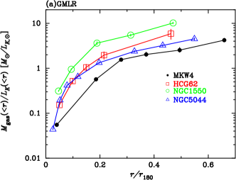
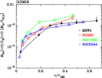
Figure 15: (a) Radial profiles of the integrated GMLRs with the $K$-band luminosity in units of $M_{\odot}/L_{\odot}$. The color and mark notations are the same as in figure 3. (b) Radial profiles of the integrated IMLRs with the $K$-band luminosity in units of $M_{\odot}/L_{\odot}$. The notations of color and mark are the same as in figure 3.

In order to derive gas mass profile, we calculated the electron density from the resultant normalizations with the 1T model because the spectra in the outer regions were well-represented with the 1T model. Figure 13 (a) shows radial profiles of the normalizations with the 1T model divided by the area, which corresponded to the surface brightness, for each group. We fitted the surface brightness profiles with a single $\beta$–model formula, $S(r)=S_{0}\left[1+\left(r/r_{\rm c}\right)^{2}\right]^{-3\beta+0.5}$. Here, $S_{0}$, $r_{c}$, and $\beta$ are the normalization, core radius, and index, respectively. Beyond $0.1~{}r_{180}$ of the NGC 1550 group, however, there is an discrepancy between the data and the best-fit single $\beta$–model. An power-law model well represented the data between 0.1 $r_{180}$ and 0.5 $r_{180}$. We, therefore, adopted the results of the power-law model fitting for the region outside 0.1 $r_{180}$. In figure 13 (a), for MKW 4, we also plotted the surface brightness profile derived from the previous ROSAT result (Sanderson et al., 2003), which were normalized to the brightness level observed with Suzaku by fitting with the fixed $\beta$ and $r_{c}$ to be 0.64 and 5.45^′, respectively. And then, we derived the electron density from the parameters by fitting the surface brightness profile. The derived electron density profiles for each group were shown in figure 13 (b). We also plotted electron density profiles of MKW 4 derived from the previous ROSAT (Sanderson et al., 2003) and XMM (O’Sullivan et al., 2003) results in figure 13 (b). By integrating the electron density profiles, we derived the integrated gas mass profiles for each group. Figure 14 (a) shows the derived gas mass profile. For MKW 4, we used the gas mass derived from XMM (O’Sullivan et al., 2003) up to $0.2~{}r_{180}$, and, beyond $0.2~{}r_{180}$, we integrated the electron density derived from Suzaku observations. Note that, because MKW 4 has asymmetrical structure as mentioned in O’Sullivan et al. (2003), the gas mass profile for MKW 4 would have an uncertainty of a factor of 2. For the NGC 1550 group, we derived the deprojected electron density from the fitting result of normalizations up to $0.1~{}r_{180}$, and multiplied the volume of each rings to derive the integrated gas mass. Beyond $0.1~{}r_{180}$, we calculated the electron density profiles derived from power-law fitting from the normalizations per area with deprojection analysis. By integrating the electron density, we derived the integrated gas mass beyond $0.1~{}r_{180}$

In figure 14 (b), we derived the integrated iron mass profiles from the gas mass from the resultant normalizations with the 1T model and the Fe abundances derived from the 1T and 2T model fits with the ATOMDB version 2.0.1. The radial iron mass profiles with the 2T model for each group were higher by $\sim 20\%$ at the most than those with the 1T model. The difference of Fe mass between the 1T and 2T model reflects the multiphase ICM in the center of groups and the consequent Fe-bias (e.g. Buote 2000; Buote et al. 2003a, b; Johnson et al. 2011). The spectral fits with the version 1.3.1 gave higher Fe abundance by several tens of % than those with the version 2.0.1. The total iron mass, therefore, would have systematic uncertainties of several tens of % due to uncertainties of the temperature structure and the ATOMDB versions. We also calculated the integrated radial profile of GMLRs and IMLRs with the $K$-band luminosity as described in subsection 4.5, up to $\sim 0.5~{}r_{180}$ as shown in figure 15.

5 Discussion

We derived radial profiles of metal abundances in the ICM of the four groups of galaxies, MKW 4, HCG 62, the NGC 1550 group, and the NGC 5044 group, observed with Suzaku out to $\sim$ 0.5 $r_{180}$. In this section, we compare our results with those of clusters of galaxies observed with Suzaku and XMM, the Coma cluster ($kT\sim 7.8~{}{\rm keV}$, $z=0.023$, Matsushita et al. 2013b), the Perseus cluster ($kT\sim 6.1~{}{\rm keV}$, $z=0.018$, Matsushita et al. 2013a), the AWM 7 cluster ($kT\sim 3.5~{}{\rm keV}$, $z=0.017$, Sato et al. 2008), the Hydra A cluster ($kT\sim 3.0~{}{\rm keV}$, $z=0.054$, Sato et al. 2012), and the Abell 262 cluster ($kT\sim 2.0~{}{\rm keV}$, $z=0.016$, Sato et al. 2009b).

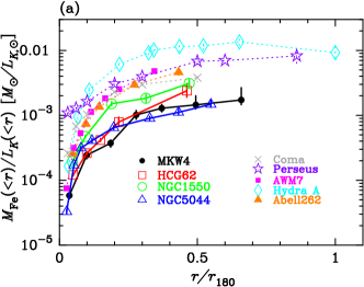
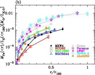
Figure 16: (a) Radial profiles of the integrated IMLRs, $M_{\rm Fe}(<r)/L_{K}(<r)$, in units of $M_{\odot}/L_{\odot}$ with the $K$-band luminosity for the Coma cluster (Matsushita et al., 2013b), the Perseus cluster (Matsushita et al., 2013a), the Centaurus cluster (Sakuma et al., 2011), the AWM 7 (Sato et al., 2008), Hydra A cluster (Sato et al., 2012), and the Abell 262 (Sato et al., 2009b),. (b) Radial profiles of the integrated IMLRs with total $K$-band luminosity within $r_{180}$, $M_{\rm Fe}(<r)/L_{K}(<r_{180})$.

If all galaxies synthesized a similar amount of metals per unit stellar mass, and groups and clusters of galaxies contain all the metals synthesized in the past, the IMLR values should be similar. Then, systems with lower gas mass would be expected to have higher ICM abundances. In subsection 5.1 and 5.2, we study the dependence of the IMLR and the Fe abundance on the system mass. The relative timing of metal enrichment and heating should affect on the present metal distributions in the ICM, and therefore, in subsection 5.3, we study the correlation of IMLR and entropy excess and discuss the early-metal enrichment in groups and clusters. The abundance ratios of Si/Fe and Mg/Fe in the ICM constrain the relative contributions from SNe Ia and SNecc, and in subsection 5.4 and 5.5, we compare these abundance ratios of the groups and clusters and nucleosynthesis models.

5.1 The dependence of the iron-mass-to-light ratios on the system scale

Figure 16 (a) compares the radial profiles of the integrated IMLR, $M_{\rm Fe}(<r)/L_{K}(<r)$, of the galaxy groups with those of several other clusters observed with Suzaku and XMM. Here, $M_{\rm Fe}(<r)$ and $L_{K}(<r)$ are integrated Fe mass and $K$-band luminosity within a radius $r$, respectively. The integrated IMLR of each cluster or group increases with radius out to 0.5 $r_{180}$, and beyond the radius, those of the Hydra A cluster and the Perseus cluster become flatter. In other words, the distribution of Fe in the ICM are much more extended than the stellar distribution at least out to 0.5 $r_{180}$. Outside the core of galaxy groups, if metal enrichment occurs after the formation of clusters, the metal distribution would be expected to follow the stellar distribution. Because of the limited spatial resolution of Suzaku, the core of galaxy groups, where are filled the newly formed metals spread out by the AGN action, did not discuss here. Therefore, the increase of IMLR with radius indicates that a significant fraction of Fe synthesized in an early phase of cluster evolution.

As shown in figure 16 (a), the IMLR of the groups were significantly smaller than those of the other clusters at a given radius in units of $r_{180}$. Since the IMLR profiles increase with radius, comparison of the total IMLR values requires observations of IMLR profiles out to the virial radii. However, if we extrapolate the observed IMLR profiles of groups out to the virial radii, it may be difficult to reach the level of clusters.

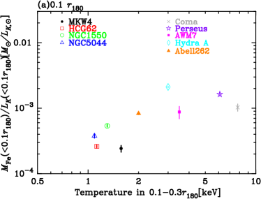
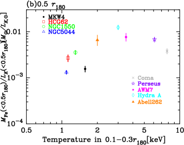
Figure 17: Integrated IMLRs within $\sim 0.1~{}r_{180}$ (a) and $\sim 0.5~{}r_{180}$ (b) as a function of the ICM temperature at 0.1–0.3 $r_{180}$ of galaxy groups compared with the Coma cluster (Matsushita et al., 2013b), the Perseus cluster (Matsushita et al., 2013a), the Centaurus cluster (Sakuma et al., 2011), the AWM 7 (Sato et al., 2008), Hydra A cluster (Sato et al., 2012), and the Abell 262 (Sato et al., 2009b).

To derive the three dimensional $K$-band luminosity profiles, we deprojected the radial luminosity profiles in the $K$-band assuming a spherical symmetry. However, the luminosity distribution of galaxies in each cluster was far from the spherical symmetry, especially for luminous galaxies. As a result, several luminous galaxies could cause artificial breaks in the luminosity profiles, especially for poor systems with a smaller number of galaxies. Therefore, in figure 16 (b), we also show the ratio of integrated iron mass, $M_{\rm Fe}(<r)$, to the total $K$-band luminosity within $r_{180}$, $M_{\rm Fe}(<r)/L_{K}(<r_{180})$, to study the difference in the IMLR between groups and clusters. Here, the total $K$-band luminosities of the other groups and clusters were calculated in the same way with our sample groups from the 2MASS catalogue. Then, $M_{\rm Fe}(<r)/L_{K}(<r_{180})$ of groups are also systematically lower than those in clusters. The derived profiles of $M_{\rm Fe}(<r)/L_{K}(<r_{180})$ became smoother than those of $M_{\rm Fe}(<r)/L_{K}(<r)$, that are reflecting smooth iron density profiles. The radial profiles of $M_{\rm Fe}(<0.5~{}r_{180})/L_{K}(<r_{180})$ of the Hydra A cluster and the Perseus cluster agree very well, although those of $M_{\rm Fe}(<r)/L_{K}(<r)$ have a discrepancy of a factor of 2–3 at a given radius in units of $r_{180}$. Because of the higher redshift of the Hydra A cluster and the lower ICM temperature, the number of galaxies detected in Hydra A with 2MASS might not be sufficient to deprojected the luminosity profiles in the $K$-band. However, at $\sim r_{180}$, the systematic uncertainties due to the limited number of galaxies are relatively small.

In this paper, we use the scaling radius, $r_{180}$, using the average ICM temperature, $\left<kT\right>$, expected from numerical simulations. However, non-gravitational energy inputs in the past may change the $r_{180}$–$\left<kT\right>$ relation. The $r_{500}$–$\left<kT\right>$ relation estimated for groups by Finoguenov et al. (2006, 2007) and that used for clusters by Pratt et al. (2009) differ by $\sim$ 20% at average ICM temperature of 1 keV. This uncertainty is even smaller than the radial range in a annular region used in our analysis. If there is a systematic uncertainty in the scaling radius of 20%, Figure 16 shows that the systematic uncertainties in the IMLR values at 0.5 $r_{180}$ are about 10–30%, which are much smaller than the variation in the IMLR.

To study the dependence of the IMLR on the average ICM temperature, in figure 17, we plotted the integrated IMLRs of the galaxy groups and clusters at $\sim 0.1~{}r_{180}$ and $\sim 0.5~{}r_{180}$ with $K$-band, $M_{\rm Fe}(<0.1~{}r_{180})/L_{K}(<0.1~{}r_{180})$ and $M_{\rm Fe}(<0.5~{}r_{180})/L_{K}(<0.5~{}r_{180})$, against the ICM temperature at 0.1–0.3 $r_{180}$. At $\sim 0.1~{}r_{180}$ and $\sim 0.5~{}r_{180}$, systems with smaller IMLR values have relatively lower ICM temperatures, although there is a significant scatter in the IMLR below 2 keV. The NGC 5044 group and MKW 4 show the smallest $M_{\rm Fe}(<0.5~{}r_{180})/L_{K}(<0.5~{}r_{180})$ values, which are an order of magnitude smaller than those of rich clusters.

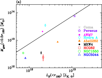
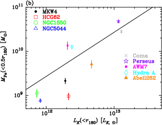
Figure 18: (a) The integrated gas mass within $0.5~{}r_{180}$, $M_{\rm gas}(<0.5~{}r_{180})$, is plotted against the integrated $K$-band luminosity within $r_{180}$, $L_{K}(<r_{180})$. The color and mark notations are the same as figure 17. The solid line corresponds to a constant $M_{\rm gas}(<0.5~{}r_{180})$ to $L_{K}(<r_{180})$ ratio of 7.39 $M_{\odot}/L_{\odot}$ , which is averaged for the Coma cluster, the Perseus cluster, and the AWM 7. (b) The integrated iron mass, $0.5~{}r_{180}$, $M_{\rm Fe}(<0.5~{}r_{180})$, is plotted against $L_{K}(<r_{180})$. The solid line corresponds to a constant $M_{\rm Fe}(<0.5~{}r_{180})$ to $L_{K}(<r_{180})$ ratio of $2.7\times 10^{-3}M_{\odot}/L_{\odot}$ , which is averaged for the Coma cluster, the Perseus cluster, and the AWM 7.

In figure 18(a), we plotted integrated gas mass out to $0.5~{}r_{180}$, $M_{\rm gas}(<0.5~{}r_{180})$, of the four groups of galaxies in our sample with those of the other clusters as a function of $L_{K}(<r_{180})$. $M_{\rm gas}(<0.5~{}r_{180})$ of these clusters of galaxies and the NGC 1550 group are mostly proportional to $L_{K}(<r_{180})$. In contrast, the other groups and Abell 262 cluster have smaller $M_{\rm gas}(<0.5~{}r_{180})$ to $L_{K}(<r_{180})$ ratio by a factor of $\sim$ 5. The right panel of figure 18 shows the integrated Fe mass out to $0.5~{}r_{180}$, $M_{\rm Fe}(<0.5~{}r_{180})$, against $L_{K}(<r_{180})$. The groups with lower $M_{\rm gas}(<0.5~{}r_{180})$ for a given $L_{K}(<r_{180})$ have lower $M_{\rm Fe}(<0.5~{}r_{180})$ values.

In summary, some groups of galaxies have lower gas-mass-to-light ratios with lower IMLR values. If all galaxies synthesized a similar amount of metals per unit stellar mass, the observed lower IMLR values indicate that a significant fraction of Fe synthesized in the past is not located within 0.5 $r_{180}$ of these groups of galaxies.

5.2 The dependence on the Fe abundance on the system scale

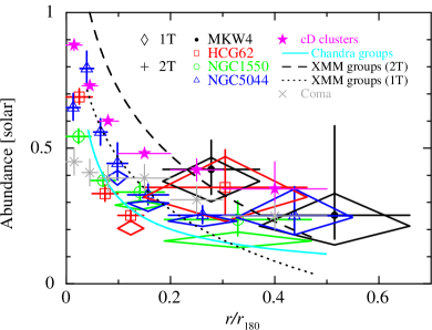
Figure 19: Radial profiles of the Fe abundance derived from the 2T model (crosses) with the ATOMDB version 2.0.1. We also plotted the Fe abundance profiles with the 1T model (diamonds) beyond $0.1~{}r_{180}$ with the ATOMDB version 2.0.1. The notations of colors and symbols are the same as in figure 4. The weighted average Fe abundance of relaxed clusters with a cD galaxy at their center observed with XMM (Matsushita, 2011) are shown by filled stars (magenta). The best-fit regression relation for groups observed with Chandra (Rasmussen & Ponman, 2007) is indicated by the solid (cyan) line, and those for cool core groups with XMM (2T: dashed line, 1T: dotted line, Johnson et al. 2011) are also plotted. Here, we corrected the XMM and Chandra results for the differences of the definition on the solar abundance table and the virial radius.

The radial profiles of the Fe abundance of the galaxy groups with previous measurements for clusters of galaxies are shown in figure 19. Absolute values of the Fe abundance derived from the Fe-L spectral fitting could have larger systematic uncertainties than the IMLR, considering that a higher Fe abundance gives a lower normalization. The 2T model fits on the Fe-L spectra sometimes give significantly higher Fe abundances than the 1T model fits by several tens of percents (Buote, 2000; Johnson et al., 2011; Murakami et al., 2011). As shown in subsection 4.2, using the 2T model fits, the new version of ATOMDB yielded lower Fe abundances than the old one, especially at the group center.

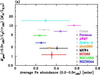
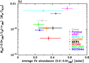
Figure 20: (a)The $M_{gas}(<0.5~{}r_{180})$ to $L_{K}(<r_{180})$ ratio as a function of the average Fe abundances in 0.2–0.5 $r_{180}$ for galaxy groups compared with the Coma cluster (Matsushita et al., 2013b), the Perseus cluster (Matsushita et al., 2013a), the AWM 7 (Sato et al., 2008), Hydra A cluster (Sato et al., 2012), and the Abell 262 (Sato et al., 2009b). Here, the result of the AWM 7 cluster is an extrapolation from the results within $\sim 0.4~{}r_{180}$. (b)The same as (a), but Fe mass, $M_{Fe}(<0.5~{}r_{180})$.

Beyond $0.1~{}r_{180}$, the Fe abundances of our sample groups derived from the 1T and 2T model fits are about 0.2–0.4 solar, except for the 1T model result for the NGC 1550 group. Beyond $0.1~{}r_{180}$, the Fe abundance profiles of the galaxy groups tend to be smaller than the weighted average of the nearby relaxed clusters with a cD galaxy at their center by several tens of percents, while agree well with that of the Coma cluster, which is one of the largest cluster in nearby Universe, observed with XMM (Matsushita, 2011). The Fe abundances of clusters were derived from the K$\alpha$ lines of Fe and as a result, systematic uncertainties should be smaller than those from the Fe-L lines. Even considering the systematic uncertainties in the derived Fe abundances from the Fe-L spectral fitting, the Fe abundances in the groups are not much higher than those of clusters.

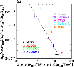
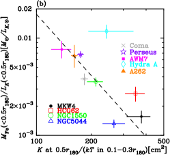
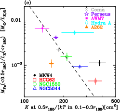
Figure 21: (a) The integrated IMLRs within $0.1~{}r_{180}$ as a function of the scaled entropy profiles at $\sim 0.1~{}r_{180}$. The dashed lines indicate the best–fit power-law model. (b)The same as (a), but at 0.4–0.5 $r_{180}$. (c) The $M_{\rm Fe}(<0.5~{}r_{180})$ to $L_{K}(<r_{180})$ ratios against scaled entropy at 0.4–0.5 $r_{180}$. The color and mark notations are the same as figure 16.

Beyond $0.1~{}r_{180}$, our Fe abundances derived from the 2T model tend to be lower and flatter than the best-fit regression relation from the 2T model fits on the results of the groups observed with XMM (Johnson et al., 2011) and higher than the relation of the 1T model fits on Chandra data (Rasmussen & Ponman, 2007). Some part of this difference may be caused by an difference in the adopted atomic data, since the previous results were derived using the old version of ATOMDB. The differences in the sample may also cause the discrepancy, since our sample is limited within relatively X-ray luminous groups.

The observed dependency of stellar to gas mass ratios within $r_{500}$ on the total system mass has been sometimes interpreted that star formation efficiency from baryons also depends on the system mass. Then, the Fe abundance in the ICM of systems with lower gas mass-to-light ratios is expected to be higher than those with higher values. In figure 20, $M_{\rm gas}(<0.5~{}r_{180})$/$L_{K}(<r_{180})$ and $M_{\rm Fe}(<0.5~{}r_{180})$/$L_{K}(<r_{180})$ are plotted against the Fe abundances at 0.2–0.5 $r_{180}$. There is no significant correlation between the Fe abundance and $M_{\rm gas}(<0.5~{}r_{180})$/$L_{K}(<r_{180})$ or $M_{\rm Fe}(<0.5~{}r_{180})$/$L_{K}(<r_{180})$. Among clusters of galaxies, the Fe abundance in 0.1–0.3 $r_{180}$ in the ICM does not depend on the ICM temperature (Matsushita, 2011), although the dependence of the stellar to gas mass ratio have been found among clusters.

5.3 Comparison of the entropy profiles with other systems

The difference in the ratio of gas-mass-to-stellar-mass would reflect differences in distributions of gas and stars, which in turn reflects the history of energy injection from galaxies to the ICM. If metal enrichment occurred before energy injection, the poor systems would carry relatively smaller metal mass with a smaller gas mass than rich clusters, whereas, the metal abundance would be quite similar to those in rich clusters.

Numerical simulations indicate that when clusters are radially scaled to the virial radius, or $r_{180}$, distribution of dark matter and baryons become self-similar(e.g. Navarro et al. 1995). Entropy carry important information about the thermal history of the ICM. Usually, the entropy parameter, $K$ is defined as,

$$K(r)=\frac{kT(r)}{n_{e}(r)^{2/3}},$$ (1)

where $kT(r)$ and $n_{e}(r)$ are temperature and deprojected electron density, respectively, at a radius $r$ from the cluster center. Especially, feedback from galaxies, such as galactic winds, changes ICM entropy rather than temperature. If there was no feedback, entropy profile is determined by pure gravitational heating. Then, at a given radius in units of $r_{180}$, the entropy, $K$, of the ICM is expected to be proportional to the average ICM temperature, $\left<kT\right>$ (Ponman et al., 1999, 2003). In other words, considering pure gravitational heating only, the scaled entropy, $K/\left<kT\right>$ is expected to be a constant. However, the relative entropy level in groups of galaxies is systematically higher than that for clusters of galaxies (Ponman et al., 1999, 2003), and the gas density profiles in the central regions of groups and poor clusters were observed to be shallower than those in the self-similar model (e.g. Cavagnolo et al. 2009).

In order to investigate the correction between entropy and IMLR profiles, we plotted IMLR profiles as a function of entropy profiles scaled by the ICM temperature in the 0.1–0.3 $r_{180}$. In figure 21 (a) , we plotted the IMLR within $0.1~{}r_{180}$ against the scaled entropy at $0.1~{}r_{180}$ . Figure 21 (b) is the same as (a), but the radius is changed to 0.5 $r_{180}$. Figure 21 (c) is plotted $M_{\rm Fe}(<0.5~{}r_{180})/L_{K}(<r_{180})$ as a function of the scaled entropy profiles at 0.4–0.5 $r_{180}$. We note that the ICM temperatures at this radial range of groups of galaxies are close to the average ICM temperature $\left<kT\right>$ (Rasmussen & Ponman, 2007). Excluding the Hydra A data, the IMLR correlate inversely well with the scaled entropy at each radius. When we plotted $M_{\rm Fe}(<0.5~{}r_{180})/L_{K}(<r_{180})$ against the scaled entropy at 0.5 $r_{180}$, the Hydra A data became closer to the relation of the other groups and clusters.

The increase of integrated IMLR with radius, the Fe abundance profiles, and the relationship between the scaled entropy and IMLR indicate early metal enrichments in clusters and groups of galaxies as already suggested by Matsushita (2011). If these systems synthesized Fe in an early phase of cluster evolution, the ICM is polluted in the same way. Then, the relative importance of the non-gravitational energy inputs in poor systems causes the difference in the gas distribution and as a result, the excess entropy inversely correlates with the integrated gas-mass-to-light ratio and IMLR. In systems with higher excess entropy, the gas is much more extended than stars, and as a result, the metals are also extended than stars.

5.4 Comparison of the Si/Fe and Mg/Fe ratios with other groups and clusters of galaxies

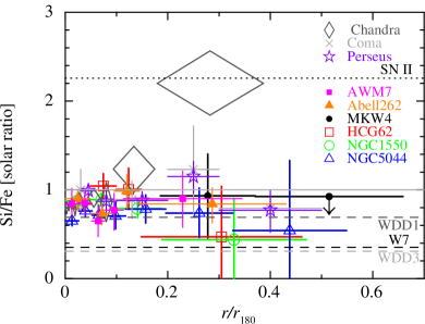
Figure 22: Radial profiles of the Si/Fe ratios derived from the 2T model fits with the ATOMDB version 2.0.1. The color and symbol notations are the same as in figure 4. The crosses, stars, filled squares, and filled triangles correspond to the Coma cluster (Matsushita et al., 2013b) the Perseus cluster (Matsushita et al., 2013a), AWM 7 (Sato et al., 2008), and Abell 262 cluster (Sato et al., 2009b), respectively. Diamonds show the radial profile of the weighted average of the Si/Fe ratio of groups observed with Chandra (Rasmussen & Ponman, 2007). Here, effects of differences in adopted solar abundance tables were corrected. Black, light gray, and dark gray dashed lines show the Si/Fe ratios of SN Ia yields of W7, WDD1, WDD3 model (Iwamoto et al., 1999), respectively. Black dotted line also shows the ratios of SNcc yields (Nomoto et al., 2006).

The ratios of $\alpha$-elements to Fe abundance give a strong constraint for the nucleosynthesis contribution from SNe Ia and SNecc. As shown in figure 22, the Si/Fe ratios in the ICM of the four galaxy groups in our sample are almost constant at $\sim 1$ solar ratio out to 0.2–0.3 $r_{180}$. Beyond 0.2–0.3 $r_{180}$ out to 0.5 $r_{180}$, the upper limit of the Si/Fe ratios are about unity in solar units. Here, we only plotted the Si/Fe ratios derived from the 2T model fits, since the 1T and 2T models gave almost the same values as shown in subsection 4.2. Figure 22 also shows the radial profiles of the Si/Fe ratios in the ICM of several clusters observed with Suzaku and XMM. The Si/Fe ratios in these clusters, the flat radial profiles at the solar ratio, agree well with those of our sample groups of galaxies. Although these previous measurements on abundance ratios were derived using the old ATOMDB except for the Perseus cluster, the systematic uncertainties in the Si/Fe ratios caused by the different version of ATOMDB may be relatively small as shown in subsection 4.2.

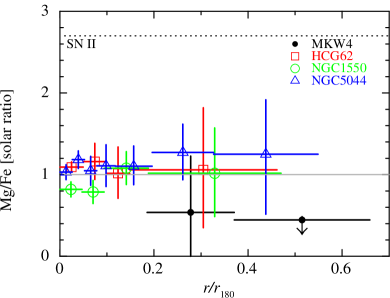
Figure 23: Radial profiles of the Mg/Fe ratios in the four groups derived from the 2T model with the ATOMDB version 2.0.1. The color and symbol notations are the same as in figure 4. Black dotted line shows the ratios of SNe II yields (Nomoto et al., 2006).

In figure 22, we also plotted the average Si/Fe ratios in the ICM of galaxy groups observed with Chandra (Rasmussen & Ponman, 2007). Within 0.1 $r_{180}$, the Si/Fe ratios of the groups and clusters observed with Suzaku agree well with the weighted average of groups observed with Chandra. However, beyond 0.2 $r_{180}$, the average Si/Fe ratio from the Chandra data is significantly higher than the Suzaku results. Some part of the difference in the Si/Fe ratio can be caused by the differences in the sample, since the Si/Fe ratios of the some X-ray luminous galaxy groups observed with Chandra are consistent with a flat radial profile. Especially, the Si/Fe ratios of three groups, the NGC 5044 group, HCG 62, and MKW 4, observed with Suzaku are consistent within error bars with those with Chandra, except for the outermost region ($\sim 0.2~{}r_{180}$) of the NGC 5044 group observed with Chandra.

Figure 23 shows the radial profiles of the Mg/Fe ratios of the four groups. As in the Si/Fe ratios, the Mg/Fe ratios are mostly consistent with the solar ratio and exhibit no significant radial dependence out to 0.5 $r_{180}$. The Mg/Fe ratios of other groups and poor clusters of galaxies at 0.1–0.3 $r_{180}$ with Suzaku using the old version of ATOMDB are mostly consistent with the solar ratio (Sato et al., 2008, 2009a, 2009b; Komiyama et al., 2009; Murakami et al., 2011; Sakuma et al., 2011). The systematic differences in the derived Mg/Fe ratios between the 1T and 2T model fits and between the two versions of ATOMDBs are smaller than a few tens of %. (subsection 4.1 and 4.2).

5.5 Contribution of SNe Ia and SNecc

The Si/Fe ratios of SNe Ia and SNecc yields from nucleosynthesis models are shown in figure 22. Here, SNecc yields by Nomoto et al. (2006) refer to an average over the Salpeter IMF of stellar masses from 10 to 50 $M_{\odot}$, with a progenitor metallicity of $Z=0.02$. The SNe Ia yields of the classical deflagration model, W7, and a delayed detonation (DD) models, WDD1, and WDD3, were taken from Iwamoto et al. (1999). The derived Si/Fe ratios were located between those of SNe Ia and SNecc yields. However, the systematic uncertainties in the Si/Fe ratio in SNe Ia nucleosynthesis models give an uncertainty in the relative contribution of both SN types as discussed in De Grandi & Molendi (2009). Because O and Mg are predominantly synthesized in SNecc, the O/Fe and Mg/Fe ratios give more unambiguous information on the relative contribution from SNecc and SNe Ia. The Mg/Fe ratio of SNecc yields assuming the Salpeter IMF with a progenitor metallicity of 0.02 is shown in figure 23. the Mg/Fe ratios of those groups are a factor of 2–3 smaller than that of the SNecc yields.

The number ratio of SNecc and SNe Ia to synthesize metals in the ICM was estimated with Suzaku and XMM data (e.g. de Plaa et al. 2007; Sato et al. 2007, 2008, 2010; Matsushita et al. 2013a, b). The observed abundance pattern of O, Mg, Si and Fe in the ICM observed with Suzaku is more consistent with a mixture of yields of SNecc with W7 or WDD3 models rather than that with the WDD1 model (Sato et al., 2007). The similarity of Mg/Si/Fe pattern of our sample with the previous Suzaku measurements also indicates a contribution of the W7 or WDD3 yields rather than WDD1 ones. The number ratio of SNecc and SNe Ia to synthesis the observed Mg, Si and Fe in the ICM of this work should close to the previous estimations, which are about 3–4 using SNe Ia yield of W7. Then, most of the Fe in the ICM should have been synthesized by SNe Ia.

The solar ratio of the Mg/Fe and Si/Fe ratios of our sample groups and those of clusters observed with Suzaku indicates that the contributions from two SN types to the metals in the ICM are universal. When systems are old enough, most SNe Ia and SNecc would have already exploded. To explain the abundance pattern of the stars in the solar neighborhood, the lifetimes of SNe Ia are confined within 0.5–3 Gyr, with a typical lifetime of 1.5 Gyr (Yoshii et al., 1996). Strolger et al. (2010) estimated a delay-time distribution for SNe Ia is about 3–4 Gyr and the observed SNe Ia rate in clusters of galaxies per unit stellar mass increases with redshift (e.g. Sand et al. 2012). In clusters of galaxies, to account for the Fe mass in the ICM, the past average rate of SNe Ia was much larger than the present rate of elliptical galaxies (e.g. Renzini et al. 1993; Matsushita et al. 2013a); accumulating the present SNe Ia rate over the Hubble time, the expected total Fe mass synthesized from SNe Ia in the past is an order of magnitude smaller than the observed total Fe mass out to the virial radius (Sato et al., 2012; Matsushita et al., 2013a). These results indicate that the lifetimes of most of SNe Ia are much shorter than the Hubble time. If stars in clusters have a similar initial mass function (IMF) with those of our Galaxy, the abundance pattern should naturally be similar to the solar abundance pattern.

6 Summary and Conclusions

We analyzed Suzaku data of the four galaxy group, MKW 4, HCG 62, the NGC 1550 group, and the NGC 5044 group out to 0.5 $r_{180}$. The temperature and metal abundance distributions were derived from the 1T and 2T model fits for the ICM with the ATOMDB version 1.3.1 and 2.0.1. The dependence on the temperature modeling and the versions of ATOMDB of these abundance ratios were relatively small. Beyond 0.1 $r_{180}$, the derived Fe abundance in the ICM was 0.2–0.4 solar, and consistent or slightly smaller than those of clusters of galaxies. The abundance ratios of Mg/Fe and Si/Fe of these groups and clusters are close to the solar ratio and exhibited no significant radial dependence. However, at 0.5 $r_{180}$, the integrated IMLR of some groups are systematically smaller than those of clusters of galaxies. The systems with smaller gas mass to light ratios have smaller IMLR values and the entropy excess is inversely correlated with the IMLR. These results indicate early metal enrichments in groups and clusters of galaxies.

Appendix A Estimations of the Galactic Foregrounds and Cosmic X-ray Background

It is important to estimate the Galactic and CXB emissions accurately, because the spectra, particularly in outer region of groups, suffer from the Galactic and CXB emissions strongly. We assumed the two Galactic emissions, the local hot bubble (LHB) and the Milky-Way halo (MWH), with a thermal plasma models (apec model; Smith et al. (2001)) as shown in Yoshino et al. (2009). The temperature of the LHB was fixed at 0.10 keV, while the normalization was a free parameter. We also allowed to vary the normalization and temperature of the MWH. The redshift and abundance were fixed at 0 and 1 solar, respectively, for the LHB and MWH components. We assumed the CXB component with a power-law model of a photon index, $\Gamma=1.4$. We simultaneously fitted the spectra for the outermost and other annuli regions with the following model formula; $constant~{}\times~{}(apec_{\rm LHB}~{}+~{}phabs~{}\times~{}(apec_{\rm MWH}~{}+$ $power{\rm-}law~{}+~{}vapec_{\rm ICM}~{}+~{}vapec_{\rm ICM}))$. Here, phabs model indicates the Galactic absorption. We assumed the 1T or 2T components for the ICM of the annular regions. Assumed two-temperature components for the ICM of the outermost region, these results did not change within systematic error compared with the results with the 1T model. The result of each simultaneous fits was consistent each other, and the weighted average results are shown in figure A.1.

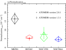
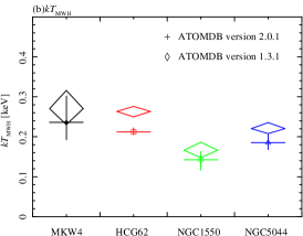
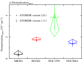
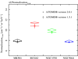
Figure A.1: Comparisons of the background component parameters, (a) LHB normalizations, (b) MWH temperature, (c) MWH normalizations, and (d) CXB normalizations. Normalization of the LHB and MWH (apec model) components divided by the solid angle, $\Omega^{U}$, assumed in the uniform-sky ARF calculation (20^′ radius), $Norm=\int n_{\rm e}n_{\rm H}dV\,/~{}\,[4\pi\,(1+z)^{2}D_{\rm A}^{~{}2}]\,/\,\Omega^{U}$ $\times 10^{-14}$ cm^-5 400$\pi$ arcmin^-2, where $D_{\rm A}$ is the angular distance to the source. On the other hand, normalization of the CXB (power-law) is units of photons cm² s^-1 sr^-1 keV^-1 at 1 keV.

With the ATOMDB version 2.0.1, the temperature of the MWH was 0.05 keV lower than that with the ATOMDB version 1.3.1, while the normalizations were consistent between the ATOMDB versions within statistical error ranges. The estimated background level with the version 1.3.1 were consistent with the typical values for the Galactic emissions (Yoshino et al., 2009).

Appendix B Figures of comparisons of the results with the ATOMDB versions

In this section, we summarize comparisons of the results by changing the ATOMDB versions. The reduced $\chi^{2}$ for the spectral fits for both the ATOMDB versions are shown figure B.1. We compared the temperatures and normalizations derived from the spectral fits with both of the ATOMDB versions in figure B.2. Figure B.3 and B.4 summarize comparisons of the abundance ratios of O, Mg, Si, and S to Fe for the 1T and 2T model fitting with both of the ATOMDB versions, in units of the solar ratios. The details of the results were addressed in subsection 4.2.

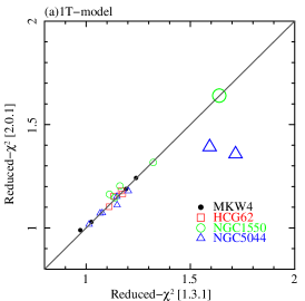
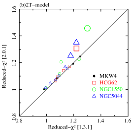
Figure B.1: Comparisons of the reduced $\chi^{2}$ for the spectral fits with the 1T (left) and 2T (right) models for both the ATOMDB versions. Note that the reduced $\chi^{2}$ in the innermost region for HCG 62 with the 1T model for the ATOMDB version 1.3.1 was higher than 3, thus, we did not plot in this figure. The notations are the same as in figure 3. Bigger marks indicate the $\chi^{2}$ within $0.05~{}r_{180}$.

Table B.1: Weighted averages of the abundance ratios in units of the solar ratios with ATOMDB version 1.3.1.

group	region	O/Fe [solar ratio]		Mg/Fe [solar ratio]		Si/Fe [solar ratio]		S/Fe [solar ratio]
		1T	2T	1T	2T	1T	2T	1T	2T
MKW 4	Alla	$1.34^{+2.35}_{-1.34}$	$1.48^{+2.53}_{-1.48}$	$0.13^{+0.56}_{-0.13}$	$0.24^{+0.77}_{-0.24}$	$0.75^{+0.67}_{-0.68}$	$0.67^{+0.66}_{-0.63}$	$1.19^{+1.18}_{-1.14}$	$1.08^{+1.15}_{-1.08}$
HCG 62	$<0.1~{}r_{180}$	$0.77^{+0.16}_{-0.16}$	$0.58^{+0.09}_{-0.09}$	$0.72^{+0.08}_{-0.08}$	$0.91^{+0.07}_{-0.07}$	$0.87^{+0.08}_{-0.08}$	$0.80^{+0.06}_{-0.06}$	$1.94^{+0.20}_{-0.20}$	$0.97^{+0.10}_{-0.10}$
	$>0.1~{}r_{180}$	$1.34^{+0.72}_{-0.72}$	$0.96^{+0.41}_{-0.41}$	$0.62^{+0.45}_{-0.46}$	$0.85^{+0.32}_{-0.33}$	$0.88^{+0.36}_{-0.34}$	$0.89^{+0.29}_{-0.29}$	$1.59^{+0.85}_{-0.83}$	$1.36^{+0.64}_{-0.65}$
	Alla	$0.80^{+0.16}_{-0.16}$	$0.60^{+0.09}_{-0.09}$	$0.72^{+0.08}_{-0.08}$	$0.91^{+0.07}_{-0.07}$	$0.87^{+0.08}_{-0.08}$	$0.81^{+0.06}_{-0.06}$	$1.92^{+0.19}_{-0.19}$	$0.98^{+0.10}_{-0.10}$
NGC 1550	$<0.1~{}r_{180}$	$0.78^{+0.29}_{-0.29}$	$0.79^{+0.27}_{-0.26}$	$0.56^{+0.11}_{-0.11}$	$0.73^{+0.11}_{-0.11}$	$0.80^{+0.05}_{-0.06}$	$0.79^{+0.05}_{-0.06}$	$0.95^{+0.08}_{-0.09}$	$0.82^{+0.08}_{-0.08}$
	$>0.1~{}r_{180}$	$0.23^{+0.74}_{-0.23}$	$0.53^{+0.78}_{-0.53}$	$0.80^{+0.29}_{-0.27}$	$0.98^{+0.27}_{-0.26}$	$0.72^{+0.16}_{-0.15}$	$0.72^{+0.15}_{-0.15}$	$0.93^{+0.25}_{-0.25}$	$0.84^{+0.25}_{-0.24}$
	Alla	$0.71^{+0.27}_{-0.25}$	$0.76^{+0.26}_{-0.24}$	$0.60^{+0.10}_{-0.11}$	$0.77^{+0.10}_{-0.10}$	$0.79^{+0.05}_{-0.06}$	$0.78^{+0.05}_{-0.05}$	$0.95^{+0.08}_{-0.08}$	$0.82^{+0.08}_{-0.07}$
NGC 5044	$<0.1~{}r_{180}$	$0.72^{+0.14}_{-0.13}$	$0.61^{+0.15}_{-0.14}$	$0.76^{+0.07}_{-0.06}$	$0.86^{+0.09}_{-0.08}$	$0.64^{+0.05}_{-0.05}$	$0.67^{+0.05}_{-0.05}$	$1.11^{+0.11}_{-0.10}$	$0.89^{+0.09}_{-0.09}$
	$>0.1~{}r_{180}$	$0.31^{+0.60}_{-0.31}$	$0.50^{+0.78}_{-0.13}$	$0.79^{+0.24}_{-0.24}$	$0.98^{+0.26}_{-0.25}$	$0.79^{+0.24}_{-0.24}$	$0.98^{+0.26}_{-0.25}$	$1.31^{+0.36}_{-0.37}$	$1.17^{+0.35}_{-0.34}$
	Alla	$0.73^{+0.13}_{-0.13}$	$0.61^{+0.15}_{-0.10}$	$0.76^{+0.06}_{-0.06}$	$0.88^{+0.08}_{-0.08}$	$0.65^{+0.05}_{-0.05}$	$0.68^{+0.05}_{-0.05}$	$1.13^{+0.10}_{-0.10}$	$0.91^{+0.09}_{-0.09}$

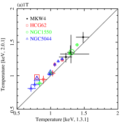
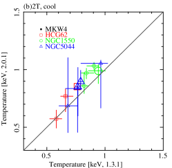
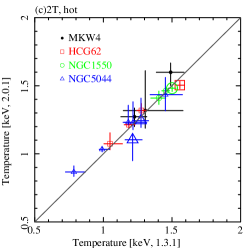
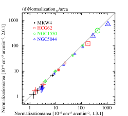
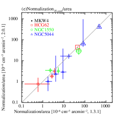
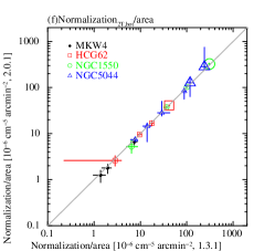
Figure B.2: Comparisons of the derived temperatures and normalizations with the ATOMDB version 1.3.1 and 2.0.1. (a)–(c): The comparisons of the temperatures from the 1T model fits, and the cooler and hotter component temperatures from the 2T model fits for the version 1.3.1 and 2.0.1. (d)–(f):The comparisons of the normalizations divided by the area from the 1T model fits, and the cooler and hotter component temperatures from the 2T model fits for the version 1.3.1 and 2.0.1. Bigger marks indicate the temperatures or normalizations within $0.05~{}r_{180}$.

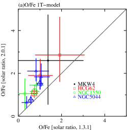
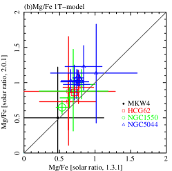
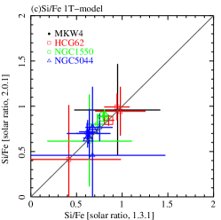
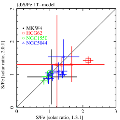
Figure B.3: Comparisons of (a) O/Fe, (b)Mg/Fe, (c) Si/Fe, and (d) S/Fe ratios derived from the 1T model fits with the ATOMDB version 1.3.1 and 2.0.1. The colors are the same as in figure 3. Bigger marks indicates the Fe abundance and the ratios within $0.05~{}r_{180}$.

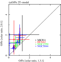
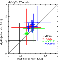
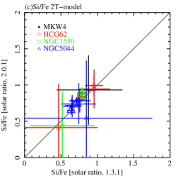
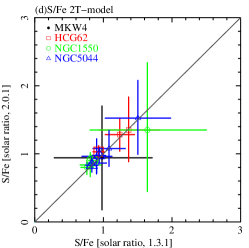
Figure B.4: The same as figure B.3 derived from 2T model.

References

- Buote (2000) Buote, D. A. 2000, ApJ, 539, 172
- Buote et al. (2003a) Buote, D. A., Lewis, A. D., Brighenti, F., & Mathews, W. G. 2003, ApJ, 594, 741
- Buote et al. (2003b) Buote, D. A., Lewis, A. D., Brighenti, F., & Mathews, W. G. 2003, ApJ, 595, 151
- Buote et al. (2004) Buote, D. A., Brighenti, F., & Mathews, W. G. 2004, ApJ, 607, L91
- Cavagnolo et al. (2009) Cavagnolo, K. W., Donahue, M., Voit, G. M., & Sun, M. 2009, ApJS, 182, 12
- Crook et al. (2007) Crook, A. C., Huchra, J. P., Martimbeau, N., Masters, K. L., Jarrett, T., & Macri, L. M. 2007, ApJ, 655, 790
- Crook et al. (2008) Crook, A. C., Huchra, J. P., Martimbeau, N., Masters, K. L., Jarrett, T., & Macri, L. M. 2008, ApJ, 685, 1320
- David et al. (1995) David, L. P., Jones, C., & Forman, W. 1995, ApJ, 445, 578
- De Grandi & Molendi (2009) De Grandi, S., & Molendi, S. 2009, A&A, 508, 565
- de Plaa et al. (2007) de Plaa, J., Werner, N., Bleeker, J. A. M., et al. 2007, A&A, 465, 345
- dell’Antonio et al. (1995) dell’Antonio, I. P., Geller, M. J., & Fabricant, D. G. 1995, AJ, 110, 502
- Evrard et al. (1996) Evrard, A. E., Metzler, C. A., & Navarro, J. F. 1996, ApJ, 469, 494
- Foster et al. (2010) Foster, A. R., Smith, R. K., Brickhouse, N. S., Kallman, T. R., & Witthoeft, M. C. 2010, Space Sci. Rev., 157, 135
- Finoguenov et al. (2006) Finoguenov, A., Davis, D. S., Zimer, M., & Mulchaey, J. S. 2006, ApJ, 646, 143
- Finoguenov et al. (2007) Finoguenov, A., Ponman, T. J., Osmond, J. P. F., & Zimer, M. 2007, MNRAS, 374, 737
- Giodini et al. (2009) Giodini, S., Pierini, D., Finoguenov, A., et al. 2009, ApJ, 703, 982
- Ishisaki et al. (2007) Ishisaki, Y., et al. 2007, PASJ, 59, 113
- Iwamoto et al. (1999) Iwamoto, K., Brachwitz, F., Nomoto, K., Kishimoto, N., Umeda, H., Hix, W. R., & Thielemann, F.-K. 1999, ApJS, 125, 439
- Johnson et al. (2011) Johnson, R., Finoguenov, A., Ponman, T. J., Rasmussen, J., & Sanderson, A. J. R. 2011, MNRAS, 413, 2467
- Kalberla et al. (2005) Kalberla, P. M. W., Burton, W. B., Hartmann, D., Arnal, E. M., Bajaja, E., Morras, R., Pöppel, W. G. L. 2005, A&A, 440, 775
- Kaastra, J. S. (1992) Kaastra, J. S.1992, An X-Ray Spectral Code for Optically Thin Plasmas (Internal SRON-Leiden Report, updated version 2.0)
- Kawaharada et al. (2003) Kawaharada, M., Makishima, K., Takahashi, I., et al. 2003, PASJ, 55, 573
- Kawaharada et al. (2009) Kawaharada, M., Makishima, K., Kitaguchi, T., et al. 2009, ApJ, 691, 971
- Komiyama et al. (2009) Komiyama, M., Sato, K., Nagino, R., Ohashi, T., & Matsushita, K. 2009, PASJ, 61, 337
- Koyama et al. (2007) Koyama, K., et al. 2007, PASJ, 59, 23
- Liedahl et al. (1995) Liedahl, D. A., Osterheld, A. L., & Goldstein, W. H. 1995, ApJ, 438, L115
- Lin et al. (2004) Lin, Y.-T., Mohr, J. J., & Stanford, S. A. 2004, ApJ, 610, 745
- Lodders (2003) Lodders, K. 2003, ApJ, 591, 1220
- Makishima et al. (2001) Makishima, K., et al. 2001, PASJ, 53, 401
- Markevitch et al. (1998) Markevitch, M., Forman, W. R., Sarazin, C. L., & Vikhlinin, A. 1998, ApJ, 503, 77
- Matsushita et al. (2007) Matsushita, K., Böhringer, H., Takahashi, I., & Ikebe, Y. 2007, A&A, 462, 953
- Matsushita (2011) Matsushita, K. 2011, A&A, 527, A134
- Matsushita et al. (2013a) Matsushita, K., Sakuma, E., Sasaki, T., Sato, K., & Simionescu, A. 2013, ApJ, 764, 147
- Matsushita et al. (2013b) Matsushita, K., Sato, T., Sakuma, E., & Sato, K. 2013, PASJ, 65, 10
- Mewe et al. (1985) Mewe, R., Gronenschild, E. H. B. M., & van den Oord, G. H. J. 1985, A&AS, 62, 197
- Mewe et al. (1986) Mewe, R., Lemen, J. R., & van den Oord, G. H. J. 1986, A&AS, 65, 511
- Morita et al. (2006) Morita, U., Ishisaki, Y., Yamasaki, N. Y., et al. 2006, PASJ, 58, 719
- Murakami et al. (2011) Murakami, H., et al. 2011, PASJ, 63, 963
- Nagino et al. (2009) Nagino, R., & Matsushita, K. 2009, A&A, 501, 157
- Navarro et al. (1995) Navarro, J. F., Frenk, C. S., & White, S. D. M. 1995, MNRAS, 275, 720
- Nomoto et al. (2006) Nomoto, K., Tominaga, N., Umeda, H., Kobayashi, C., & Maeda, K. 2006, Nuclear Physics A, 777, 424
- O’Sullivan et al. (2003) O’Sullivan, E., Vrtilek, J. M., Read, A. M., David, L. P., & Ponman, T. J. 2003, MNRAS, 346, 525
- Ponman et al. (1999) Ponman, T. J., Helsdon, S. F., & Finoguenov, A. 1999, Observational Cosmology: The Development of Galaxy Systems, 176, 64
- Ponman et al. (2003) Ponman, T. J., Sanderson, A. J. R., & Finoguenov, A. 2003, MNRAS, 343, 331
- Pratt et al. (2009) Pratt, G. W., Croston, J. H., Arnaud, M., Böhringer, H. 2009, A&A, 498, 361
- Rasmussen & Ponman (2007) Rasmussen, J., & Ponman, T. J. 2007, MNRAS, 380, 1554
- Rasmussen & Ponman (2009) Rasmussen, J., & Ponman, T. J. 2009, MNRAS, 399, 239
- Renzini et al. (1993) Renzini, A., Ciotti, L., D’Ercole, A., & Pellegrini, S. 1993, ApJ, 419, 52
- Sakuma et al. (2011) Sakuma, E., Ota, N., Sato, K., Sato, T., & Matsushita, K. 2011, PASJ, 63, 979
- Sand et al. (2012) Sand, D. J., Graham, M. L., Bildfell, C., et al. 2012, ApJ, 746, 163
- Sanderson et al. (2003) Sanderson, A. J. R., Ponman, T. J., Finoguenov, A., Lloyd-Davies, E. J., & Markevitch, M. 2003, MNRAS, 340, 989
- Sato et al. (2007) Sato, K., Yamasaki, N. Y., Ishida, M., et al. 2007, PASJ, 59, 299
- Sato et al. (2008) Sato, K., Matsushita, K., Ishisaki, Y., Yamasaki, N. Y., Ishida, M., Sasaki, S., & Ohashi, T. 2008, PASJ, 60, 333
- Sato et al. (2009a) Sato, K., Matsushita, K., Ishisaki, Y., Yamasaki, N. Y., Ishida, M., & Ohashi, T. 2009a, PASJ, 61, 353
- Sato et al. (2009b) Sato, K., Matsushita, K., & Gastaldello, F. 2009b, PASJ, 61, 365
- Sato et al. (2010) Sato, K., Kawaharada, M., Nakazawa, K., Matsushita, K., Ishisaki, Y., Yamasaki, N. Y., & Ohashi, T. 2010, PASJ, 62, 1445
- Sato et al. (2012) Sato, T., et al. 2012, PASJ, 64, 95
- Schlegel et al. (1998) Schlegel, D. J., Finkbeiner, D. P., & Davis, M. 1998, ApJ, 500, 525
- Smith et al. (2001) Smith, R. K., Brickhouse, N. S., Liedahl, D. A., & Raymond, J. C. 2001, ApJ, 556, L91
- Sun et al. (2003) Sun, M., Forman, W., Vikhlinin, A., et al. 2003, ApJ, 598, 250
- Sun et al. (2009) Sun, M., Voit, G. M., Donahue, M., et al. 2009, ApJ, 693, 1142
- Strolger et al. (2010) Strolger, L.-G., Dahlen, T., & Riess, A. G. 2010, ApJ, 713, 32
- Tokoi et al. (2008) Tokoi, K., et al. 2008, PASJ, 60, 317
- Yoshii et al. (1996) Yoshii, Y., Tsujimoto, T., & Nomoto, K. 1996, ApJ, 462, 266
- Urban et al. (2013) Urban, O., Simionescu, A., Werner, N., et al. 2013, arXiv:1307.3592
- Yoshino et al. (2009) Yoshino, T., et al. 2009, PASJ, 61, 805
- Zhang et al. (2011) Zhang, Y.-Y., Laganá, T. F., Pierini, D., et al. 2011, A&A, 535, A78