Crossing the Gribov horizon:
an unconventional study of geometric properties
of gauge-configuration space in Landau gauge

Abstract:

We prove a lower bound for the smallest nonzero eigenvalue of the Landau-gauge Faddeev-Popov matrix in Yang-Mills theories. The bound is written in terms of the smallest nonzero momentum on the lattice and of a parameter characterizing the geometry of the first Gribov region. This allows a simple and intuitive description of the infinite-volume limit in the ghost sector. In particular, we show how nonperturbative effects may be quantified by the rate at which typical thermalized and gauge-fixed configurations approach the Gribov horizon. Our analytic results are verified numerically in the SU(2) case through an informal, free and easy, approach. This analysis provides the first concrete explanation of why the so-called scaling solution of the Dyson-Schwinger equations is not observed in lattice studies.

1 Infinite-Volume Limit and the Boundary of the First Gribov Region $\Omega$

Since the original work by Gribov [1], innumerous numerical and analytic studies (see, for example, the reviews [2, 3]) have focused on the infrared (IR) behavior of Yang-Mills Green’s functions in minimal-Landau gauge and on its connection to color confinement [4]. On the lattice, a detailed description of the IR sector of Yang-Mills theories requires an extrapolation to infinite volume. In minimal-Landau gauge, this extrapolation should be governed by a (widely accepted) axiom stating that

At very large volumes, the functional integration gets concentrated on the boundary $\partial\Omega$ of the first Gribov region $\Omega$ [defined by transverse gauge configurations with all nonnegative eigenvalues of the Faddeev-Popov (FP) matrix ${\cal M}$].

Thus, the functional integration should be strongly dominated at very large volumes by configurations belonging to a thin layer close to $\partial\Omega$, i.e. typical configurations should be characterized by very small values for the smallest nonzero eigenvalue $\lambda_{1}$ of ${\cal M}$. Indeed, numerical studies show that $\lambda_{1}$ goes to zero as the lattice volume increases.

In Ref. [5] we have introduced the following inequalities for the ghost propagator $G(p)$ in momentum space

$$\frac{1}{N_{c}^{2}-1}\,\frac{1}{\lambda_{1}}\,\sum_{b}\,|{\widetilde{\psi}_{1}(b,p)}|^{2}\;\leq\;G(p)\;\leq\;\frac{1}{\lambda_{1}}\;,$$ (1)

where ${\widetilde{\psi}_{1}(b,p)}$ is the (Fourier-transformed) eigenvector of the FP matrix ${\cal M}$ corresponding to the eigenvalue $\lambda_{1}$ and $b=1,2,\ldots,N_{c}^{2}-1$ is a color index running over the $N_{c}^{2}-1$ generators of the SU($N_{c}$) gauge group. Note that, on the lattice and for large lattice volumes, the smallest nonzero momentum $p_{min}$ is of the order of $1/L$, where $L$ is the lattice size. Thus, if $\lambda_{1}$ behaves as $\,L^{-2-\alpha}\,$ in the infinite-volume limit, the inequality $\alpha>0$ is a necessary condition to obtain an IR-enhanced ghost propagator $G(p_{min})\sim 1/p_{min}^{2+2\kappa}$ (with $\kappa>0$), as predicted in the Gribov-Zwanziger confinement scenario [3] and by the scaling solution [6] of the Dyson-Schwinger equations (DSEs) for gluon and ghost propagators. At the same time, if the quantity $\,|{\widetilde{\psi}_{1}(b,p_{min})}|^{2}\,$ behaves as $L^{-\gamma}$ at large $L$, the inequality $\alpha-\gamma>0$ is a sufficient condition to have $\kappa>0$. Therefore, in order to describe the extrapolation to infinite volume in the ghost sector, we can re-formulate the above axiom and say that

The key point seems to be the rate at which $\lambda_{1}$ goes to zero, which, in turn, should be related to the rate at which a thermalized and gauge-fixed configuration approaches $\partial\Omega$.

This is, however, just a qualitative statement. Indeed, in order to make the above axiom quantitative, we need to relate the eigenvalue $\lambda_{1}$ to the geometry of the Gribov region $\Omega\,$. A first step in this direction was taken in Ref. [7]. There, we proved a lower bound for $\lambda_{1}$ [see Eq. (10) below] that relates this eigenvalue to the distance of the gauge configuration $A\in\Omega$ from the boundary $\partial\Omega$. As a consequence, we were able to provide the first concrete explanation of why the scaling solution of the DSEs is not observed in lattice studies. The main results of Ref. [7] are presented below.

2 Lower bound for $\lambda_{1}$

The (lattice) Landau gauge is usually imposed by minimizing the functional

$${\cal E}[U;\omega]\,=\,-Tr\,\sum_{x,\mu}\,\omega(x)\;U_{\mu}(x)\;\omega^{\dagger}(x+a\,e_{\mu})$$ (2)

with respect to the lattice gauge transformations $\,\omega(x)\in$ SU($N_{c}$). This defines the first Gribov region

$$\Omega\,\equiv\,\left\{\,U:\,\partial\cdot A=0\mbox{,}\;\quad{\cal M}\,=\,-D\cdot\partial\,\geq\,0\,\right\}\;,$$ (3)

where $D^{bc}(x,y)[A]$ is the covariant derivative and ${\cal M}(b,x;c,y)[A]$ is the FP matrix. One can show [8] that all gauge orbits intersect $\Omega$ and that this region is characterized by the following three properties [9] (see also [3, 7]): 1) the trivial vacuum $A_{\mu}=0$ belongs to $\Omega$; 2) the region $\Omega$ is convex; 3) the region $\Omega$ is bounded in every direction.

From the definition of ${\cal M}[A]$ [see Eq. (3)] it is clear that the FP matrix has a trivial null eigenvalue, corresponding to constant vectors. Then, if we indicate with $\lambda_{1}\left[\,{\cal M}[A]\,\right]$ the smallest nonzero eigenvalue of ${\cal M}[A]$, we can introduce the definition

$$\lambda_{1}\left[\,{\cal M}[A]\,\right]\,=\,\min_{\chi}\,\left(\chi\,,\left[\,{\cal M}[A]\,\right]\,\chi\right)\;,$$ (4)

where $\chi$ are non-constant vectors such that $(\chi\,,\chi)=1$. Also, by noticing that the operators $D[A]$, ${\cal M}[A]=-\partial^{2}+{\cal K}[A]$ and ${\cal K}[A]$ are linear in the gauge field $A$, one can write

$${\cal M}[\rho A]\,=\,-\partial^{2}+{\cal K}[\rho A]\,=\,(1-\rho)\,(-\partial^{2})\,+\,\rho\,{\cal M}[A]\;.$$ (5)

At the same time, for $A\in\Omega$, $\rho\in[0,1]$ and using the first and second properties above, we have that $\rho A\in\Omega$. This result applies in particular to configurations $A^{\prime}$ belonging to the boundary $\partial\Omega$ of $\Omega$. Thus, by using the definition (4), Eq. (5) in the case $A^{\prime}\in\partial\Omega$ and the concavity of the minimum function [10], i.e. $\,\min_{\chi}\left(\chi,\left[M_{1}+M_{2}\right]\chi\right)\,\geq\,\min_{\chi}\left(\chi,M_{1}\chi\right)+\min_{\chi}\left(\chi,M_{2}\chi\right)\,$ (where $M_{1}$and $M_{2}$ are two generic square matrices), we obtain [7]

$$\lambda_{1}\left[\,{\cal M}[\rho A^{\prime}]\,\right] = \lambda_{1}\left[(1-\rho)\,(-\partial^{2})\,+\,\rho\,{\cal M}[A^{\prime}]\right]$$ (6)

$$= \min_{\chi}\,\left(\chi\,,\left[\,(1-\rho)\,(-\partial^{2})\,+\,\rho\,{\cal M}[A^{\prime}]\,\right]\,\chi\right)$$ (7)

$$\geq (1-\rho)\min_{\chi}\left(\chi,(-\partial^{2})\,\chi\right)\,+\,\rho\min_{\chi}\,\left(\chi\,,{\cal M}[A^{\prime}]\,\chi\right)\;.$$ (8)

Since $A^{\prime}\in\partial\Omega$, i.e. the smallest non-trivial eigenvalue of the FP matrix ${\cal M}[A^{\prime}]$ is null, and since the smallest non-trivial eigenvalue of (minus) the Laplacian $-\partial^{2}$ is $p^{2}_{min}$, we find

$$\lambda_{1}\left[\,{\cal M}[\rho A^{\prime}]\,\right]\,\geq\,(1-\rho)\,p^{2}_{min}\;.$$ (9)

Therefore, as the lattice size $L$ goes to infinity, the eigenvalue $\lambda_{1}\left[\,{\cal M}[\rho A^{\prime}]\,\right]$ cannot go to zero faster than $(1-\rho)\,p^{2}_{min}$. In particular, since $p^{2}_{min}\sim 1/L^{2}$ for large lattice size $L$, we have that $\lambda_{1}$ behaves as $\,L^{-2-\alpha}\,$ in the same limit, with $\alpha>0$, only if $1-\rho$ goes to zero at least as fast as $L^{-\alpha}$. Let us stress that this result applies to any Gribov copy belonging to $\Omega$.

With $\rho A^{\prime}=A$, the above inequality (9) may also be written as

$$\lambda_{1}\left[\,{\cal M}[A]\,\right]\;\geq\;[1-\rho]\,p^{2}_{min}\;.$$ (10)

Note that, in the Abelian case, one has ${\cal M}=-\partial^{2}$ and $\lambda_{1}=p^{2}_{min}$, i.e. non-Abelian effects are included in the factor $(1-\rho)$. At the same time, the quantity $1-\rho\leq 1$ measures the distance (see Ref. [7] for details) of a configuration $A\in\Omega$ from the boundary $\partial\Omega$ (in such a way that $A^{\prime}=\rho^{-1}A\in\partial\Omega$). Thus, the new bound (10) suggests all non-perturbative features of a minimal-Landau-gauge configuration $A\in\Omega$ to be related to its normalized distance $\rho$ from the “origin” $A=0$ [or, equivalently, to its normalized distance $1-\rho$ from the boundary $\partial\Omega$]. One should also stress that the above inequality becomes an equality if and only if the eigenvectors corresponding to the smallest nonzero eigenvalues of ${\cal M}[A]$ and $-\partial^{2}$ coincide.

As a consequence of the result (10), we can also find several new bounds. In particular, using the upper bound in Eq. (1) and the definition of the Gribov ghost form-factor $\sigma(p)$, we have

$$\frac{1}{p^{2}_{min}}\,\frac{1}{1-\sigma(p_{min})}\;\equiv\;G(p_{min})\;\leq\;\frac{1}{[1-\rho]\,p^{2}_{min}}$$ (11)

and therefore $\,\sigma(p_{min})\,\leq\,\rho$. This result is a stronger version of the so-called no-pole condition $\,\sigma(p)\,\leq\,1\,$ (for $p^{2}>0$), used to impose the restriction of the physical configuration space to the region $\Omega$. Similarly, for the horizon function $H$, defined in Eq. (3.10) of [12], one can prove that [7]

$$\frac{H}{dV(N_{c}^{2}-1)}\;\equiv\;h\;\leq\;\rho\;.$$ (12)

$N$	$\max(n)$	$\min(n)$	$\langle n\rangle$	$R_{\rm before}/1000$	$R_{\rm after}/1000$
16	30	6	17.2	15(3)	-30(12)
24	27	4	15.1	20(7)	-26(6)
32	19	5	11.7	26(9)	-51(20)
40	18	4	9.4	155(143)	-21(6)
48	13	2	7.8	21(5)	-21(5)
56	12	3	7.6	16(4)	-21(7)
64	11	2	6.8	20(7)	-42(18)
72	11	2	6.1	129(96)	-42(13)
80	12	3	6.1	15(4)	-24(4)

Table 1: The maximum, minimum and average number of steps $n$, necessary to “cross the Gribov horizon” along the direction $A_{\mu}^{b}(x)$, as a function of the lattice size $N$. We also show the ratio $R$ [see Eq. (13)], divided by 1000, for the modified gauge fields ${\widehat{A}}_{\mu}^{(n-1)}(x)=\tau_{n-1}\;A_{\mu}(x)$ and ${\widehat{A}}_{\mu}^{(n)}(x)=\tau_{n}\;A_{\mu}(x)$, i.e. for the configurations immediately before and after crossing $\partial\Omega$.

3 Simulating the Math

In order to verify the new bounds presented in the previous section, we started by considering the third property of the region $\Omega$, i.e. the fact that $\Omega$ is bounded in every direction. To this end we “simulate” the mathematical proof of this property, i.e. given a thermalized gauge configuration $A_{\mu}(x)$, we apply the scale transformations $\,{\widehat{A}}_{\mu}^{(i)}(x)\,=\,\tau_{i}\;A_{\mu}(x)\,$ such that: a) $\tau_{0}=1$, b) $\tau_{i}=\delta\,\tau_{i-1}$, c) $\delta=1.001$ if $\lambda_{1}\geq 5\,\times\,10^{-3}$, d) $\delta=1.0005$ if $\lambda_{1}\in[5\,\times\,10^{-4},\,5\,\times\,10^{-3})$ and e) $\delta=1.0001$ if $\lambda_{1}<5\,\times\,10^{-4}$, with $\lambda_{1}$ evaluated at the step $i-1$. Clearly, after $n$ steps, the modified gauge field ${\widehat{A}}_{\mu}^{(n)}(x)$ does not belong to the region $\Omega$ anymore, i.e. the eigenvalue $\lambda_{1}$ of ${\cal M}[{\widehat{A}}^{(n)}]$ is negative (while the eigenvalue $\lambda_{2}$ is still positive). Results for the number of steps $n$ necessary to “cross the Gribov horizon” along the direction $A_{\mu}^{b}(x)$ are reported in Table 1. It is interesting to note that the value of $n$ decreases as the lattice side $N$ increases, i.e. configurations with larger physical volume are (on average) closer to the boundary $\partial\Omega$.

In the same table we also show the value of the ratio

$$R\,=\,\frac{({\cal E}^{\prime\prime\prime})^{2}}{\lambda_{1}\,{\cal E}^{\prime\prime\prime\prime}}$$ (13)

for the rescaled gauge fields ${\widehat{A}}_{\mu}^{(n-1)}(x)=\tau_{n-1}\;A_{\mu}(x)$ and ${\widehat{A}}_{\mu}^{(n)}(x)=\tau_{n}\;A_{\mu}(x)$, i.e. for the configurations immediately before and after crossing the first Gribov horizon $\partial\Omega$. The same ratio is also shown in Fig. 1 (left plot), as a function of the iteration step $i$, for a typical configuration and for the lattice volume $V=16^{4}$. For the same configuration we also show (see Fig. 1, right plot) the dependence of $\lambda_{2}$, $|{\cal E}^{\prime\prime\prime}\,|$ and of ${\cal E}^{\prime\prime\prime\prime}\,$ on the iteration step $i$. One clearly sees that these quantities have a slow and continuous dependence on the factors $\tau_{i}$. On the other hand, since $\lambda_{1}$ decreases as $\tau_{i}$ increases, we find that the ratio $R$ usually increases with $\tau_{i}$ and that $R_{n-1}\approx-R_{n}$, due to the change in sign of $\lambda_{1}$ as the first Gribov horizon is crossed (see the fourth and the fifth columns in Table 1 and the left plot in Fig. 1). At the same time one can check (see the right plot in Figure 1) that the second smallest (non-trivial) eigenvalue $\lambda_{2}$ stays positive, i.e. the final configuration ${\widehat{A}}_{\mu}^{(n)}(x)=\tau_{n}\;A_{\mu}(x)$ belongs to the second Gribov region [1, 12].

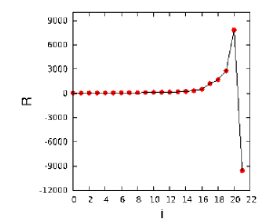
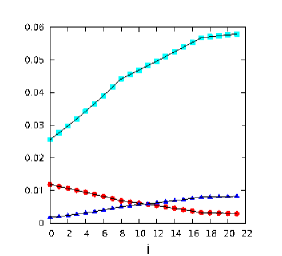
Figure 1: Left: plot of the ratio $R$ [see Eq. (13)], as a function of the iteration step $i$, for a typical configuration and lattice volume $V=16^{4}$. Right: plot of $\lambda_{2}$ (redfull circes), $|{\cal E}^{\prime\prime\prime}\,|$ (cyanfull squares) and ${\cal E}^{\prime\prime\prime\prime}\,$ (bluefull triangles) as a function of the iteration step $i$, for the same configuration considered in the left plot.

Once we have found a configuration ${\widehat{A}}_{\mu}^{(n)}\notin\Omega$, we can use the definition

$$A_{\mu}^{\prime}(x)\,=\,\frac{{\widehat{A}}_{\mu}^{(n-1)}(x)+{\widehat{A}}_{\mu}^{(n)}(x)}{2}\,=\,\frac{\tau_{n-1}+\tau_{n}}{2}\,A_{\mu}(x)\,\equiv\,{\widetilde{\tau}}\,A_{\mu}(x)$$ (14)

as a candidate for a configuration belonging to the boundary $\partial\Omega$. This gives us an estimate for the parameter $\rho=1/{\widetilde{\tau}}<1$ and allows us to test the inequalities presented in the previous Section. The numerical data tell us that most lattice configurations $A$ are very close to the first Gribov horizon $\partial\Omega$, i.e. one usually finds $\rho\approx 1$ (see Figure 2, left plot). Moreover, the quantity $1-\rho$ goes to zero reasonably fast. On the other hand, the inequality (10) is far from being saturated by the lattice data (see Figure 2, right plot), and the situation seems to become worst in the infinite-volume limit. The same observation applies (see Fig. 2, right plot) to the lower bound in Eq. (1). Finally, for large lattice size $L$ one finds $\,G(p_{min})\,\mathrel{\hbox to0.0pt{\lower 3.0pt\hbox{$\mathchar 536\relax$}\hss}\raise 2.0pt\hbox{$\mathchar 316\relax$}}\,1/\lambda_{1}\,$ (see again Figure 2, right plot). These results are all consistent with the fact that the eigenvector $\psi_{1}$ is very different from the plane waves corresponding to $p^{2}_{min}$, which clarifies why the ghost propagator $G(p)$ is not enhanced in the IR limit. Conversely, configurations producing an IR-enhanced ghost propagator should almost saturate the new bound (10), i.e. their eigenvector $\psi_{1}$ should have a large projection on at least one of the plane waves corresponding to $p^{2}_{min}$. Thus, in the scaling solution [6], nonperturbative effects, such as color confinement, should be driven by configurations whose FP matrix ${\cal M}$ is “dominated” by an eigenvector $\psi_{1}$ very similar to the corresponding eigenvector of ${\cal M}=-\partial^{2}\,$, i.e. to the eigenvector $\psi_{1}$ of the free case! This would constitute a very odd situation indeed. On the contrary, the massive solution of the DSEs of gluon and ghost propagators [16] is consistent with the more reasonable hypothesis that the eigenvector $\psi_{1}$ is in general very different from a free wave.

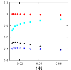
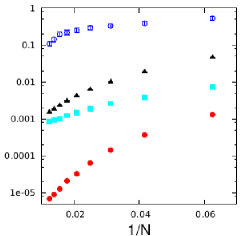
Figure 2: Left: plot of the (normalized) horizon function $h$ (blueempty circles), of the Gribov ghost form-factor $\sigma(p_{min})$ (full triangles), of the quantity $1-\lambda_{1}/p_{min}^{2}$ (cyanfull squares) and of their upper bound $\rho$ (redfull circles) as a function of the inverse lattice size $1/N$. Let us note that, in Ref. [15], it was proven that $\sigma(0)=h$ to all orders in the gauge coupling. Right: plot of the inverse of the lower bound in Eq. (1) (blueempty circles), of $1/G(p_{min})$ (full triangles), of $\lambda_{1}$ (cyanfull squares) and of the quantity $(1-\rho)\,p^{2}_{min}$ (redfull circles) as a function of the inverse lattice size $1/N$.

References

- [1] V. N. Gribov, Nucl. Phys. B 139 (1978) 1.
- [2] A. Cucchieri and T. Mendes, PoS QCD-TNT09 (2009) 026.
- [3] N. Vandersickel and D. Zwanziger, Phys. Rept. 520 (2012) 175.
- [4] J. Greensite, Acta Phys. Polon. B 40 (2009) 3355.
- [5] A. Cucchieri and T. Mendes, Phys. Rev. D 78 (2008) 094503.
- [6] L. von Smekal, A. Hauck and R. Alkofer, Annals Phys. 267 (1998) 1 [Erratum-ibid. 269 (1998) 182].
- [7] A. Cucchieri and T. Mendes, arXiv:1308.1283 [hep-lat], accepted for publication in Phys. Rev. D.
- [8] G. Dell’Antonio and D. Zwanziger, Commun. Math. Phys. 138 (1991) 291.
- [9] D. Zwanziger, Nucl. Phys. B 209 (1982) 336.
- [10] K. M. Abadir and and J. R. Magnus, Matrix Algebra, Cambridge University Press, New York, 2005.
- [11] A. Cucchieri, D. Dudal and N. Vandersickel, Phys. Rev. D 85 (2012) 085025.
- [12] D. Zwanziger, Nucl. Phys. B 378 (1992) 525.
- [13] A. Cucchieri, Nucl. Phys. B 521 (1998) 365.
- [14] D. Zwanziger, Nucl. Phys. B 412 (1994) 657.
- [15] M. A. L. Capri et al., Phys. Lett. B 719 (2013) 448.
- [16] A. C. Aguilar and A. A. Natale, JHEP 08 (2004) 057.