Deformed self-dual magnetic monopoles

Abstract

We develop a deformation method for attaining new magnetic monopole analytical solutions consistent with generalized Yang-Mills-Higgs model introduced recently. The new solutions fulfill the usual radially symmetric ansatz and the boundary conditions suitable to assure finite energy configurations. We verify our prescription by studying some particular cases involving both exactly and partially analytical initial configurations whose deformation leads to new analytic BPS monopoles. The results show consistency among the models, the deformation procedure and the profile of the new solutions.

I Introduction

In the context of classical field theories, configurations possessing nontrivial topology are usually described as static solutions to some nonlinear models n5 . In particular, these models usually allow for the spontaneous symmetry breaking mechanism, since ordinary topological defects are known to be formed during symmetry breaking phase transitions. Beyond that, in very special cases, topologically nontrivial structures can be obtained by solving a given set of first-order differential equations n4 . In addition, one also verifies that the solutions obtained this way possess the minimum energy possible, since they saturate a given lower bound for the total energy.

In this sense, the simplest topological defect is the static kink n0 appearing within a classical model containing one single real scalar field. Also, regarding higher dimensional scenarios, the ordinary vortex n1 arises within a planar Abelian-Higgs model, whilst the magnetic monopole n3 stands for the topological profile coming from a (1+3)-dimensional non-Abelian-Higgs theory.

In addition, during the last years, topological solutions arising within nonstandard field models have been intensively studied, such models being endowed by noncanonical kinetic terms which change the overall dynamics in a nonusual way. The interesting point is that these theories engender topological configurations even in the absence of symmetry breaking potentials for the matter self-interaction. It is worthwhile to point out that the idea regarding generalized dynamics arises in a rather natural way in the context of the string theories. Furthermore, these new results have been applied to many physical investigations, including the ones regarding the accelerated inflationary phase of the universe n8 , strong gravitational waves sgw , tachyon matter tm , dark matter dm , and others o .

Recently, some of us have investigated the way the noncanonical scenarios engender self-duality o1 . The overall conclusion is that, in general, the new self-dual solutions behave in the same way their standard partners do. However, within some particular cases, unusual kinetic terms also change the shape of the engendered profiles by inducing variations on the defect amplitude and characteristic length. Many additional properties of such theories and their solutions can be found in Ref. o2 . In particular, it was also verified the way the generalized theories mimic the standard results, the so-called twinlike models twin .

On the other hand, some years ago, some of us have introduced a particular prescription, named the deformation method d1 , which allows for the calculation of new models starting from well-established ones. The overall prescription relies on an invertible and differentiable deformation function, to be chosen conveniently. The method was initially proposed for the study of (1+1)-dimensional theories containing scalar fields only. In this sense, deformed solutions were already investigated within polynomial d2 , sine-Gordon and multi-sine-Gordon scenarios d4 . Besides, an orbit-based extension of such prescription was applied to models involving two interacting scalar fields d5 . More recently, similar calculations regarding the static domain walls arising in a noncanonical Abelian-Chern-Simons-Higgs model were also performed d6 .

In this letter, we go further by introducing a deformation prescription consistent with the generalized non-Abelian-Higgs model firstly introduced in pau . In order to present our results, this paper is organized as follows. In Sec. II, we review the way the nonstandard Yang-Mills-Higgs theory, that we consider as our starting-point, engenders self-duality. The non-Abelian fields are supposed to be described by the usual spherically symmetric ansatz, the corresponding solutions standing for BPS magnetic monopoles possessing finite energy. In the sequel, in Sec. III, we attain our main goal by introducing a deformation prescription consistent with this non-Abelian theory. Further, in Sec. IV, we verify our construction by studying some particular examples. Here, it is worthwhile to say that the prescription we have introduced works very well for both totally and partially analytical scenarios, the deformed configurations being well-behaved in all relevant sectors. Finally, in Sec. V, we present our concluding remarks and perspectives regarding future investigations.

II The basic model

We begin reviewing the investigation performed in Ref. pau , whose starting-point is the (1+3)-dimensional Lagrangian density

$$\mathcal{L}=-\frac{G\left(\phi^{a}\phi^{a}\right)}{4}F_{\mu\nu}^{b}F^{\mu\nu,b}+\frac{M\left(\phi^{a}\phi^{a}\right)}{2}D_{\mu}\phi^{b}D^{\mu}\phi^{b}\text{,}$$ (1)

where $F_{\mu\nu}^{a}=\partial_{\mu}A_{\nu}^{a}-\partial_{\nu}A_{\mu}^{a}+e\epsilon^{abc}A_{\mu}^{b}A_{\nu}^{c}$ stands for the non-Abelian field strength tensor, $G\left(\phi^{a}\phi^{a}\right)$ and $M\left(\phi^{a}\phi^{a}\right)$ are arbitrary positive functions which generalize the overall dynamics of the model. Also, $D_{\mu}\phi^{a}=\partial_{\mu}\phi^{a}+e\epsilon^{abc}A_{\mu}^{b}\phi^{c}$ is the non-Abelian covariant derivative and $\epsilon^{abc}$ is the totally antisymmetric Levi-Civita symbol. The Lagrangian density above can be seen as the low energy limit of a supersymmetric field theory, involving non Abelian fields coupled to gravity NPB . It can be also considered as an effective field model describing the dynamics of non Abelian fields in a chromoelectric media whose properties are defined by the functions $G\left(\phi^{a}\phi^{a}\right)$ and $M\left(\phi^{a}\phi^{a}\right)$ pau . Along the paper, we use standard conventions, including the plus-minus signature for the Minkowski space-time. For simplicity, along this paper, all fields, coordinates and parameters are considered to be dimensionless, and we fix $e=1$.

This work is devoted to the study of static uncharged (the temporal gauge, $A_{0}^{a}=0$, satisfies trivially the Gauss law of the non-Abelian model) configurations with spherically symmetric solutions arising from (1), which can be implemented via the standard ansatz

$$\phi^{a}=x^{a}\frac{H\left(r\right)}{r}\text{,}$$ (2)

$$A_{i}^{a}=\epsilon_{iak}x_{k}\frac{W\left(r\right)-1}{r^{2}}\text{,}$$ (3)

where $r^{2}=x_{a}x^{a}$. Consequently, the profile functions $H\left(r\right)$ and $W\left(r\right)$ are supposed to obey the following boundary conditions:

$$H\left(0\right)=0\text{ \ \ and \ \ }W\left(0\right)=1\text{,}$$ (4)

$$H\left(\infty\right)=\mp 1\text{ \ \ and \ \ }W\left(\infty\right)=0\text{,}$$ (5)

guaranteeing the spontaneous breaking of the SO(3) symmetry inherent to (1). Thus, the functions $H\left(r\right)$ and $W\left(r\right)$ describe topological solutions possessing finite total energy.

In Ref. pau , it was verified that the non-Abelian model (1) only yields self-dual solutions when $G\left(\phi^{a}\phi^{a}\right)$ and $M\left(\phi^{a}\phi^{a}\right)$ satisfy the following constraint:

$$G=\frac{1}{M}\text{.}$$ (6)

In order to review the way the self-duality happens, we point out that, when considering (6), the static energy density related to (1) can be written in the form (already supposing the temporal gauge)

$$\varepsilon=\frac{1}{4M}\left(F_{ik}^{a}\pm\epsilon_{ikj}MD_{j}\phi^{a}\right)^{2}\mp\frac{1}{2}\epsilon_{ikj}F_{ik}^{a}D_{j}\phi^{a}\text{,}$$ (7)

with the Latin letters, $i$, $k$ and $j,$ standing for spatial coordinates. The corresponding total energy is minimized by the self-dual equation

$$F_{ik}^{a}\pm\epsilon_{ikj}MD_{j}\phi^{a}=0\text{,}$$ (8)

the last term in Eq. (7) being the energy density inherent to the self-dual configurations, i.e.,

$$\varepsilon_{bps}=\mp\frac{1}{2}\epsilon_{ikj}F_{ik}^{a}D_{j}\phi^{a}\text{.}$$ (9)

Moreover, given the spherically symmetric ansatz (2) and (3), the self-dual equation (8) provides

$$\frac{dH}{dr}=\mp\frac{P\left(r\right)}{r^{2}}\text{,}$$ (10)

$$\frac{dW}{dr}=\pm MHW\text{,}$$ (11)

where we have defined the auxiliary function $P\left(r\right)$ as

$$P\left(r\right)=\frac{1-W^{2}}{M}\text{.}$$ (12)

Thus, the profile functions $H\left(r\right)$ and $W\left(r\right)$ stand for the solutions of a set of two coupled first-order equations coming from the minimization of the non-Abelian total energy. Equations (10) and (11) are the spherically symmetric BPS ones arising within the noncanonical Yang-Mills-Higgs scenario (1). Once the BPS equations (10) and (11) are considered, the BPS energy density (9) reduces to

$$\varepsilon_{bps}=\mp\frac{1}{r^{2}}\frac{d}{dr}\left(H\left(1-W^{2}\right)\right)\text{,}$$ (13)

whilst the total energy is

$$E_{bps}=4\pi\int r^{2}\varepsilon_{bps}dr=4\pi\text{,}$$ (14)

whenever the boundary conditions (4) and (5) are fulfilled.

In Ref. pau , for a particular choice of $M$, some of us have integrated the first-order equations (10) and (11) numerically by means of the relaxation technique, the resulting solutions being generalized self-dual magnetic monopoles possessing finite total energy given by Eq. (14). In Ref. PLB , one has investigated some effective non-Abelian models for which the resulting BPS equations were solved analytically. These analytical profiles behave in the same general way as the usual ones do, despite one of them has presented a nonstandard ringlike BPS energy density (which differs from the usual lump-like one).

In the following Section, we go further by introducing a consistent prescription through which one can always deform a given self-dual monopole solution into a new one. As we demonstrate, the initial configuration can be completely analytical (possessing exact solutions for both $H\left(r\right)$ and $W\left(r\right)$), or only partially analytical (possessing an exact solution to $H\left(r\right)$, but a numerical solution for $W\left(r\right)$).

III The deformation prescription

Here, we develop the deformation prescription for self-dual magnetic monopoles following the procedure introduced for scalar fields d1 , also extended for the Higgs and Abelian gauge fields d6 . Let us describe the procedure we will implement to find new monopole solutions. For such purpose, we firstly suppose a new Lagrangian density mathematically similar to (1), but with new functions $G\rightarrow\mathcal{G}$ and $M\rightarrow\mathcal{M}$. We still assume that the new scalar and gauge fields are also described by the spherically symmetric ansatz of eqs. (2) and (3). Similarly, the new profile functions $\mathcal{H}\left(r\right)$ and $\mathcal{W}\left(r\right)$ obey the same finite energy boundary conditions pointed in eqs. (4) and (5), i.e.,

$$\mathcal{H}\left(0\right)=0\text{ \ \ and \ \ }\mathcal{W}\left(0\right)=1\text{,}$$ (15)

$$\mathcal{H}\left(\infty\right)=\mp 1\text{ \ \ and \ \ }\mathcal{W}\left(\infty\right)=0\text{.}$$ (16)

Within this scenario, the corresponding BPS equations can be calculated in the very same way as performed for the initial model (1), that is, by requiring the minimization of the total energy. This leads to the new self-dual equations

$$\frac{d\mathcal{H}}{dr}=\mp\frac{\mathcal{P}\left(r\right)}{r^{2}}\text{,}$$ (17)

$$\frac{d\mathcal{W}}{dr}=\pm\mathcal{MHW}\text{,}$$ (18)

with $\mathcal{P}\left(r\right)$ being given by

$$\mathcal{P}\left(r\right)=\frac{1-\mathcal{W}^{2}}{\mathcal{M}}\text{.}$$ (19)

Nevertheless, one also gets that the energy density of the resulting BPS structures reduces to

$$\mathcal{E}_{bps}=\mp\frac{1}{r^{2}}\frac{d}{dr}\left(\mathcal{H}\left(1-\mathcal{W}^{2}\right)\right),$$ (20)

so that they possess the same total energy given in Eq. (14). Here, we reinforce that, whereas $M(H)$ and $\mathcal{M}(\mathcal{H})$ are not necessarily equal to each other, the self-dual solutions coming from the two non-Abelian models are essentially different. In what follows, for simplicity, we consider only the lower signs in eqs. (5), (10), (11), (13), (16), (17), (18) and (20).

We continue our construction by adopting the fundamental relation

$$H\left(r\right)=f\left(\mathcal{H}\left(r\right)\right)\text{,}$$ (21)

where $f$ stands for an invertible and differentiable deformation function, to be chosen conveniently. In this case, since $H$ and $f$ are supposed to be known, the new profile function $\mathcal{H}\left(r\right)$ can be trivially obtained via

$$\mathcal{H}\left(r\right)=f^{-1}\left(H\left(r\right)\right)\text{.}$$ (22)

Also, by differentiating (21) with respect to $r$, and using (10) and (17), the auxiliary functions $P\left(r\right)$ and $\mathcal{P}\left(r\right)$ obey

$$\mathcal{P}\left(r\right)=\frac{P\left(r\right)}{f^{\prime}\left(\mathcal{H}\left(r\right)\right)}\text{,}$$ (23)

where $f^{\prime}=df/dH$. Furthermore, by combining (18) and (19), the resulting expression can be integrated to yield

$$\mathcal{W}\left(r\right)=\frac{Ce^{\mathcal{N}\left(r\right)}}{\sqrt{1+C^{2}e^{2\mathcal{N}\left(r\right)}}}\text{,}$$ (24)

where $C$ is an integration constant, and the function $\mathcal{N}\left(r\right)$ is

$$\mathcal{N}\left(r\right)=-\int^{r}\frac{\mathcal{H}\left(r^{\prime}\right)}{\mathcal{P}\left(r^{\prime}\right)}dr^{\prime}\text{.}$$ (25)

From eqs. (19) and (24), we get the constraint (6) for the deformed system

$${\mathcal{G}}={\mathcal{M}}^{-1}={\mathcal{P}}(r)\left(1+C^{2}e^{2\mathcal{N}(r)}\right)\text{.}$$ (26)

The basic equations we have to keep in mind are (22), (23), (24), (25) and (26). Here, it is worthwhile to point out that the only initial data we need to perform our calculation is the analytical solution for $H\left(r\right)$. In this sense, the solution for $W\left(r\right)$ can be analytical or even numerical; in both cases, the deformed scenario will be completely analytical (possessing analytical solutions to both $\mathcal{H}\left(r\right)$ and $\mathcal{W}\left(r\right)$).

It is important to clarify that, since the deformed solutions also obey the boundary conditions (15) and (16), they stand for nontrivial self-dual magnetic monopoles possessing energy density given by (20) and finite total energy equal to $4\pi$. Besides that, we also point out that, in all the new scenarios, the generalization function $\mathcal{M}$ (or $M$) is positive, as required for the non-Abelian model (1) to attain a positive energy density pau .

In the next Section, we present our results, including the deformation of a partially analytical configuration into a completely analytical one.

IV Deformed BPS monopoles

In order to present our algorithm in an illustrative way, we first apply the deformation procedure in a completely analytical scenario. The first situation we address is the deformation of the usual ’t Hooft-Polyakov monopole. Indeed, we have verified that such deformation is possible and that the resulting configuration has already been obtained in a previous work; see eqs. (16) and (17) in Ref. PLB . Thus, in order to explain the way it happens, we consider as the starting-point the standard monopole solution:

$$H_{{}_{tHP}}\left(r\right)=\frac{1}{\tanh\left(r\right)}-\frac{1}{r}\text{,}$$ (27)

$$W_{{}_{tHP}}\left(r\right)=\frac{r}{\sinh\left(r\right)}\text{.}$$ (28)

In this case, one takes the function $f$ as the simplest choice:

$$f\left(\mathcal{H}\right)=\mathcal{H}\left(r\right)\text{,}$$ (29)

which means that the deformed scenario is described by

$$\mathcal{H}\left(r\right)=H_{{}_{tHP}}\left(r\right)\text{.}$$ (30)

In this case, despite the usual solution for the Higgs sector, the integration constant appearing in (24) allows to generalize the corresponding solution for the gauge field, leading to

$$\mathcal{W}\left(r\right)=\frac{r}{\sqrt{3w_{0}\sinh^{2}\left(r\right)-\left(3w_{0}-1\right)r^{2}}}\text{,}$$ (31)

where $w_{0}>0$ is related to the aforecited integration constant. The auxiliary functions $\mathcal{P}\left(r\right)$ and $\mathcal{N}\left(r\right)$, can be obtained via eqs. (23) and (25), yielding

$$\mathcal{P}\left(r\right) =\frac{\sinh^{2}\left(r\right)-r^{2}}{\sin^{2}\left(r\right)}\text{,}$$ (32)

$$\mathcal{N}\left(r\right) =\ln\left[\frac{r}{2\sqrt{\sinh^{2}\left(r\right)-r^{2}}}\right]\text{.}$$ (33)

We also obtain the corresponding function $\mathcal{M}$ providing this generalization for the ’t Hooft-Polyakov monopole:

$$\mathcal{M}\left(r\right)=\frac{3w_{0}\sinh^{2}\left(r\right)}{3w_{0}\sinh^{2}\left(r\right)-\left(3w_{0}-1\right)r^{2}}\text{.}$$ (34)

Note that the deformed solutions eqs. (30), (31) and (34) were already obtained in eqs. (16), (17) and (18) of Ref. PLB . Also, we point out that $w_{0}=1/3$ leads us back to the usual ’t Hooft-Polyakov monopole.

Our second example illustrates the deformation procedure of a completely analytical scenario involving a second type of monopoles introduced in Ref. PLB , i.e., those ones which can not be reduced to the ’t Hooft-Polyakov solution. For instance, let us consider the self-dual generalized profile

$$H\left(r\right)=\frac{r}{1+r}\text{,}$$ (35)

and the corresponding solution for $W\left(r\right)$

$$W\left(r\right)=\frac{1}{\sqrt{1+r^{2}e^{2r}}}\text{,}$$ (36)

whilst the generalization function $M\left(r\right)$ is

$$M\left(r\right)=\frac{(1+r)^{2}e^{2r}}{1+r^{2}e^{2r}}\text{.}$$ (37)

Now, taking the deformation function

$$f\left(\mathcal{H}\right)=\mathcal{H}^{1/n}(r)\text{,}$$ (38)

with real $n>0$, one achieves

$$\mathcal{H}(r)=\frac{r^{n}}{\left(1+r\right)^{n}}\text{.}$$ (39)

Then, from eqs. (23) and (25), we obtain

$$\mathcal{P}\left(r\right)=\frac{n\,r^{n+1}}{(1+r)^{n+1}}\text{,}$$ (40)

$$\mathcal{N}\left(r\right)=-\frac{\ln(r)}{n}-\frac{r}{n}\text{,}$$ (41)

whereas eqs. (24) and (26) yield

$$\mathcal{W}\left(r\right)=\frac{C_{1}}{\sqrt{C_{1}^{2}+r^{2/n}e^{2r/n}}}\text{,}$$ (42)

$$\mathcal{M}\left(r\right)=\frac{r^{2/n}(1+r)^{n+1}e^{2r/n}}{nr^{n+1}(1+r^{2/n}e^{2r/n})}\text{.}$$ (43)

Here, $C_{1}$ is a positive real constant. In this case, the family of models defined by (43) has the analytical self-dual solutions (39) and (42), which are generalizations of the nonstandard solutions (35) and (36). In particular, for $n=C_{1}=1$, eqs. (39), (42) and (43) reduce to (35), (36) and (37), respectively.

Having analyzed two entirely analytical examples, we now focus our attention on the more sophisticated case in which one deforms a partially analytical configuration into a completely analytical one; in this case, only the Higgs field has a starting analytical profile. We can easily verify whether a particular profile function $H\left(r\right)$ gives rise to a completely analytical configuration or not. The answer is obtained by combining the BPS equations (10) and (11) into one single equation, i.e.,

$$\frac{dW}{dr}\frac{dH}{dr}=\frac{\left(W^{2}-1\right)HW}{r^{2}}\text{,}$$ (44)

relating $W\left(r\right)$ and $H\left(r\right)$. Therefore, for a given $H\left(r\right)$, Eq. (44) can be integrated analytically or not, providing the corresponding solution for $W(r)$ (and vice-versa). We now consider a case for which Eq. (44) can not be integrated analytically, illustrating the deformation of a model described by the following analytical expression:

$$H\left(r\right)=\frac{\sin\left(H_{{}_{tHP}}\right)}{\sin\left(1\right)}\text{,}$$ (45)

with $H_{{}_{tHP}}$ being given by (27). Note that the denominator $\sin\left(1\right)$ works as a normalization factor that assures $H\left(\infty\right)=1$. It is worthwhile to point out that, despite the arbitrariness of the non-Abelian model (1), an arbitrary function of $H_{{}_{tHP}}$ is not, in general, a legitimate solution of the generalized model.

The behavior of $W(r)$ around the boundary values (4) and (5) can be inferred by using (44). This way, one finds that, near the origin, $W\left(r\right)$ can be approximated by

$$W\left(r\right)=1-\frac{1}{2}w_{0}r^{2}+\ldots\text{,}$$ (46)

whilst, for $r\rightarrow\infty$, it reads

$$W\left(r\right)=\frac{w_{\infty}r}{e^{r\tan\left(1\right)}}+\ldots\text{,}$$ (47)

where $w_{0}$ and $w_{\infty}$ are real constants to be fixed by requiring the desired behavior near the origin and at infinity, respectively. However, when we fix $w_{0}$, the parameter $w_{\infty}$ is automatically fixed, and vice-versa. Hence, we see that the solutions characterizing the partially analytical configuration we will deform reach the physical boundary conditions in the same way (despite numerical factors) as the usual ’t Hooft-Polyakov solution do. In this sense, the topological stability of our initial configuration is achieved in the standard manner, being verified by the numerical solution for $W\left(r\right)$ shown in Fig. 2, for $w_{0}=1/3$.

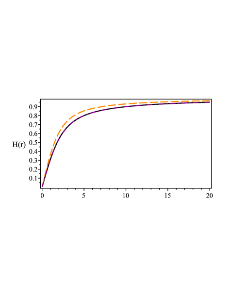
Figure 1: The Higgs profile. Top: the solution given by (45) (dashed orange line). Bottom: the solutions given by (35) (dotted purple line) and (39) (long-dashed red line for $n=2$, and space-dashed blue line for $n=3$). In both pictures, the usual profile Eq. (27) is also shown (solid black line), for comparison.

Now, following our prescription, we choose the deformation function as

$$f\left(\mathcal{H}\right)=\frac{\sin\left(\mathcal{H}\left(r\right)\right)}{\sin\left(1\right)}\text{.}$$ (48)

Then, by combining eqs. (45) and (48), we get that the deformed solution for $\mathcal{H}\left(r\right)$ reads as

$$\mathcal{H}\left(r\right)=H_{{}_{tHP}}\left(r\right)\text{,}$$ (49)

i.e., it is the usual ’t Hooft-Polyakov solution, whereas the corresponding deformed solution for $\mathcal{W}\left(r\right)$ is

$$\mathcal{W}\left(r\right)=\frac{r}{\sqrt{3w_{0}\sinh^{2}\left(r\right)-\left(3w_{0}-1\right)r^{2}}}\text{,}$$ (50)

exactly the solution previously studied in Eq. (31). Hence, the auxiliary functions $\mathcal{P}\left(r\right)$ and $\mathcal{N}\left(r\right)$ are given by eqs. (32) and (33), respectively.

The overall conclusion is that, by choosing suitable deformation functions, both completely and partially analytical monopole configurations can be deformed into a new analytical one.

In the sequel, we depict all the solutions we have found and compare them with the usual ’t Hooft-Polyakov one, commenting on the main features of the new profiles. The solutions for the Higgs field are shown in Fig. 1, which reveals that all the profiles exhibit the same general behavior, reaching their boundary values monotonically, whilst spreading over different distances.

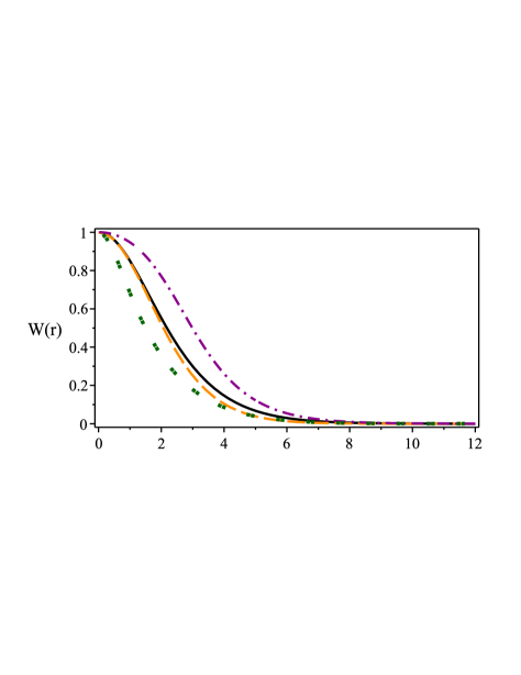
Figure 2: The gauge profile. Top: the solutions given by Eq. (31) for $w_{0}=1/10$ (dot-dashed dark-purple line), and $w_{0}=1$ (double-dotted green line). The numerical profile related to the Eq. (45) is also shown (dashed orange line for $w_{0}=1/3$). Bottom: the profiles given by (36) and (42). Here, the conventions are the same as in Fig. 1, with $C_{1}=1$.

In Fig. 2, we depict the solutions for the gauge field. Here, by plotting Eq. (31), we identify the way the integration constant coming from (24) controls the characteristic length of the deformed solutions: the profiles for $w_{0}>1/3$ spread over smaller distances, while exhibiting greater cores for $0<w_{0}<1/3$.

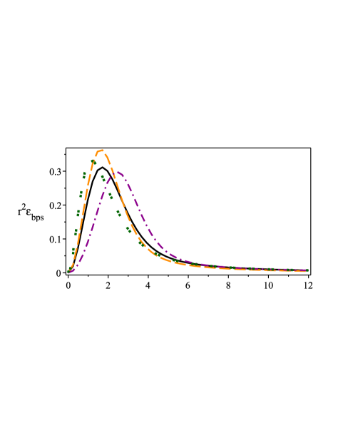
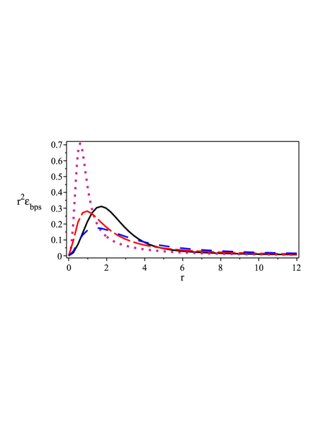
Figure 3: The product $r^{2}$ times the BPS energy density. Conventions as in Fig. 2.

Fig. 3 displays the results for the product $r^{2}$ times the BPS energy densities. These profiles are important, since the enclosed area gives (within a constant factor of $4\pi$) the energy of the BPS monopoles. In general, the solutions we have found are rings, i.e., they reach the corresponding amplitudes at some finite distance $R$ from the origin.

Finally, we point out that the new solutions we have found, despite well-behaved, are of the type $H\left(r\right)$ or $H\left(r\right).$ To obtain the inverse function, $r(H)$ or $r(H),$ provides fairly complicated relations. This way, we have preferred to express $M$ or $M$ as explicit functions of $r$. This fact does not prevent the existence of simpler configurations for $r(H)$, which were still not found out, however.

V Ending comments

In this work, we have established a deformation prescription consistent with the generalized self-dual Yang-Mills-Higgs scenario presented by some of us in a recent paper pau . Here, starting from well-known BPS field profiles, the deformation procedure allows to obtain new self-dual solutions standing for the magnetic monopoles arising within a non-Abelian-Higgs model endowed by a particular positive function $M$. It is worthwhile to point out that the initial configuration can be completely or partially analytical, the final scenario possessing exact solutions for both gauge and scalar fields.

We have checked our algorithm by studying some illustrative examples. The first two cases we have considered were entirely analytical, one based on the usual ’t Hooft-Polyakov solution, the other based on the nontrivial solution introduced in PLB . In the sequel, we have extended our work for a partially analytical configuration. It is important to point out that we have implemented a deformation prescription which gives legitimate new self-dual solutions of a different model with similar BPS equations. Such deformed solutions can not be attained by a trivial redefinition of the standard fields.

The results we have found are depicted in figs. 1, 2, and 3, the overall conclusion being that the deformed profiles behave in the same general way their standard counterpart do. In figs. 2 and 3, we have also identified the way the constant of integration $w_{0}$ affects the resulting profiles.

We are now investigating the possibility to develop a deformation procedure applicable to the study of self-dual Maxwell-Higgs, Chern-Simons-Higgs and Maxwell-Chern-Simons-Higgs vortices. We hope to report on this in the near future.

The authors thank CAPES, CNPq and FAPEMA (Brazilian agencies) for partial financial support.

References

- (1) N. Manton and P. Sutcliffe, Topological Solitons (Cambridge University Press, Cambridge, England, 2004).
- (2) E. Bogomol’nyi, Sov. J. Nucl. Phys. 24 (1976) 449. M. Prasad and C. Sommerfield, Phys. Rev. Lett. 35 (1975) 760.
- (3) D. Finkelstein, J. Math. Phys. 7 (1966) 1218.
- (4) H. B. Nielsen and P. Olesen, Nucl. Phys. B 61 (1973) 45.
- (5) G. ’t Hooft, Nucl. Phys. B 79 (1974) 276. A. M. Polyakov, JETP Lett. 20 (1974) 194.
- (6) C. Armendariz-Picon, T. Damour and V. Mukhanov, Phys. Lett. B 458 (1999) 209.
- (7) V. Mukhanov and A. Vikman, J. Cosmol. Astropart. Phys. 02 (2005) 004.
- (8) A. Sen, J. High Energy Phys. 07 (2002) 065.
- (9) C. Armendariz-Picon and E. A. Lim, J. Cosmol. Astropart. Phys. 08 (2005) 007.
- (10) J. Garriga and V. Mukhanov, Phys. Lett. B 458 (1999) 219. R. J. Scherrer, Phys. Rev. Lett. 93 (2004) 011301. A. D. Rendall, Classical Quantum Gravity 23 (2006) 1557.
- (11) D. Bazeia, E. da Hora, C. dos Santos and R. Menezes, Phys. Rev. D 81 (2010) 125014. D. Bazeia, E. da Hora, R. Menezes, H. P. de Oliveira and C. dos Santos, Phys. Rev. D 81 (2010) 125016. C. dos Santos and E. da Hora, Eur. Phys. J. C 70 (2010) 1145; Eur. Phys. J. C 71 (2011) 1519. C. dos Santos, Phys. Rev. D 82 (2010) 125009. D. Bazeia, E. da Hora and D. Rubiera-Garcia, Phys. Rev. D 84 (2011) 125005. D. Bazeia, E. da Hora, C. dos Santos and R. Menezes, Eur. Phys. J. C 71 (2011) 1833. C. dos Santos and D. Rubiera-Garcia, J. Phys. A 44 (2011) 425402. D. Bazeia, R. Casana, E. da Hora and R. Menezes, Phys. Rev. D 85 (2012) 125028. C. Adam, L. A. Ferreira, E. da Hora, A. Wereszczynski and W. J. Zakrzewski, JHEP 1308 (2013) 062.
- (12) E. Babichev, Phys. Rev. D 74 (2006) 085004; Phys. Rev. D 77 (2008) 065021. C. Adam, N. Grandi, J. Sanchez-Guillen and A. Wereszczynski, J. Phys. A 41 (2008) 212004. C. Adam, J. Sanchez-Guillen and A. Wereszczynski, J. Phys. A 40 (2007) 13625; Phys. Rev. D 82 (2010) 085015. C. Adam, N. Grandi, P. Klimas, J. Sanchez-Guillen and A. Wereszczynski, J. Phys. A 41 (2008) 375401. C. Adam, P. Klimas, J. Sanchez-Guillen and A. Wereszczynski, J. Phys. A 42 (2009) 135401. C. Adam, J. M. Queiruga, J. Sanchez-Guillen and A. Wereszczynski, Phys. Rev. D 84 (2011) 025008; Phys. Rev. D 84 (2011) 065032. P. P. Avelino, D. Bazeia, R. Menezes and J.G.G.S. Ramos, Eur. Phys. J. C 71 (2011) 1683. C. Adam and J. M. Queiruga, Phys. Rev. D 84 (2011) 105028; Phys. Rev. D 85 (2012) 025019. C. Adam, C. Naya, J. Sanchez-Guillen and A. Wereszczynski, Phys. Rev. D 86 (2012) 085001; Phys. Rev. D 86 (2012) 045015.
- (13) M. Andrews, M. Lewandowski, M. Trodden and D. Wesley, Phys. Rev. D 82 (2010) 105006. D. Bazeia, J. D. Dantas, A. R. Gomes, L. Losano and R. Menezes, Phys. Rev. D 84 (2011) 045010. D. Bazeia and R. Menezes, Phys. Rev. D 84 (2011) 105018. D. Bazeia, E. da Hora and R. Menezes, Phys. Rev. D 85 (2012) 045005. D. Bazeia, A. S. Lobão Jr. and R. Menezes, Phys. Rev. D 86 (2012) 125021.
- (14) D. Bazeia, L. Losano and J. M. C. Malbouisson, Phys. Rev. D 66 (2002) 101701(R). C. A. Almeida, D. Bazeia, L. Losano and J. M. C. Malbouisson, Phys. Rev. D 69 (2004) 067702. D. Bazeia and L. Losano, Phys. Rev. D 73 (2006) 025016.
- (15) D. Bazeia, M. A. Gonzalez Leon, L. Losano and J. Mateos Guilarte, Phys. Rev. D 73 (2006) 105008.
- (16) D. Bazeia, L. Losano, J. M. C. Malbouisson and R. Menezes, Physica D 237 (2008) 937. D. Bazeia, L. Losano, R. Menezes and M. A. M. Souza, EPL 87 (2009) 21001. D. Bazeia, L. Losano, J. M. C. Malbouisson and J. R. L. Santos, Eur. Phys. J. C 71 (2011) 176.
- (17) V. I. Afonso, D. Bazeia, M. A. Gonzalez Leon, L. Losano and J. Mateos Guilarte, Phys. Rev. D 76 (2007) 025010.
- (18) L. Losano, J. M. C. Malbouisson, D. Rubiera-Garcia and C. dos Santos, EPL 101 (2013) 31001.
- (19) R. Casana, M. M. Ferreira Jr. and E. da Hora, Phys. Rev. D 86 (2012) 085034.
- (20) J. Bagger and E. Witten, Nucl. Phys. B 222 (1983) 1; C. M. Hull, A. Karlhede, U. Lindstrom, and M. Rocek, Nucl. Phys. B 266 (1986) 1.
- (21) R. Casana, M. M. Ferreira Jr., E. da Hora and C. dos Santos, Phys. Lett. B 722 (2013) 193.