Charge transfer satellites in x-ray spectra of transition metal oxides

Abstract

Strongly correlated materials such as transition metal oxides (TMOs) often exhibit large satellites in their x-ray photoemission (XPS) and x-ray absorption spectra (XAS). These satellites arise from localized charge-transfer (CT) excitations that accompany the sudden creation of a core hole. Here we use a two-step approach to treat such excitations in a localized system embedded in a condensed system and coupled to a photoelectron. The total XAS is then given by a convolution of a spectral function representing the localized excitations and the XAS of the extended system. The local system is modeled roughly in terms of a simple three-level model, leading to a double-pole approximation for the spectral function that represents dynamically weighted contributions from the dominant neutral and charge-transfer excitations. This method is implemented using a resolvent approach, with potentials, radial wave-functions and matrix elements from the real-space Green’s function code feff, and parameters fitted to XPS experiments. Representative calculations for several TMOs are found to be in reasonable agreement with experiment.

I Introduction

Shake-up excitations in x-ray absorption (XAS) and x-ray photoemission spectra (XPS) have long been of interest.(Åberg, 1967; de Groot et al., 1990; van Veenendaal and Sawatzky, 1993) These excitations are generated by the intrinsic response of a system to a suddenly created core hole, and are reflected in satellite peaks in the spectra. Examples in XAS range from edge-singularities in metals,(Nozières and De Dominicis, 1969) to many-body amplitude factors in x-ray absorption fine structure.(Rehr and Albers, 2000) Recently such satellites have also been found to explain the extrinsic and intrinsic losses and interference effects in XPS experiments.(Guzzo et al., 2011; Söderström et al., 2012) However, these effects are relatively small in weakly-correlated materials, where the dominant excitations are plasmons. In those cases the satellite amplitudes are of order 10% of the main peak and become negligible near absorption thresholds in the adiabatic limit.(Rehr et al., 2007) Consequently, broadened single-particle theories with a core hole can be good approximations.(Rehr et al., 2009; Gunnarsson and Lundqvist, 1976; Jones and Gunnarsson, 1989; Hermann et al., 2013) In contrast, dramatic satellites comparable in strength to the main peak are typically observed in the spectra of correlated materials such as TMOs and high-temperature superconductors. These satellites are often attributed to localized charge-transfer (CT) excitations.(de Groot and Kotani, 2008) In such cases the one-particle approximation fails dramatically in the near-edge region. Several approaches with various degrees of sophistication have been introduced to address this behavior. For example, the “charge-transfer multiplet approach” treats strong correlations locally, with solid-state effects modeled by crystal-field parameters.(de Groot, 2005) Configuration interaction techniques have also been applied to small clusters,(Ikeno et al., 2009) but these methods are computationally intensive.

Our goal in this work is to develop a simple yet practical, semi-quantitative approach to model both local correlations and solid-state effects to explain these excitations. Our approach is based on a simplified two-step model with a localized system embedded in a solid, and coupled to a photoelectron. The approach incorporates both localized charge-transfer excitations and long-ranged plasmon excitations. In particular, our method combines the model of localized excitations introduced by Lee, Gunnarsson and Hedin (LGH),(Lee et al., 1999) with the treatment of solid-state effects and other inelastic losses as in the real-space Green’s function approach used in the feff9 XAS code.(Rehr et al., 2009) As a justification for this separation we note that the localized and extended excitations are spatially and energetically decoupled. Our main result is an expression for the XAS of charge-transfer systems as a convolution of an effective spectral function $A_{L}(\omega,\omega^{\prime})$ that contains the localized CT excitations, and an approximation for the XAS of extended systems $\tilde{\mu}(\omega)$ that builds in long-range, extrinsic inelastic losses

$$\mu(\omega)=\int d\omega^{\prime}\,A_{L}(\omega,\omega^{\prime})\,\tilde{\mu}(\omega-\omega^{\prime})\equiv A_{L}*\tilde{\mu}.$$ (1)

As discussed by Kas et al.,(Kas et al., 2007) $\tilde{\mu}(\omega)$ is related to the quasi-particle XAS by an analogous convolution $\tilde{\mu}=A_{Q}*\mu$. At low energies compared to the plasma frequency, plasmon satellites become negligible and $\tilde{\mu}(\omega)\approx\mu(\omega)$, i.e. the spectra calculated in the presence of a core hole. Within the simplest three-level model for the localized system, the CT spectral function $A_{L}$ has two energy-dependent peaks separated by a characteristic charge-transfer energy splitting $\delta E$ which is typically a few eV. Our result in Eq. (1) is similar to the formulation of Calandra et al.,(Calandra et al., 2012) where the spectral function is taken to be the XPS spectra $A_{L}(\omega,\omega^{\prime})=\sigma(\omega-\omega^{\prime})$. In contrast the present approach makes use of an explicit model for the localized system and also approximates dynamic effects, such as the crossover from the adiabatic to the sudden limit. We have applied this method systematically to a number of 3d TMOs, and obtain results in reasonable agreement with experiment and other calculations.(Calandra et al., 2012; Wu et al., 2004)

II Theory

II.1 LOCAL MODEL

Our model for the localized system is adapted from the three-level tight-binding model of Lee, Gunnarsson and Hedin (referred to here as LGH), Lee et al. (1999) which is only briefly summarized here. For clarity we adopt similar notation and some key formulae are reproduced in the Appendix; we refer to original paper (Lee et al., 1999) for additional details. The LGH model can be extended to a more realistic description, for example, using the Haydock recursion scheme(Haydock and Kelly, 1973) applied to a tight-binding Hamiltonian, and keeping only the leading iterations. Nevertheless, the simplified LGH model captures the essential physics of the charge-transfer process. As illustrated in Fig. 1, the levels include a strongly localized $d$ level, a less localized ligand level $L$, and a deep core level $c$. Physically, this local model represents a system in which upon photoecxitation, a localized level $d$ is pulled below the ligand level $L$ due to the Coulomb interaction with the core hole. As a result, there is a finite probability that the electron originally in the $L$ state is transferred to the $d$ state. This process corresponds to the lowest energy main peak (“shake-down”) in the photoemission process and strongly screens the core hole. There is also a finite probability that the electron will remain in level $L$, corresponding to the satellite peak and a less screened core hole. The effective spectral function is determined from the relative probabilities of these two processes.

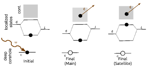
Figure 1: Schematic representation of the three-level model (core state and two localized states): the labels are d - transition metal 3d level; L - ligand valence state, cont - continuum states; $\varepsilon$ - photoelectron kinetic energy.

The Hamiltonian of the full system is separated as

$$\mathcal{H}=\mathcal{H}_{0}+T+V+\Delta,$$ (2)

where ${\cal H}_{0}$ is the Hamiltonian of the local system, $T$ is the kinetic energy of the photoelectron, $V$ is the Coulomb interaction between the photoelectron and the local system, and $\Delta$ is the coupling to the x-ray field. In detail

$${\cal H}_{0} = \sum_{i}\varepsilon_{i}n_{i}+\sum_{l}U_{l}n_{c}n_{l}+t(c^{\dagger}_{d}c_{L}+hc),$$

$$V = \sum_{{\bf kk}^{\prime}}\left[\sum_{i}n_{i}V^{i}_{{\bf kk}^{\prime}}-V^{c}_{{\bf kk}^{\prime}}\right]c_{\bf k}^{\dagger}c_{\bf k^{\prime}},$$

$$\Delta = \sum_{\bf k}M_{c{\bf k}}\,[c_{\bf k}^{\dagger}c_{c}+hc\,].$$ (3)

Here $i=(c,d,L)$, $l=(d,L)$, $\varepsilon_{d},\,\varepsilon_{L}$, and $\varepsilon_{c}$ are, respectively, the bare energies of the $d$, $L$ and $c$ levels, $U_{d}$ and $U_{L}$ represent, respectively, the Coulomb interaction between the core hole and the $d$ and $L$ levels, and $t$ is a hopping matrix element, which we approximate by just one value, $k$ and $k^{{}^{\prime}}$ are wave vectors of continuum states. Implicit in this model is the constraint $n_{d}+n_{L}=1$, so that ${\cal H}_{0}$ can be simplified in terms of a single Hubbard-like parameter $U=U_{d}-U_{L}$. Similarly, $n_{c}=0$ when the core hole is present and only the difference in the potentials $V_{sc}({\bf r})=V_{L}({\bf r})-V_{d}({\bf r})$ is needed in Eq. (5) to represent the change in potential when the electron hops from the ligand level $L$ to the localized $d$ level. The scattering matrix elements $V_{kk^{{}^{\prime}}}$ are given by $\langle\vec{k}|V_{sc}({\bf r})|\vec{k}^{\prime}\rangle$, and $U=\int d^{3}r\,\rho_{c}({\bf r})V({\bf r})\approx V(0)$, since the core charge $\rho_{c}$ is highly localized. Throughout this paper we will use Hartree atomic units $e=\hbar=m=1$ unless otherwise specified.

The excited states of this local model $|\Psi_{sk}^{f}\rangle$, with $s=1$ and 2, can be calculated exactly within a two-particle basis $|\psi_{s}\rangle|\psi_{k}\rangle$, using the resolvent approach of LGH

$$|\Psi_{sk}^{f}\rangle=\left[1+\frac{1}{E-\mathcal{H}_{0}-T-V-i\eta}V\right]|\psi_{s}\rangle|\psi_{k}\rangle,$$ (4)

where $|\psi_{s}\rangle$ correspond to the eigenstates of $\mathcal{H}_{0}$ [see Eq. (14)] with a full core-hole $n_{c}=0$. Following LGH we also represent the local potential by

$$V_{sc}({\bf r})=\begin{cases}[-V_{3d}(r)+\frac{1}{R_{0}}]/\varepsilon_{0}&r<R_{0}\\ 0&r>R_{0}.\end{cases}$$ (5)

Here $V_{3d}(r)$ is the potential of the $d$ level calculated using 3d wave functions from feff9,(Rehr et al., 2009) and the $1/R_{0}$ term crudely represents the potential of the ligand charge shell. The constant $\varepsilon_{0}$ is chosen so that $U=-V_{sc}(0)$. Since $V_{3d}(0)\gg 1/R_{0}$, $\varepsilon_{0}\approx V_{3d}(0)/U$. The parameters used in our sample calculations are given in Table 1, with details on how they are obtained given in Sec.  II.2. The scattering potentials $V_{sc}(r)$ are shown in Fig. 2. These parameters are calculated using feff wave functions and values of $R_{0}$ from Table 1 which represent distances between absorber and ligand atoms. The scattering potential is set to zero beyond $R_{0}$.

Table 1: Parameters used in the local model: $U,t$ and $\delta E$ for MnO, FeO, CoO, NiO and CuO are fit to XAS experiments (Ref. Calandra et al., 2012; Wu et al., 2004, see Sec. II.2), $R_{0}$ is obtained by averaging the distance between absorber and ligand atoms, $\varepsilon_{0},\delta E,\phi$ and $r_{00}$ were calculated using Eq. (17), (A) and (19).

	$U$(eV)	$t$(eV)	$R_{0}$(a.u.)		$\varepsilon_{0}$	$\delta E$(eV)	$\phi=\theta$	$r_{00}$
MnO	11.0	1.6	2.23		3.16	6.3	0.26	3.0
FeO	9.7	1.9	2.14		3.83	6.1	0.33	1.7
CoO	8.9	1.5	2.13		4.38	5.3	0.29	2.3
NiO	10.6	2.1	2.08		3.65	6.8	0.34	1.5
CuO	13.0	1.5	2.23		3.03	7.2	0.21	5.4

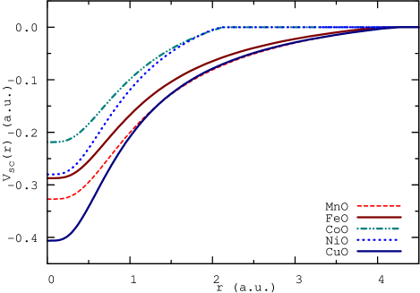
Figure 2: Photoelectron scattering potentials $V_{sc}(r)$ see Eq. 5 for MnO, FeO, CoO, NiO and CuO

The matrix elements $V_{kk^{\prime}}$ of the scattering potential are presented in Fig. 4 and compared with the analytic form discussed in LGH. Note that the numerical calculations are in good agreement with the analytical form except at low energies. The matrix elements $V_{kk^{\prime}}$ for NiO and CoO are similar, due to the similarity of their scattering potentials $V_{sc}(r)$ (see Fig. 2). The radial transition matrix elements (see Fig. 3) are given by

$$M_{ck}\propto\sqrt{(\varepsilon_{k}-\varepsilon_{c})}\int\mathrm{d}{r}\,r^{2}\,\psi_{c}(r)\,r\,u_{lk}(r),$$ (6)

where the radial wave functions $u_{lk}(r)$ are

$$u_{lk}(r)=\begin{cases}\tilde{u}_{lk}(r)&r<r_{mt}\\ \sqrt{2/L}\,[h_{l}(kr)e^{i\delta_{lk}}+c.c.]&r>r_{mt},\end{cases}$$ (7)

and are calculated from subroutines in feff9(Rehr et al., 2009). Here, $\tilde{u}_{lk}(r)$ corresponds to the regular solution for angular momentum $l$ at the origin, matched to solutions beyond $r_{mt}$ in terms of spherical Hankel functions $h_{l}(kr)$, and $\delta_{lk}$ is the partial wave phase shift. Boundary conditions within a sphere of large radius $L=40$ a.u. and an exponential grid with $0.01$ a.u. step are used to obtain smooth results for the matrix elements.

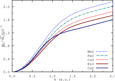
Figure 3: Dipole matrix elements $M_{ck}$ in Eq.  (6) for MnO, FeO, CoO, NiO and CuO, calculated from feff.

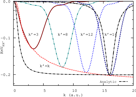
Figure 4: Matrix elements $V_{kk^{{}^{\prime}}}$ for CoO. For comparison, the LGH analytical form [Ref. Lee et al., 1999] of $V_{kk^{\prime}}$ for $k=k^{{}^{\prime}}$ and $k^{{}^{\prime}}=16$ au is also shown, calculated with parameters: $\tilde{V}=-0.79$ a.u., $R_{sd}=1.01$ au and $R_{s}=3.97$ au.

Figure 5: Ratios between full photocurrent Eq. (16) and photocurrent in the sudden limit Eq. (10) for the main $R_{1}(\omega)$ (top) and satellite $R_{2}(\omega)$ (bottom) peaks Eq. (9) for MnO, FeO, CoO, NiO and CuO. Note the significant dynamic variation at low energies while the adiabatic limit is reached around $30$ eV.

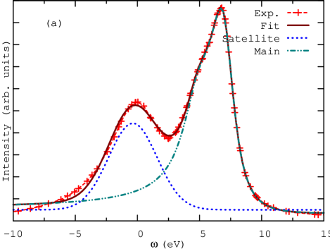
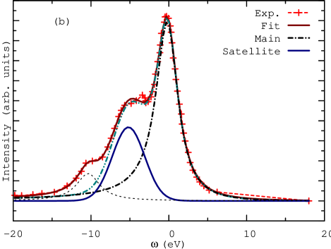
Figure 6: (a) Recent XPS experiment [Ref. Calandra et al., 2012] of NiO 1s edge, with subtracted plasmon background. (b) XPS spectra [Ref. Parmigiani and Sangaletti, 1999] for CoO.

II.2 CT PARAMETERS

Due to the simplicity of our model, there is no simple correspondence to the tight-binding parameters of a more realistic system. Nevertheless, the charge-transfer parameters of the three level system can be chosen to fit the main ($s=1$) and satellite ($s=2$) peaks in XPS experiments. The energy difference between these two peaks is defined as $\delta E$, while $w_{1}/w_{2}$ refers to the ratio of intensity of the main to the satellite peak and is given by Eq. (17) and (18). For NiO we fit these quantities to the 1s XPS edge data (Fig. 6 a) of Calandra et al.(Calandra et al., 2012) Due to band splitting, the main peak is bimodal and asymmetric. Thus we simply fit its strength to two complex Lorentzians, while the satellite peak was fit with a single Gaussian. The plasmon peaks at about $-25$ eV are ignored, since they are implicitly included in $\tilde{\mu}$ and are only important at high energies. Solving Eq. (17) and (18) yields estimates for $U$ and $t$. For CoO we used 3s XPS edge data,(Parmigiani and Sangaletti, 1999) since 1s results are not available. As in the case of NiO, we also subtracted the peak near $-12$ eV. We fit the main peak with a single complex Lorentzian while the satellite was fit with a single Gaussian. In the case of MnO, FeO and CuO we used 3s XPS experimental data (Galakhov et al., 1999) as 1s are not available. For MnO and FeO we fit the main and satellite peaks with complex Lorentzians, following the same procedure for estimating parameters for the LGH model described above. We also tried to estimate the hopping parameter $t$ from the width of the projected $d$-density of states of the absorber as obtained from the ldos module in feff, but these results only agree qualitatively with the fits given in Table 1.

III Results

Assuming isotropic XPS and summing over all directions, the XAS is simply related to the XPS photocurrent

$$\mu(\omega)=\sum_{sk}J_{k}^{s}(\omega)\propto\sum_{s}\frac{1}{k_{s}}|M(s,k_{s})|^{2},$$ (8)

where $M(s,k)\equiv\langle\Psi_{sk}^{f}|\Delta|\Psi_{0}\rangle$ is obtained from the resolvent formula in Eq. (4)), where $k_{s}=\sqrt{2(\omega+E_{0}-E_{s})}$, and $E_{s}$ are obtained from eigenvalues of the model Hamiltonian from Eq. (17). To simplify the discussion of the dynamical effects, we introduce the ratio $R_{s}(\omega)$ between the calculated photocurrents at a given photon energy, and the photocurrent $J^{0}_{i}(\omega)$ in the sudden approximation,

$$R_{s}(\omega)=\sum_{k}J^{s}_{k}(\omega)/J^{0}_{s}(\omega).$$ (9)

where the sudden-limit is

$$\begin{split}J^{0}_{s}(\omega)&=\frac{1}{k_{s}}\sum_{k}|M_{ck}w_{s}|^{2}\delta(\omega-\epsilon_{k}+E_{0}-E_{s})\\ &=w_{s}^{2}\,\tilde{\mu}(\omega-E_{s}),\end{split}$$ (10)

and $J^{s}_{k}(\omega)$ is given my Eq. (16). Here $\tilde{\mu}$ implicitly includes the effects of long-range inelastic losses in the XAS, $M_{ck}$ is given by Eq. (6), and the weights $w_{s}$ are given by Eq. (18). Thus the total XAS can be written as

$$\begin{split}\mu(\omega)&=\sum_{sk}{|M(s,k)|^{2}}\delta(\omega-\epsilon_{k}+E_{0}-E_{s})\\ &=\sum_{s}J_{s}^{0}(\omega)R_{s}(\omega).\end{split}$$ (11)

Fig. 5 shows $R_{s}(\omega)$ for a number of TMOs. Note that there is a significant “overshoot” at low energies, while above about 30 eV, $R_{s}(\omega)$ tends to the sudden limit. This behavior arises from the interplay between intrinsic and extrinsic effects represented by the first and second terms in Eq. (4). The overshoot is a fairly small correction to the adiabatic limit, since the interaction between the scattered electron and the core hole is relatively small as a result of screening of the core hole by the charge transfer process.

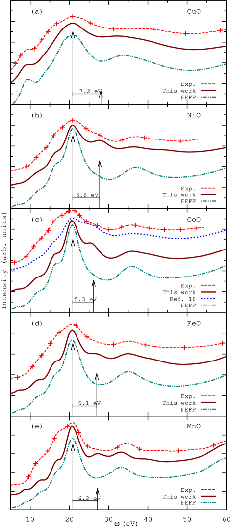
Figure 7: Comparison of the experimental XAS [Ref. Calandra et al., 2012; Wu et al., 2004], convolution using three level model (LGH), to single particle (feff) calculation for (a) MnO, (b) FeO, (c) CoO, (d) NiO and (e) CuO. And Calandra approach [Ref. Calandra et al., 2012] for CoO. Main and satellite peak position and intensities are shown with arrows. Intensity ratio is equal to $r_{00}$, see Table 1

.

In our calculations, $\tilde{\mu}(\omega-E_{s})$ is the total XAS spectrum calculated from feff9.(Rehr et al., 2009) Thus one finally obtains the convolution formula of Eq. (1) with the spectral function $A_{L}(\omega,\omega^{{}^{\prime}})$ given by

$$A_{L}(\omega,\omega^{\prime})=\frac{1}{D}\sum_{s}{w_{s}^{2}R_{s}(\omega)\delta(\omega-\omega^{\prime}-\omega_{s})},$$ (12)

where the normalization constant $D=\sum w_{s}^{2}R_{s}(\omega)$. Calculations of $R_{s}(\omega)$ were performed using the resolvent formula (see Eq. (4)) with a Hamiltonian matrix with indices $s,k$ and 80 $k$-points of dimension $160\times 160$. Calculations of the XAS for NiO were carried out using both our two step model and, for comparison, a convolution with a multiple Lorentzian fit to the XPS as in Calandra et al.(Calandra et al., 2012) Results for CoO are presented in Fig. 7 (c) and show that the two methods are numerically similar, with small differences arising from differences in broadening between two experiments. To account for differences in broadening ($\Delta\Gamma$) of the main and satellite peaks in CoO, which can be seen in XPS experimental data (see Fig. 6), broadening of the satellite peak was carried out with value $\Delta\Gamma=0.4$ eV. Results for CuO and NiO are presented in Fig. 7 (a, b) using values of $\Delta\Gamma$ $0.6$ and $1$ eV respectively. Calculations of XAS for FeO and MnO are presented in Fig. 7 (d, e), values of $\Delta\Gamma$ are $1.46$ and $1.1$ eV respectively. The effect of CT satellites are clearly seen in the Fig. 7. In particular the satellite peak transfers oscillator strength from the main peak and fills in missing spectral weight in one particle calculations above the main peak. On the other hand, the treatment here is only semi-quantitative as the satellite peaks seen in the experimental XAS are more broadened than can be represented by a two-peaked spectral function. For MnO, the parameters for the LGH model were fit to the XPS experiments shown in Fig. 6, and are given in Table 1.

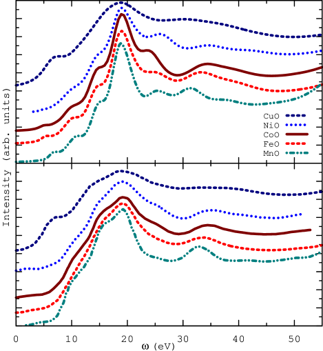
Figure 8: Comparison of spectra calculated using three level system (LGH) (top) and experimental [Ref. Wu et al., 2004; Calandra et al., 2012] XAS data (bottom) for a number of TMOs.

IV Conclusions

We have developed a simplified, semi-empirical model of the effects of charge-transfer excitations in XAS, thus extending the formulation of Lee, Gunnarsson, and Hedin.(Lee et al., 1999) The spectra are modeled by a localized three-state system coupled to a photoelectron, and implemented using the feff9 real-space Green’s function code to include solid state and extrinsic losses. The final spectrum is a convolution of a single-particle XAS calculated using feff, with a frequency-dependent spectral function consisting of two delta functions that represents the localized charge-transfer excitations. We find fairly good agreement between our results and the XAS at the metal K edges for number of TMOs (see Fig. (8)). In these spectra, the presence of charge transfer satellites are clearly seen by comparing the total and single-particle XAS, where such peaks are missing in the latter. The convolution of the single-particle spectra from feff with the CT spectral function $A_{L}(\omega)$ reproduces fairly well the peaks at higher energies with an energy splitting $\delta E$. However, the CT satellite peaks in the model spectra are sharper, which is likely an artifact of the two-delta function model for the spectral function. From Fig. (8) one can see that there is a noticeable discrepancy between experimental and calculated spectra in the pre-edge region: in some cases there are missing peaks, while in others the intensities are smaller. These differences might be due to the spherical muffin-tin(Slater, 1937) approximation of the scattering potential, as full potential single particle calculations(Calandra et al., 2012) for CoO and NiO have greater intensities in the pre-edge region. However the main goal of this paper was to approximate the CT satellite peaks. Further work is needed to obtain ab initio values of the parameters used in the model. In principle these could be found using constrained DFT or constrained RPA methods.

Appendix A LOCAL MODEL

Here we briefly summarize the details of the sudden approximation for the local model, closely following the methodology and notation of LGH.(Lee et al., 1999) The initial state $|\Psi_{0}\rangle$ is the ground state of $\mathcal{H}_{0}$ with $n_{c}=1$

$$|\Psi^{0}\rangle=-\sin(\theta)|\psi_{c}\rangle|\psi_{a}\rangle+\cos(\theta)|\psi_{c}\rangle|\psi_{b}\rangle.$$ (13)

The final states $|\Psi_{sk}^{f}\rangle$ are given by Eq. (4), where $|\psi_{1}\rangle$ and $|\psi_{2}\rangle$ are the eigenstates of $\mathcal{H}_{0}$ with $n_{c}=0$, and can be parameterized conveniently in terms of mixing angles $\theta$ and $\phi$

$$|\psi_{s}\rangle = \begin{cases}\cos(\phi)|\psi_{a}\rangle-\sin(\phi)|\psi_{b}\rangle,\mbox{ }s=1,\\ \sin(\phi)|\psi_{a}\rangle+\cos(\phi)|\psi_{b}\rangle,\mbox{ }s=2,\\ \end{cases}$$ (14)

where

$$\tan(2\theta) = 2t/(\varepsilon_{a}-\varepsilon_{b}+U),$$

$$\tan(2\phi) = 2t/(\varepsilon_{b}-\varepsilon_{a}),$$ (15)

and $a$ and $b$ correspond to the metal d- and oxygen p-levels. The photocurrent is then calculated using(Almbladh and Hedin, 1983)

$$J^{s}_{k}(\omega)=|\langle\Psi_{sk}^{f}|\Delta|\Psi^{0}\rangle|^{2}\delta(\omega-\varepsilon_{k}+E_{0}-E_{s}).$$ (16)

The spectrum of the model Hamiltonian is characterized by the parameters

$$\begin{split}&E_{s}=\frac{1}{2}(\varepsilon_{a}+\varepsilon_{b})\mp\delta E/2,\\ &\delta E=\sqrt{(\varepsilon_{a}-\varepsilon_{b})^{2}+4t^{2}}.\end{split}$$ (17)

We consider only the symmetric case with $\varepsilon_{a}=\varepsilon-U/2$ and $\varepsilon_{b}=\varepsilon$. The weights of main and satellite levels are then

$$w_{s}=\begin{cases}-\sin(\phi+\theta),\mbox{ }s=1\\ \mbox{ }\mbox{ }\cos(\phi+\theta),\mbox{ }s=2.\end{cases}$$ (18)

In the sudden(Lee et al., 1999) limit there is no interaction between the photoelectron and the electron on the outer level, so that the ratio of the main to the satellite peak intensities is

$$r_{00}=\lim_{\omega\to\infty}\frac{\sum_{k}J^{2}_{k}(\omega)}{\sum_{k}J^{1}_{k}(\omega)}=\cot^{2}(\phi+\theta).$$ (19)

References

- Åberg (1967) T. Åberg, Phys. Rev. 156, 35 (1967).
- de Groot et al. (1990) F. M. F. de Groot, J. C. Fuggle, B. T. Thole, and G. A. Sawatzky, Phys. Rev. B 42, 5459 (1990).
- van Veenendaal and Sawatzky (1993) M. A. van Veenendaal and G. A. Sawatzky, Phys. Rev. Lett. 70, 2459 (1993).
- Nozières and De Dominicis (1969) P. Nozières and C. T. De Dominicis, Phys. Rev. 178, 1097 (1969).
- Rehr and Albers (2000) J. J. Rehr and R. C. Albers, Rev. Mod. Phys. 72, 621 (2000).
- Guzzo et al. (2011) M. Guzzo, G. Lani, F. Sottile, P. Romaniello, M. Gatti, J. J. Kas, J. J. Rehr, M. G. Silly, F. Sirotti, and L. Reining, Phys. Rev. Lett. 107, 166401 (2011).
- Söderström et al. (2012) J. Söderström, N. Mårtensson, O. Travnikova, M. Patanen, C. Miron, L. J. Sæthre, K. J. Børve, J. J. Rehr, J. J. Kas, F. D. Vila, et al., Phys. Rev. Lett. 108, 193005 (2012).
- Rehr et al. (2007) J. J. Rehr, J. J. Kas, M. P. Prange, A. P. Sorini, L. W. Campbell, and F. D. Vila, in AIP Conf. Proc. (2007), vol. 882, p. 85.
- Rehr et al. (2009) J. J. Rehr, J. J. Kas, M. P. Prange, A. P. Sorini, Y. Takimoto, and F. D. Vila, Comp. Ren. Phys. 10, 548 (2009).
- Gunnarsson and Lundqvist (1976) O. Gunnarsson and B. I. Lundqvist, Phys. Rev. B 13, 4274 (1976).
- Jones and Gunnarsson (1989) R. O. Jones and O. Gunnarsson, Rev. Mod. Phys. 61, 689 (1989).
- Hermann et al. (2013) K. Hermann, L. Pettersson, M. Casida, C. Daul, A. Goursot, A. Koester, E. Proynov, A. St-Amant, D. Salahub, V. Carravetta, et al., Stobe-demon version 3.2 (2013).
- de Groot and Kotani (2008) F. M. F. de Groot and A. Kotani, Core Level Spectroscopy of Solids (CRC Press, 2008).
- de Groot (2005) F. M. F. de Groot, Coor. Chem. Rev. 249, 31 (2005).
- Ikeno et al. (2009) H. Ikeno, F. M. F. de Groot, E. Stavitski, and I. Tanaka, J. Phys.: Condens. Matter 21, 104208 (2009).
- Lee et al. (1999) J. D. Lee, O. Gunnarsson, and L. Hedin, Phys. Rev. B 60, 8034 (1999).
- Kas et al. (2007) J. J. Kas, A. P. Sorini, M. P. Prange, L. W. Cambell, J. A. Soininen, and J. J. Rehr, Phys. Rev. B 76, 195116 (2007).
- Calandra et al. (2012) M. Calandra, J. P. Rueff, C. Gougoussis, D. Céolin, M. Gorgoi, S. Benedetti, P. Torelli, A. Shukla, D. Chandesris, and C. Brouder, Phys. Rev. B 86, 165102 (2012).
- Wu et al. (2004) Z. Wu, D. Xian, T. Hu, Y. Xie, Y. Tao, C. Natoli, E. Paris, and A. Marcelli, Phys. Rev. B 70 (2004).
- Haydock and Kelly (1973) R. Haydock and M. J. Kelly, Surf. Sci. 38, 139–148 (1973).
- Parmigiani and Sangaletti (1999) F. Parmigiani and L. Sangaletti, J. Electron Spectrosc. and Relat. Phenom. 98, 287 (1999).
- Galakhov et al. (1999) V. R. Galakhov, S. Uhlenbrock, S. Bartkowski, A. V. Postnikov, M. Neumann, L. D. Finkelstein, E. Z. Kurmaev, A. A. Samokhvalov, and L. I. Leonyuk, eprint arXiv:cond-mat/9903354 (1999).
- Slater (1937) J. C. Slater, Phys. Rev. 51, 846 (1937).
- Almbladh and Hedin (1983) C.-O. Almbladh and L. Hedin, Handbook on synchrotron radiation, vol. 1B (North-Holland, 1983).