Phase structure and Hosotani mechanism in QCD-like theory with compact dimensions

Abstract:

We investigated the phase diagram of $SU(3)$ gauge theory in four dimension with one compact dimension by using the perturbative one-loop effective potential. Effects of the adjoint and fundamental fermions are investigated and then the rich phase structure in the quark-mass and compact-size scale is realized. Our results are qualitatively consistent with the recent lattice calculation and clearly show that the lattice calculation can be understood from the Hosotani mechanism. Moreover, we show the result obtained by using the flavor twisted boundary condition for fundamental fermion which does not break the $Z_{3}$ symmetry, explicitly.

1 Introduction

The Higgs-like particle has been discovered recently in Large Hadron Collider (LHC) [1, 2]. The one of primary interests of particle physics is to understand the mechanism of dynamical electroweak symmetry breaking. The one of the promising mechanism to explain the Higgs particle is the Hosotani mechanism [3, 4] which leads the gauge-Higgs unification.

In the Hosotani mechanism, the Higgs particle is interpreted as the fluctuation of the extra-dimensional component of the gauge field when the adjoint fermions are introduced with a periodic boundary condition (PBC) because the non-zero vacuum expectation value (VEV) of the extra-dimensional component of gauge field is realized.

Recently, same phenomena has been observed in a different context ; for example, see Ref. [5, 6, 7]. When the adjoint fermions with PBC are introduced to Quantum Chromodynamic (QCD) at finite temperature, some exotic phases are appeared. In such exotic phase, the traced fundamental Polyakov-loop $\Phi$ can have the non-trivial value and it show the spontaneous gauge-symmetry breaking. It means the realization of the Hosotani mechanism in $R^{3}\times S^{1}$ space-time as shown later.

Furthermore, we consider the flavor twisted boundary condition (FTBC) for fundamental fermions. This FTBC is considered in Ref. [8, 9] to investigate correlations between the $Z_{3}$ and chiral symmetries breaking because the $Z_{3}$ symmetry is not explicitly broken in the case with FTBC even if we introduce the fundamental fermions. In the standard fundamental fermion can not leads the spontaneous gauge symmetry breaking, but fundamental fermions with FTBC can lead the breaking as shown later.

The purpose of this talk is to explain how to understand the recent lattice simulation from the Hosotani mechanism and possibility of the spontaneous gauge symmetry breaking by the fundamental fermions. This talk is based on papers [10, 11]

2 Formalism

In this study, we use the perturbative one-loop effective potential  [12, 13] on $R^{3}\times S^{1}$ for gauge boson and fermions and then the imaginary time direction is the compacted dimension.

Firstly, we expand the $SU(N)$ gauge boson field as

$$A_{\mu} =\langle A_{y}\rangle+\tilde{A}_{\mu},$$ (1)

where $y$ stands for a compact direction, $\langle A_{y}\rangle$ is VEV and $\tilde{A}_{\mu}$ express the fluctuation part. For latter convenience, we rewrite it as

$$\langle A_{y}\rangle =\frac{2\pi}{gL}q,$$ (2)

where $g$ is gauge coupling constant and $q$’s color structure is $\mathrm{diag}(q_{1},q_{2},...,q_{N})$ and each component should be $(q_{i})_{mod~{}1}$. We note that eigenvalues of $q_{i}$ are invariant under all gauge transformations preserving boundary conditions and thus we can easily observe spontaneous gauge symmetry breaking from values of $q_{i}$.

The gluon one-loop effective potential ${\cal V}_{g}$ can be expressed as

$${\cal V}_{g} =-\frac{2}{L^{4}\pi^{2}}\sum_{i,j=1}^{N}\sum_{n=1}^{\infty}\Bigl{(}1-\frac{1}{N}\delta_{ij}\Bigr{)}\frac{\cos(2n\pi q^{ij})}{n^{4}}$$ (3)

where $q_{ij}=(q_{i}-q_{j})_{mod~{}1}$ and $N$ means the number of color degrees of freedom. The perturbative one-loop effective potential for the massive fundamental quark is expressed by using the second kind of the modified Bessel function $K_{2}(x)$ as

$${\cal V}_{f}^{\phi}(N_{f},m_{f}) =\frac{2N_{f}m_{f}^{2}}{\pi^{2}L^{2}}\sum_{i=1}^{N}\sum_{n=1}^{\infty}\frac{K_{2}(nm_{f}L)}{n^{2}}\cos[2\pi n(q_{i}+\phi)],$$ (4)

where $N_{f}$ and $m_{f}$ are the number of flavors and the mass for fundamental fermions. The perturbative one-loop effective potential for the massive adjoint quark ${\cal V}_{a}^{\phi}$ is

$${\cal V}_{a}^{\phi}(N_{a},m_{a}) =\frac{2N_{a}m_{a}^{2}}{\pi^{2}L^{2}}\sum_{i,j=1}^{N}\sum_{n=1}^{\infty}\Bigl{(}1-\frac{1}{N}\delta_{ij}\Bigr{)}\frac{K_{2}(nm_{a}L)}{n^{2}}\cos[2\pi n(q_{ij}+\phi)],$$ (5)

where $N_{a}$ and $m_{a}$ are the number of flavors and the mass for adjoint fermions.

For the gauge theory with $N_{f}$ fundamental and $N_{a}$ adjoint fermions with arbitrary boundary conditions, the total perturbative one-loop effective potential becomes

$${\cal V}={\cal V}_{g}+{\cal V}_{f}^{\phi}(N_{f},m_{f})+{\cal V}_{a}^{\phi}(N_{a},m_{a}).$$ (6)

This total one-loop effective potential contains eight parameters including the compact scale $L$, the number of colors $N$, the fermion masses $m_{f}$, $m_{a}$, the number of flavors $N_{f}$, $N_{a}$, and the boundary conditions $\phi$ for two kinds of matter fields. In this study, we keep $N=3$ and then the phase diagram is obtained in $1/L$-$m_{a}$ space with fixed $m_{f}$, $N_{f}$, $N_{a}$ and $\phi$. The reason we change $m_{a}$ while fixing $m_{f}$ is that gauge symmetry phase diagram is more sensitive to the former than the latter.

3 $SU(3)$ gauge theory with adjoint and fundamental quarks [10]

Here, we consider the case of $(N_{f},N_{a})=(0,1)$ with PBC. We note that this case has exact $Z_{3}$ symmetry because the adjoint quark dose not break the symmetry. Figure 1 shows the effective potential $[{\cal V}_{g}+{\cal V}_{a}^{0}(N_{a},m_{a})]L^{4}$ as a function of $q_{1}$ with $q_{2}=0$ for $mL=1.2$, $1.6$, $2.0$ and $3.0$ from left to right panels ($m\equiv m_{a}$).

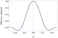
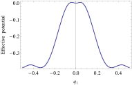
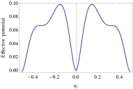
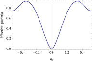
Figure 1: The one-loop effective potential of $SU(3)$ gauge theory with one flavor PBC adjoint quark as a function of $q_{1}$ with $q_{2}=0$ for $mL=1.2$ (reconfined) $1.6$ (reconfined$\leftrightarrow$split), $2.0$ (split$\leftrightarrow$deconfined) and $3.0$ (deconfined).

We can clearly see that there is the first-order phase transition in the vicinity of $mL=1.6$. This is a transition between the reconfined phase and the other gauge-broken phase, which we call the split phase.

In Fig. 2, we show the phase diagram in $L^{-1}$-$m$ plane with $(N_{f},N_{a})=(0,1)$ quark based on the perturbative one-loop effective potential.

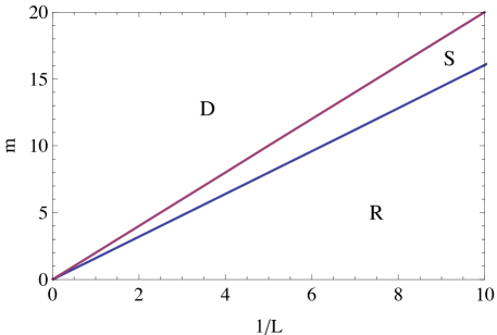
Figure 2: $L^{-1}$-$m$ phase diagram for $SU(3)$ gauge theory on $R^{3}\times S^{1}$ with one PBC adjoint quark based on one-loop effective potential. The symbol D stands for deconfined ($SU(3)$), S for split ($SU(2)\times U(1)$) and R for reconfined ($U(1)\times U(1)$) phases.

We note that, as $m$ appears as $mL$ in the potential, we have liner scaling in the phase diagram. Since we drop the non-perturbative effect in the gluon potential, we can not obtain the confined phase at small $L^{-1}$. The order of three phases in Fig. 2 (deconfined $SU(3)$ $\to$ split $SU(2)\times U(1)$ $\to$ reconfined $U(1)\times U(1)$ from small to large $L^{-1}$) is consistent with that of the lattice simulation [6, 7] except the confined phase. All the critical lines in the figure are first-order. In Fig. 3 we show a schematic distribution plot of $\Phi$ in the complex plane for each phases. In the split phase, $\Phi$ has nonzero values but in a different manner from the deconfined phase. In the reconfined phase, we have $\Phi=0$ with the vacuum which breaks the gauge symmetry.

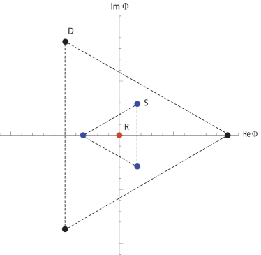
Figure 3: Schematic distribution plot of Polyakov loop $\Phi$ as a function of $\mathrm{Re}~{}\Phi$ and $\mathrm{Im}~{}\Phi$ for $SU(3)$ gauge theory with one flavor PBC adjoint quark.

From above results, we can understand the lattice results [6] from Hosotani mechanism as shown in Fig 4.

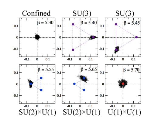
Figure 4: Comparison between distribution plot of Polyakov loop $\Phi$ on the lattice [6] and that of the one-loop effective potential for $SU(3)$ gauge theory on $R^{3}\times S^{1}$ with PBC adjoint quarks. Apart from the strong-coupling confined phase, all of the specific behavior can be interpreted as the phases we found in our analytical calculations.

The schematic figure of the fundamental quark effect to the phase diagram is shown in Fig. 5.

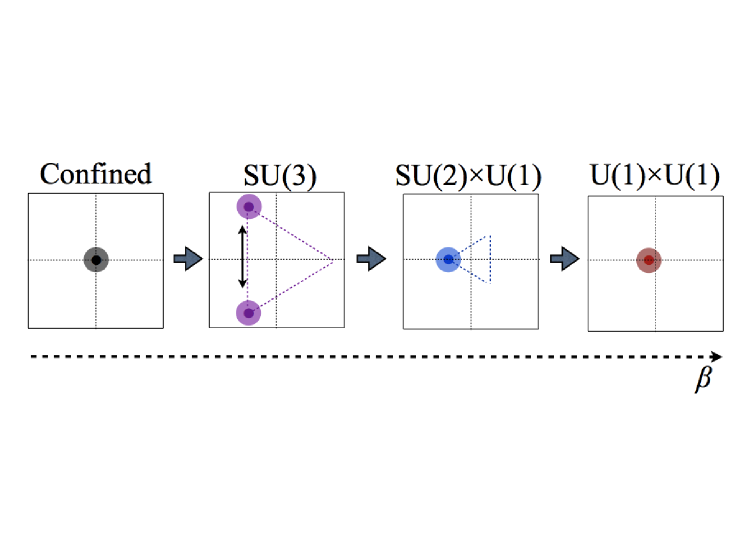
Figure 5: Prediction of distribution plot of Polyakov loop $\Phi$ based on the one-loop effective potential for $SU(3)$ gauge theory on $R^{3}\times S^{1}$ with PBC adjoint and fundamental quarks.

The reconfined phase is replaced by the pseudo-confined phase because the $Z_{3}$ symmetry is explicitly broken by the fundamental quark contributions, but the gauge symmetry breaking pattern is still same.

4 $SU(3)$ gauge theory with FTBC fundamental quarks [11]

In this section, we consider the FTBC for the fundamental fermion. Details of FTBC are shown in Ref. [8, 9].

Contour plots of the $SU(3)$ gauge theory with $N_{F,fund}=120$ FTBC fundamental quark for the gauge symmetric and broken phase are shown in Fig. 6.

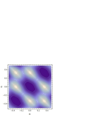
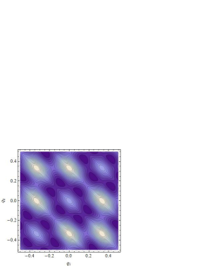
Figure 6: Contour plot of $[{\cal V}_{g}+{\cal V}_{f}]L^{4}$ in the $q_{1}$-$q_{2}$ plane for the case of $N_{F,fund}=120$ FTBC fermions. The upper panel corresponds to the $SU(3)$ deconfined phase and the lower panel does to the $SU(2)\times U(1)$ C-broken phase.

Unlike the standard fundamental quark, we can clearly see the existence of the spontaneous gauge symmetry breaking of $SU(3)\to SU(2)\times U(1)$. The distribution plot of the fundamental Polyakov-loop is shown in Fig. 7.

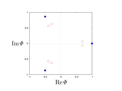
Figure 7: Distribution of the Polyakov loop in the complex plane for a $SU(3)$ gauge theory on with $N_{F,fund}=120$ FTBC fermions. Solid circles correspond to the deconfinement phase and open circles do to the gauge symmetry broken phase.

The phase diagram is shown in Fig. 8 in the $L^{-1}$-$m$ plane.

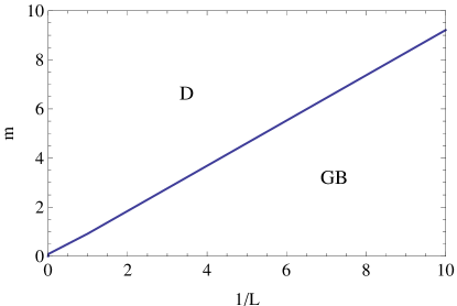
Figure 8: The phase diagram in the $L^{-1}$-$m$ plane for a $SU(3)$ gauge theory with $N_{F,fund}=120$ FTBC fermions. The symbol D stands for the deconfinement phase and GB for the $SU(2)\times U(1)$ gauge symmetry broken phase. In the gauge symmetry broken phase, charge conjugation is also spontaneously broken which can be seen from the charge-conjugation pairs.

In the case with FTBC fundamental fermions, there is no $U(1)\times U(1)$ phase, but $SU(2)\times U(1)$ phase is still exist. The $Z_{3}$ symmetry is not explicitly broken as same as the adjoint fermions and also lattice simulations are possible. Therefore, this system is very interesting to consider the gauge symmetry breaking and also the confinement-deconfinement transition.

References

- [1] G. Aad et al. [ATLAS Collaboration], Phys. Lett. B 716, 1 (2012) [arXiv:1207.7214 [hep-ex]].
- [2] S. Chatrchyan et al. [CMS Collaboration], Phys. Lett. B 716, 30 (2012) [arXiv:1207.7235 [hep-ex]].
- [3] Y. Hosotani, Phys. Lett. B 126, 309 (1983).
- [4] Y. Hosotani, Annals Phys. 190, 233 (1989).
- [5] H. Nishimura and M. C. Ogilvie, Phys. Rev. D 81, 014018 (2010) [arXiv:0911.2696 [hep-lat]].
- [6] G. Cossu and M. D’Elia, JHEP 0907, 048 (2009) [arXiv:0904.1353 [hep-lat]].
- [7] G. Cossu, H. Hatanaka, Y. Hosotani and J. -I. Noaki, arXiv:1309.4198 [hep-lat].
- [8] H. Kouno, Y. Sakai, T. Makiyama, K. Tokunaga, T. Sasaki and M. Yahiro, J. Phys. G 39 (2012) 085010.
- [9] Y. Sakai, H. Kouno, T. Sasaki and M. Yahiro, Phys. Lett. B 718, 130 (2012) [arXiv:1204.0228 [hep-ph]].
- [10] K. Kashiwa and T. Misumi, JHEP 1305, 042 (2013) [arXiv:1302.2196 [hep-ph]].
- [11] H. Kouno, T. Misumi, K. Kashiwa, T. Makiyama, T. Sasaki and M. Yahiro, Phys. Rev. D 88 (2013) 016002 [arXiv:1304.3274 [hep-ph]].
- [12] D. J. Gross, R. D. Pisarski and L. G. Yaffe, Rev. Mod. Phys. 53, 43 (1981).
- [13] N. Weiss, Phys. Rev. D 24, 475 (1981).