Sparse PCA via Covariance Thresholding

Abstract

In sparse principal component analysis we are given noisy observations of a low-rank matrix of dimension $n\times p$ and seek to reconstruct it under additional sparsity assumptions. In particular, we assume here each of the principal components ${\mathbf{v}}_{1},\dots,{\mathbf{v}}_{r}$ has at most $s_{0}$ non-zero entries. We are particularly interested in the high dimensional regime wherein $p$ is comparable to, or even much larger than $n$.

In an influential paper, [JL04] introduced a simple algorithm that estimates the support of the principal vectors ${\mathbf{v}}_{1},\dots,{\mathbf{v}}_{r}$ by the largest entries in the diagonal of the empirical covariance. This method can be shown to identify the correct support with high probability if $s_{0}\leq K_{1}\sqrt{n/\log p}$, and to fail with high probability if $s_{0}\geq K_{2}\sqrt{n/\log p}$ for two constants $0<K_{1},K_{2}<\infty$. Despite a considerable amount of work over the last ten years, no practical algorithm exists with provably better support recovery guarantees.

Here we analyze a covariance thresholding algorithm that was recently proposed by [KNV13]. On the basis of numerical simulations (for the rank-one case), these authors conjectured that covariance thresholding correctly recover the support with high probability for $s_{0}\leq K\sqrt{n}$ (assuming $n$ of the same order as $p$). We prove this conjecture, and in fact establish a more general guarantee including higher-rank as well as $n$ much smaller than $p$. Recent lower bounds [BR13, MW15a] suggest that no polynomial time algorithm can do significantly better.

The key technical component of our analysis develops new bounds on the norm of kernel random matrices, in regimes that were not considered before. Using these, we also derive sharp bounds for estimating the population covariance (in operator norm), and the principal component (in $\ell_{2}$-norm).

1 Introduction

In the spiked covariance model proposed by [JL04], we are given data ${\mathbf{x}}_{1},{\mathbf{x}}_{2},\dots,{\mathbf{x}}_{n}$ with ${\mathbf{x}}_{i}\in\mathbb{R}^{p}$ of the form:

$${\mathbf{x}}_{i} =\sum_{q=1}^{r}\sqrt{\beta_{q}}\,u_{q,i}\,{\mathbf{v}}_{q}+{\mathbf{z}}_{i}\,,$$ (1)

Here ${\mathbf{v}}_{1},\dots,{\mathbf{v}}_{r}\in\mathbb{R}^{p}$ is a set of orthonormal vectors, that we want to estimate, while $u_{q,i}\sim{\sf N}(0,1)$ and ${\mathbf{z}}_{i}\sim{\sf N}(0,{\rm I}_{p})$ are independent and identically distributed. The quantity $\beta_{q}\in\mathbb{R}_{>0}$ is a measure of signal-to-noise ratio. In the rest of this introduction, in order to simplify the exposition, we will refer to the rank one case and drop the subscript $q\in\{1,2,\dots,r\}$. Further, we will assume $n$ to be of the same order as $p$. Our results and proofs hold for a broad range of scalings of $r$, $p$, $n$, and will be stated in general form.

The standard method of principal component analysis involves computing the sample covariance matrix ${\mathbf{G}}=n^{-1}\sum_{i=1}^{n}{\mathbf{x}}_{i}{\mathbf{x}}_{i}^{{\sf T}}$ and estimates ${\mathbf{v}}={\mathbf{v}}_{1}$ by its principal eigenvector ${\mathbf{v}}_{\mbox{\tiny{\sc PC}}}({\mathbf{G}})$. It is a well-known fact that, in the high dimensional regime, this yields an inconsistent estimate (see [JL09]). Namely $\|{\mathbf{v}}_{\mbox{\tiny{\sc PC}}}-{\mathbf{v}}\|\not\to 0$ unless $p/n\to 0$. Even worse, [BBAP05] and [Pau07] demonstrate the following phase transition phenomenon. Assuming that $p/n\to\alpha\in(0,\infty)$, if $\beta<\sqrt{\alpha}$ the estimate is asymptotically orthogonal to the signal, i.e. $\langle{\mathbf{v}}_{\mbox{\tiny{\sc PC}}},{\mathbf{v}}\rangle\to 0$. On the other hand, for $\beta>\sqrt{\alpha}$, $|\langle{\mathbf{v}}_{\mbox{\tiny{\sc PC}}},{\mathbf{v}}\rangle|$ remains bounded away from zero as $n,p\to\infty$. This phase transition phenomenon has attracted considerable attention recently within random matrix theory [FP07, CDMF09, BGN11, KY13].

These inconsistency results motivated several efforts to exploit additional structural information on the signal ${\mathbf{v}}$. In two influential papers, [JL04, JL09] considered the case of a signal ${\mathbf{v}}$ that is sparse in a suitable basis, e.g. in the wavelet domain. Without loss of generality, we will assume here that ${\mathbf{v}}$ is sparse in the canonical basis ${\mathbf{e}}_{1}$, …${\mathbf{e}}_{p}$. In a nutshell, [JL09] propose the following:

1. Order the diagonal entries of the Gram matrix ${\mathbf{G}}_{i(1),i(1)}\geq{\mathbf{G}}_{i(2),i(2)}\geq\dots\geq{\mathbf{G}}_{i(p),i(p)}$, and let $J\equiv\{i(1),i(2),\dots,i(k)\}$ be the set of indices corresponding to the $s_{0}$ largest entries.

2. Set to zero all the entries ${\mathbf{G}}_{i,j}$ of ${\mathbf{G}}$ unless $i,j\in J$, and estimate ${\mathbf{v}}$ with the principal eigenvector of the resulting matrix.

Johnstone and Lu formalized the sparsity assumption by requiring that ${\mathbf{v}}$ belongs to a weak $\ell_{q}$-ball with $q\in(0,1)$. [AW09] studied the more restricted case when every entry of ${\mathbf{v}}$ has equal magnitude of $1/\sqrt{s_{0}}$. Within this restricted model, they proved diagonal thresholding successfully recovers the support of ${\mathbf{v}}$ provided the sample size $n$ satisfies $n\gtrsim s_{0}^{2}\log p$ [AW09]. This result is a striking improvement over vanilla PCA. While the latter requires a number of samples scaling with the number of parameters $n\gtrsim p$, sparse PCA via diagonal thresholding achieves the same objective with a number of samples that scales with the number of non-zero parameters, $n\gtrsim s_{0}^{2}\log p$.

At the same time, this result is not as strong as might have been expected. By searching exhaustively over all possible supports of size $s_{0}$ (a method that has complexity of order $p^{s_{0}}$) the correct support can be identified with high probability as soon as $n\gtrsim s_{0}\log p$. No method can succeed for much smaller $n$, because of information theoretic obstructions. We refer the reader to [AW09] for more details.

Over the last ten years, a significant effort has been devoted to developing practical algorithms that outperform diagonal thresholding, see e.g. [MWA05, ZHT06, dEGJL07, dBG08, WTH09]. In particular, [dEGJL07] developed a promising M-estimator based on a semidefinite programming (SDP) relaxation. [AW09] also carried out an analysis of this method and proved that, if (i) $n\geq K(\beta)\,s_{0}\log(p-s_{0})p$, and (ii) the SDP solution has rank one, then the SDP relaxation provides a consistent estimator of the support of ${\mathbf{v}}$.

At first sight, this appears as a satisfactory solution of the original problem. No procedure can estimate the support of ${\mathbf{v}}$ from less than $s_{0}\log p$ samples, and the SDP relaxation succeeds in doing it from –at most– a constant factor more samples. This picture was upset by a recent, remarkable result by [KNV13] who showed that the rank-one condition assumed by Amini and Wainwright does not hold for $\sqrt{n}\lesssim s_{0}\lesssim(n/\log p)$. This result is consistent with recent work of [BR13] demonstrating that sparse PCA cannot be performed in polynomial time in the regime $s_{0}\gtrsim\sqrt{n}$, under a certain computational complexity conjecture for the so-called planted clique problem.

In summary, the sparse PCA problem demonstrates a fascinating interplay between computational and statistical barriers.

From a statistical perspective,

and disregarding computational considerations, the support of ${\mathbf{v}}$ can be estimated consistently if and only if $s_{0}\lesssim n/\log p$. This can be done, for instance, by exhaustive search over all the $\binom{p}{s_{0}}$ possible supports of ${\mathbf{v}}$. We refer to [VL12, CMW⁺13] for a minimax analysis.

From a computational perspective,

the problem appears to be much more difficult. There is rigorous evidence [BR13, MW⁺15b, MW15a, WBS14] that no polynomial algorithm can reconstruct the support unless $s_{0}\lesssim\sqrt{n}$. On the positive side, a very simple algorithm (Johnstone and Lu’s diagonal thresholding) succeeds for $s_{0}\lesssim\sqrt{n/\log p}$.

Of course, several elements are still missing in this emerging picture. In the present paper we address one of them, providing an answer to the following question:

Is there a polynomial time algorithm that is guaranteed to solve the sparse PCA problem with high probability for $\sqrt{n/\log p}\lesssim s_{0}\lesssim\sqrt{n}$?

We answer this question positively by analyzing a covariance thresholding algorithm that proceeds, briefly, as follows. (A precise, general definition, with some technical changes is given in the next section.)

1. Form the empirical covariance matrix ${\mathbf{G}}$ and set to zero all its entries that are in modulus smaller than $\tau/\sqrt{n}$, for $\tau$ a suitably chosen constant.

2. Compute the principal eigenvector $\mathbf{\widehat{v}}_{1}$ of this thresholded matrix.

3. Estimate the support of ${\mathbf{v}}$ by thresholding ${\mathbf{G}}\mathbf{\widehat{v}}_{1}$.

Such a covariance thresholding approach was proposed in [KNV13], and is in turn related to earlier work by [BL08b, CZZ⁺10]. The formulation discussed in the next section presents some technical differences that have been introduced to simplify the analysis. Notice that, to simplify proofs, we assume $s_{0}$ to be known: this issue is discussed in the next two sections.

The rest of the paper is organized as follows. In the next section we provide a detailed description of the algorithm and state our main results. The proof strategy for our results is explained in Section 3. Our theoretical results assume full knowledge of problem parameters for ease of proof. In light of this, in Section 4 we discuss a practical implementation of the same idea that does not require prior knowledge of problem parameters, and is data-driven. We also illustrate the method through simulations. The complete proofs are in Sections 5, 7 and 6 respectively.

A preliminary version of this paper appeared in [DM14]. This paper extends significantly the results in [DM14]. In particular, by following an analogous strategy, we improve greatly the bounds obtained by [DM14]. This significantly improves the regimes of $(s_{0},p,n)$ on which we can obtain non-trivial results. The proofs follow a similar strategy but are, correspondingly, more careful.

2 Algorithm and main results

Algorithm 1 Covariance Thresholding

1:Input: Data $({\mathbf{x}}_{i})_{1\leq i\leq 2n}$, parameter $s_{0}\in{\mathbb{N}}$, $\tau,\rho\in\mathbb{R}_{\geq 0}$;

2:Compute the empirical covariance matrices ${\mathbf{G}}\equiv\sum_{i=1}^{n}{\mathbf{x}}_{i}{\mathbf{x}}_{i}^{{\sf T}}/n$ , ${\mathbf{G}}^{\prime}\equiv\sum_{i=n+1}^{2n}{\mathbf{x}}_{i}{\mathbf{x}}_{i}^{\sf T}/n$;

3:Compute ${\mathbf{\widehat{\Sigma}}}={\mathbf{G}}-{\rm I}_{p}$ (resp. ${\mathbf{\widehat{\Sigma}}}^{\prime}={\mathbf{G}}^{\prime}-{\rm I}_{p}$);

4:Compute the matrix $\eta({\mathbf{\widehat{\Sigma}}})$ by soft-thresholding the entries of ${\mathbf{\widehat{\Sigma}}}$:

$$\eta({\mathbf{\widehat{\Sigma}}})_{ij} =\begin{cases}{\mathbf{\widehat{\Sigma}}}_{ij}-\frac{\tau}{\sqrt{n}}&\mbox{if ${\mathbf{\widehat{\Sigma}}}_{ij}\geq\tau/\sqrt{n}$,}\\ 0&\mbox{if $-\tau/\sqrt{n}<{\mathbf{\widehat{\Sigma}}}_{ij}<\tau/\sqrt{n}$,}\\ {\mathbf{\widehat{\Sigma}}}_{ij}+\frac{\tau}{\sqrt{n}}&\mbox{if ${\mathbf{\widehat{\Sigma}}}_{ij}\leq-\tau/\sqrt{n}$,}\end{cases}$$

5:Let $(\mathbf{\widehat{v}}_{q})_{q\leq r}$ be the first $r$ eigenvectors of $\eta({\mathbf{\widehat{\Sigma}}})$;

6:Output: ${\widehat{\sf Q}}=\{i\in[p]:\;\exists\,q\text{ s.t. }|({\mathbf{\widehat{\Sigma}}}^{\prime}\mathbf{\widehat{v}}_{q})_{i}|\geq\rho\}$.

We provide a detailed description of the covariance thresholding algorithm for the general model (1) in Table 1. For notational convenience, we shall assume that $2n$ sample vectors are given (instead of $n$): $\{{\mathbf{x}}_{i}\}_{1\leq i\leq 2n}$.

We start by splitting the data into two halves: $({\mathbf{x}}_{i})_{1\leq i\leq n}$ and $({\mathbf{x}}_{i})_{n<i\leq 2n}$ and compute the respective sample covariance matrices ${\mathbf{G}}$ and ${\mathbf{G}}^{\prime}$ respectively. Define ${\mathbf{\Sigma}}$ to be the population covariance minus identity, i.e.

$${\mathbf{\Sigma}}\equiv\sum_{q=1}^{r}\beta_{q}{\mathbf{v}}_{q}{\mathbf{v}}_{q}^{{\sf T}}\,\,.$$ (2)

Throughout, we let ${\sf Q}_{q}$ and $s_{q}$ denote the support of ${\mathbf{v}}_{q}$ and its size respectively, for $q\in\{1,2,\dots,r\}$. We further let ${\sf Q}=\cup_{q=1}^{r}{\sf Q}_{q}$ and $s_{0}=|{\sf Q}|$. The matrix ${\mathbf{G}}$ is used, in steps $1$ to $4$ to obtain a good estimate $\eta({\mathbf{\widehat{\Sigma}}})$ for the low rank part of the population covariance ${\mathbf{\Sigma}}$. The algorithm first computes ${\mathbf{\widehat{\Sigma}}}$, a centered version of the empirical covariance as follows:

$${\mathbf{\widehat{\Sigma}}} \equiv{\mathbf{G}}-{\rm I}_{p},$$ (3)

where ${\mathbf{G}}=n^{-1}\sum_{i\leq n}{\mathbf{x}}_{i}{\mathbf{x}}_{i}^{\sf T}$ is the sample covariance matrix.

It then obtains the estimate $\eta({\mathbf{\widehat{\Sigma}}})\in\mathbb{R}^{p\times p}$ by soft thresholding each entry of ${\mathbf{\widehat{\Sigma}}}$ at a threshold $\tau/\sqrt{n}$. Explicitly:

$$\big{(}\eta({\mathbf{\widehat{\Sigma}}})\big{)}_{ij} \equiv\eta\bigg{(}{\mathbf{\widehat{\Sigma}}}_{ij};\frac{\tau}{\sqrt{n}}\bigg{)}\,.$$ (4)

Here $\eta:\mathbb{R}\times\mathbb{R}_{+}\to\mathbb{R}$ is the soft thresholding function

$$\eta(z;\lambda) =\begin{cases}z-\lambda&\text{ if }z\geq\lambda\\ -z+\lambda&\text{ if }z\leq-\lambda\\ 0&\text{ otherwise.}\end{cases}$$ (5)

In step $5$ of the algorithm, this estimate is used to construct good estimates $\mathbf{\widehat{v}}_{q}$ of the eigenvectors ${\mathbf{v}}_{q}$. Finally, in step $6$, these estimates are combined with the (independent) second half of the data ${\mathbf{G}}^{\prime}$ to construct estimators ${\widehat{\sf Q}}_{q}$ for the support of the individual eigenvectors ${\mathbf{v}}_{q}$. In the first two subsections we will focus on the estimation of ${\mathbf{\Sigma}}$ and the individual principal components. Our results on support recovery are provided in the final subsection.

2.1 Estimating the population covariance

Our first result bounds the estimation error of the soft thresholding procedure in operator norm.

Theorem 1.

There exist numerical constants $C_{1},C_{2},C>0$ such that the following happens. Assume $n>C\log p$, $n>s_{0}^{2}$ and let $\tau_{*}=C_{1}(\beta\vee 1)\sqrt{\log(p/s_{0}^{2})}$. We keep the thresholding level $\tau$ according to

$$\tau=\begin{cases}\tau_{*}&\text{ when }\tau_{*}\leq\sqrt{\log p}/2,\,s_{0}^{2}\leq p/e\\ C_{2}\tau_{*}&\text{ when }\tau_{*}\geq\sqrt{\log p}/2,\,s_{0}\leq p/e\\ 0&\text{ otherwise.}\end{cases}$$ (6)

. Then with probability $1-o(1)$:

$$\big{\|}\eta({\mathbf{\widehat{\Sigma}}})-{\mathbf{\Sigma}}\big{\|}_{op} \leq C\,\sqrt{\frac{s_{0}^{2}(\beta^{2}\vee 1)}{n}\,\Big{(}\log\frac{p}{s_{0}^{2}}\vee 1\Big{)}}\,.$$ (7)

At this point, it is useful to compare Theorem 1 with available results in the literature. Classical denoising theory [DJ94, Joh15] provides upper bounds on the estimation error of soft-thresholding. However, estimation error is measured by (element-wise) $\ell_{p}$ norm, while here we are interested in operator norm.

[BL08a, BL08b, Kar08, CZZ⁺10, CL11] considered the operator norm error of thresholding estimators for structured covariance matrices. Specializing to our case of exact sparsity, the result of [BL08a] implies that, with high probability:

$$\big{\|}\eta_{H}({\mathbf{\widehat{\Sigma}}})-{\mathbf{\Sigma}}\big{\|}_{op}\leq C_{0}\sqrt{\frac{s_{0}^{2}\log p}{n}}\,.$$ (8)

Here $\eta_{H}(\cdot,\cdot)$ is the hard-thresholding function: $\eta_{H}(z)=z\mathbb{I}(\lvert{z}\rvert\geq\tau/\sqrt{n})$, and the threshold is chosen to be $\tau=C_{1}\sqrt{\log p}$. Also, $\eta_{H}(\mathbf{M})$ is the matrix obtained by thresholding the entries of $\mathbf{M}$. In fact, [CZ⁺12] showed that the rate in (8) is minimax optimal over the class of sparse population covariance matrices, with at most $s_{0}$ non-zero entries per row, under the assumption $s_{0}^{2}/n\leq C(\log p)^{-3}$.

Theorem 1 ensures consistency under a weaker sparsity condition, viz. $s_{0}^{2}/n\to 0$ is sufficient. Also, the resulting rate depends on $\log(p/s_{0}^{2})$ instead of $\log p$. In other words, in order to achieve $\|\eta({\mathbf{\widehat{\Sigma}}})-{\mathbf{\Sigma}}\|_{op}<{\varepsilon}$ for a fixed ${\varepsilon}$, it is sufficient $s_{0}\lesssim{\varepsilon}\sqrt{n}$ as opposed to $s_{0}\lesssim\sqrt{n/\log p}$.

Crucially, in this regime for $s_{0}=\Theta({\varepsilon}\sqrt{n})$, Theorem 1 suggests a threshold of order $\tau=\Theta(\sqrt{\log(1/{\varepsilon})})$ as opposed to $\tau=C_{1}\sqrt{\log p}$ which is used in [BL08a, CZ⁺12]. As we will see in Section 3, this regime mathematically more challenging than the one of [BL08a, CZ⁺12]. By setting $\tau=C_{1}\sqrt{\log p}$ for a large enough constant $C_{1}$, all the entries of ${\mathbf{\widehat{\Sigma}}}$ outside the support of ${\mathbf{\Sigma}}$ are set to $0$. In contrast, a large part of our proof is devoted to control the operator norm of the noise part of ${\mathbf{\widehat{\Sigma}}}$.

2.2 Estimating the principal components

We next turn to the question of estimating the principal components ${\mathbf{v}}_{1},\dots\mathbf{v}_{r}$. Of course, these are not identifiable if there are degeneracies in the population eigenvalues $\beta_{1},\beta_{2},\dots,\beta_{r}$. We thus introduce the following identifiability condition.

1. The spike strengths $\beta_{1}>\beta_{2}>\dots\beta_{r}$ are all distinct. We denote by $\beta\equiv\max(\beta_{1},\dots,\beta_{r})$ and $\beta_{\rm min}\equiv\min_{q\neq q^{\prime}}(\beta_{1}-\beta_{2},\beta_{2}-\beta_{3},\dots,\beta_{r})$. Namely, $\beta$ is the largest signal strength and $\beta_{\rm min}$ is the minimum gap.

We measure estimation error through the following loss, defined for ${\mathbf{x}},{\mathbf{y}}\in S^{p-1}\equiv\{{\mathbf{v}}\in\mathbb{R}^{p}:\;\|{\mathbf{v}}\|=1\}$:

$$L({\mathbf{x}},{\mathbf{y}}) \equiv\frac{1}{2}\,\min_{s\in\{+1,-1\}}\big{\|}{\mathbf{x}}-s\,{\mathbf{y}}\big{\|}^{2}$$ (9)

$$=1-|\langle{\mathbf{x}},{\mathbf{y}}\rangle|\,.$$ (10)

Notice the minimization over the sign $s\in\{+1,-1\}$. This is required because the principal components ${\mathbf{v}}_{1},\dots,{\mathbf{v}}_{r}$ are only identifiable up to a sign. Analogous results can obtained for alternate loss functions such as the projection distance:

$$L_{p}({\mathbf{x}},{\mathbf{y}}) \equiv\frac{1}{\sqrt{2}}\lVert{{\mathbf{x}}{\mathbf{x}}^{\sf T}-{\mathbf{y}}{\mathbf{y}}^{\sf T}}\rVert_{F}=\sqrt{1-\langle{\mathbf{x}},{\mathbf{y}}\rangle^{2}}.$$ (11)

The theorem below is an immediate consequence of Theorem 1. In particular, it uses the guarantee of Theorem 1 to show that the corresponding principal components of $\eta({\mathbf{\widehat{\Sigma}}})$ provide good estimates of the principal components ${\mathbf{v}}_{q},1\leq q\leq r$.

Theorem 2.

There exists a numerical constant $C$ such that the following holds. Suppose that Assumption A1 holds in addition to the conditions $n>C\log p$, $s_{0}^{2}<n$, and $s_{0}^{2}<p/e$. Set $\tau$ as according to Theorem 1, and let $\mathbf{\widehat{v}}_{1},\dots,\mathbf{\widehat{v}}_{r}$ denote the $r$ principal eigenvectors of $\eta({\mathbf{\widehat{\Sigma}}};\tau/\sqrt{n})$. Then, with probability $1-o(1)$

$$\max_{q\in[r]}L(\mathbf{\widehat{v}}_{q},{\mathbf{v}}_{q})\leq\frac{C}{\beta_{\rm min}^{2}}\;\frac{s_{0}^{2}(\beta^{2}\vee 1)}{n}\,\log\frac{p}{s_{0}^{2}}\,.$$ (12)

Proof.

Let ${\mathbf{\Delta}}\equiv\eta({\mathbf{\widehat{\Sigma}}};\tau/\sqrt{n})-{\mathbf{\Sigma}}$. By Davis-Kahn sin-theta theorem [DK70], we have, for $\beta_{\rm min}>\|{\mathbf{\Delta}}\|_{op}$,

$$L(\mathbf{\widehat{v}}_{q},{\mathbf{v}}_{q})\leq\frac{1}{2}\left(\frac{\|{\mathbf{\Delta}}\|_{op}}{\beta_{\rm min}-\|{\mathbf{\Delta}}\|_{op}}\right)^{2}\,.$$ (13)

For $\beta_{\rm min}^{2}>2C(s_{0}^{2}(\beta^{2}\vee 1)/n)\,\log(p/s_{0}^{2})$, the claim follows by using Theorem 1. If $\beta_{\rm min}^{2}\leq 2C(s_{0}^{2}(\beta^{2}\vee 1)/n)\,\log(p/s_{0}^{2})$, the claim is obviously true since $L(\mathbf{\widehat{v}}_{q},{\mathbf{v}}_{q})\leq 1$ always. ∎

2.3 Support recovery

Finally, we consider the question of support recovery of the principal components ${\mathbf{v}}_{q}$. The second phase of our algorithm aims at estimating union of the supports ${\sf Q}={\sf Q}_{1}\cup\dots\cup{\sf Q}_{r}$ from the estimated principal components $\mathbf{\widehat{v}}_{q}$. Note that, although $\mathbf{\widehat{v}}_{q}$ is not even expected to be sparse, it is easy to see that the largest entries of $\mathbf{\widehat{v}}_{q}$ should have significant overlap with ${\rm supp}({\mathbf{v}}_{q})$. Step 6 of the algorithm exploit this property to construct a consistent estimator ${\widehat{\sf Q}}_{q}$ of the support of the spike ${\mathbf{v}}_{q}$.

We will require the following assumption to ensure support recovery.

1. There exist constants $\theta,\gamma>0$ such that the following holds. The non-zero entries of the spikes satisfy $|v_{q,i}|\geq\theta/\sqrt{s_{0}}$ for all $i\in{\sf Q}_{q}$. Further, for any $q,q^{\prime}$ $\lvert{v_{q,i}/v_{q^{\prime},i}}\rvert\leq\gamma$ for every $i\in{\sf Q}_{q}\cap{\sf Q}_{q^{\prime}}$. Without loss of generality, we will assume $\gamma\geq 1$.

Theorem 3.

Assume the spiked covariance model of Eq. (1) satisfying assumptions A1 and A2, and further $n>C\log p$, $s_{0}^{2}<n$, and $s_{0}^{2}<p/e$ for $C$ a large enough numerical constant. Consider the Covariance Thresholding algorithm of Table 1, with $\tau$ as in Theorem 1 $\rho=\beta_{\rm min}\theta/(2\sqrt{s_{0}})$.

Then there exists $K_{0}=K_{0}(\theta,\gamma,\beta,\beta_{\rm min})$ such that, if

$$n\geq K_{0}s_{0}^{2}r\log\frac{p}{s_{0}^{2}}$$ (14)

then the algorithm recovers the union of supports of ${\mathbf{v}}_{q}$ with probability $1-o(1)$ (i.e. we have ${\widehat{\sf Q}}={\sf Q}$).

The proof in Section 7 also provides an explicit expression for the constant $K_{0}$.

Remark 2.1.

In Assumption A2, the requirement on the minimum size of $|v_{q,i}|$ is standard in support recovery literature [Wai09, MB06]. Additionally, however, we require that when the supports of ${\mathbf{v}}_{q},{\mathbf{v}}_{q^{\prime}}$ overlap, they are of the same order, quantified by the parameter $\gamma$. Relaxing this condition is a potential direction for future work.

Remark 2.2.

Recovering the signed supports ${\sf Q}_{q,+}=\{i\in[p]:v_{q,i}>0\}$ and ${\sf Q}_{q,-}=\{i\in[p]:v_{q,i}<0\}$, up to a sign flip, is possible using the same technique as recovering the supports ${\rm supp}({\mathbf{v}}_{q})$ above, and poses no additional difficulty.

3 Algorithm intuition and proof strategy

For the purposes of exposition, throughout this section, we will assume that $r=1$ and drop the corresponding subscript $q$.

Denoting by ${\mathbf{X}}\in\mathbb{R}^{n\times p}$ the matrix with rows ${\mathbf{x}}_{1}$, …${\mathbf{x}}_{n}$, by ${\mathbf{Z}}\in\mathbb{R}^{n\times p}$ the matrix with rows ${\mathbf{z}}_{1}$, …${\mathbf{z}}_{n}$, and letting ${\mathbf{u}}=(u_{1},u_{2},\dots,u_{n})$, the model (1) can be rewritten as

$${\mathbf{X}} =\sqrt{\beta}\,{\mathbf{u}}\,{\mathbf{v}}^{{\sf T}}+{\mathbf{Z}}\,.$$ (15)

Recall that ${\mathbf{\widehat{\Sigma}}}=n^{-1}{\mathbf{X}}^{\sf T}{\mathbf{X}}-{\rm I}_{p}={\mathbf{G}}-{\rm I}_{p}$. For $\beta>\sqrt{p/n}$, the principal eigenvector of ${\mathbf{G}}$, and hence of ${\mathbf{\widehat{\Sigma}}}$ is positively correlated with ${\mathbf{v}}$, i.e. $|\langle\mathbf{\widehat{v}}_{1}({\mathbf{\widehat{\Sigma}}}),{\mathbf{v}}\rangle|$ is bounded away from zero. However, for $\beta<\sqrt{p/n}$, the noise component in ${\mathbf{\widehat{\Sigma}}}$ dominates and the two vectors become asymptotically orthogonal, i.e. for instance $\lim_{n\to\infty}|\langle\mathbf{\widehat{v}}_{1}({\mathbf{\widehat{\Sigma}}}),{\mathbf{v}}\rangle|=0$. In order to reduce the noise level, we must exploit the sparsity of the spike ${\mathbf{v}}$.

Now, letting $\beta^{\prime}\equiv\beta\|{\mathbf{u}}\|^{2}/n\approx\beta$, and ${\mathbf{w}}\equiv\sqrt{\beta}{\mathbf{Z}}^{{\sf T}}{\mathbf{u}}/n$, we can rewrite ${\mathbf{\widehat{\Sigma}}}$ as

$${\mathbf{\widehat{\Sigma}}} =\beta^{\prime}\,{\mathbf{v}}{\mathbf{v}}^{{\sf T}}+{\mathbf{v}}\,{\mathbf{w}}^{{\sf T}}+{\mathbf{w}}\,{\mathbf{v}}^{{\sf T}}+\frac{1}{n}{\mathbf{Z}}^{{\sf T}}{\mathbf{Z}}\;\;-{\rm I}_{p},.$$ (16)

For a moment, let us neglect the cross terms $({\mathbf{v}}{\mathbf{w}}^{{\sf T}}+{\mathbf{w}}{\mathbf{v}}^{{\sf T}})$. The ‘signal’ component $\beta^{\prime}\,{\mathbf{v}}{\mathbf{v}}^{{\sf T}}$ is sparse with $s_{0}^{2}$ entries of magnitude $\beta^{\prime}\theta^{2}/s_{0}$, which (in the regime of interest $s_{0}=\sqrt{n}/C$) is equivalent to $C\theta^{2}\beta/\sqrt{n}$. The ‘noise’ component ${\mathbf{Z}}^{{\sf T}}{\mathbf{Z}}/n-{\rm I}_{p}$ is dense with entries of order $1/\sqrt{n}$. Assuming $s_{0}/\sqrt{n}<c$ for some small constant $c$, it should be possible to remove most of the noise by thresholding the entries at level of order $1/\sqrt{n}$. For technical reasons, we use the soft thresholding function $\eta:\mathbb{R}\times\mathbb{R}_{\geq 0}\to\mathbb{R},\,\eta(z;\tau)={\operatorname{\rm{sgn}}}(z)(\lvert{z}\rvert-\tau)_{+}$. We will omit the second argument from $\eta(\cdot;\cdot)$ wherever it is clear from context.

Consider again the decomposition (16). Since the soft thresholding function $\eta(z;\tau/\sqrt{n})$ is affine when $|z|\geq\tau/\sqrt{n}$, we would expect that the following decomposition holds approximately (for instance, in operator norm):

$$\eta({\mathbf{\widehat{\Sigma}}}) \approx\eta\left(\beta^{\prime}{\mathbf{v}}{\mathbf{v}}^{\sf T}\right)+\eta\left(\frac{1}{n}{\mathbf{Z}}^{\sf T}{\mathbf{Z}}-{\rm I}_{p}\right).$$ (17)

Since $\beta^{\prime}\approx\beta$ and each entry of ${\mathbf{v}}{\mathbf{v}}^{\sf T}$ has magnitude at least $\theta^{2}/s_{0}$, the first term is still approximately rank one, with

$$\Big{\lVert}\eta\left(\beta^{\prime}{\mathbf{v}}{\mathbf{v}}^{\sf T}\right)-\beta{\mathbf{v}}{\mathbf{v}}^{\sf T}\Big{\rVert}_{op} \leq\frac{s_{0}\tau}{\sqrt{n}}.$$ (18)

This is straightforward to see since soft thresholding introduces a maximum bias of $\tau/\sqrt{n}$ per entry of the matrix, while the factor $s_{0}$ comes due to the support size of ${\mathbf{v}}{\mathbf{v}}^{\sf T}$ (see Proposition 6.2 below for a rigorous argument).

The main technical challenge now is to control the operator norm of the perturbation $\eta({\mathbf{Z}}^{\sf T}{\mathbf{Z}}/n-{\rm I}_{p})$. We know that $\eta({\mathbf{Z}}^{\sf T}{\mathbf{Z}}/n-{\rm I}_{p})$ has entries of variance $\delta(\tau)/n$, for $\delta(\tau)\approx\exp(-c\tau^{2})$. If entries were independent with mild tail conditions, this would imply –with high probability–

$$\bigg{\lVert}{\eta\bigg{(}\frac{1}{n}{\mathbf{Z}}^{\sf T}{\mathbf{Z}}-{\rm I}_{p}\bigg{)}}\bigg{\rVert}_{op}\leq C\exp(-c\tau^{2})\sqrt{\frac{p}{n}},$$ (19)

for some constant $C$. Combining the bias bound from Eq. (18) and the heuristic decomposition of Eq. (19) with the decomposition (17) results in the bound

$$\Big{\lVert}\eta({\mathbf{\widehat{\Sigma}}})-\beta{\mathbf{v}}{\mathbf{v}}^{\sf T}\Big{\rVert}_{op} \leq\frac{s_{0}\tau}{\sqrt{n}}+C\exp(-c\tau^{2})\sqrt{\frac{p}{n}}.$$ (20)

Our analysis formalizes this argument and shows that such a bound is essentially correct when $p\leq C\,n$. A modified bound is proved for $p>C\,n$ (see Theorem 4 for a general statement).

The matrix $\eta\big{(}{\mathbf{Z}}^{\sf T}{\mathbf{Z}}/n-{\rm I}_{p}\big{)}$ is a special case of so-called inner-product kernel random matrices, which have attracted recent interest within probability theory [EK10a, EK10b, CS13, FM15]. The basic object of study in this line of work is a matrix $\mathbf{M}\in\mathbb{R}^{p\times p}$ of the type:

$$M_{ij} =f_{n}\bigg{(}\frac{\langle{\mathbf{\tilde{z}}}_{i},{\mathbf{\tilde{z}}}_{j}\rangle}{n}-\mathbb{I}(i=j)\bigg{)}\,.$$ (21)

In other words, $f_{n}:\mathbb{R}\to\mathbb{R}$ is a kernel function and is applied entry-wise to the matrix ${\mathbf{Z}}^{\sf T}{\mathbf{Z}}/n-{\rm I}_{p}$, with ${\mathbf{Z}}$ a matrix with independent standard normal entries as above and ${\mathbf{\tilde{z}}}_{i}\in\mathbb{R}^{n}$ are the columns of ${\mathbf{Z}}$.

The key technical challenge in our proof is the analysis of the operator norm of such matrices, when $f_{n}$ is the soft-thresholding function, with threshold of order $1/\sqrt{n}$. Earlier results are not general enough to cover this case. [EK10a, EK10b] provide conditions under which the spectrum of $f_{n}({\mathbf{Z}}^{\sf T}{\mathbf{Z}}/n-{\rm I}_{p})$ is close to a rescaling of the spectrum of $({\mathbf{Z}}^{\sf T}{\mathbf{Z}}/n-{\rm I}_{p})$. We are interested instead in a different regime in which the spectrum of $f_{n}({\mathbf{Z}}^{\sf T}{\mathbf{Z}}/n-{\rm I}_{p})$ is very different from the one of $({\mathbf{Z}}^{\sf T}{\mathbf{Z}}/n-{\rm I}_{p})$. [CS13] consider $n$-dependent kernels, but their results are asymptotic and concern the weak limit of the empirical spectral distribution of $f_{n}({\mathbf{Z}}^{\sf T}{\mathbf{Z}}/n-{\rm I}_{p})$. This does not yield an upper bound on the spectral norm of $f_{n}({\mathbf{Z}}^{\sf T}{\mathbf{Z}}/n-{\rm I}_{p})$. Finally, [FM15] consider the spectral norm of kernel random matrices for smooth kernels $f$, only in the proportional regime $n/p\to c\in(0,\infty)$.

Our approach to proving Theorem 1 follows instead the ${\varepsilon}$-net method: we develop high probability bounds on the maximum Rayleigh quotient:

$$\max_{{\mathbf{y}}\in{\mathbb{S}}^{p-1}}\langle{\mathbf{y}},\eta({\mathbf{Z}}^{\sf T}{\mathbf{Z}}/n-{\rm I}_{p}){\mathbf{y}}\rangle =\max_{{\mathbf{y}}\in{\mathbb{S}}^{p-1}}\sum_{i,j}\eta\left(\frac{\langle{\mathbf{\tilde{z}}}_{i},{\mathbf{\tilde{z}}}_{j}\rangle}{n};\frac{\tau}{\sqrt{n}}\right)y_{i}y_{j},$$ (22)

by discretizing ${\mathbb{S}}^{p-1}=\{{\mathbf{y}}\in\mathbb{R}^{p}:\|{\mathbf{y}}\|=1\}$, the unit sphere in $p$ dimensions. For a fixed ${\mathbf{y}}$, the Rayleigh quotient $\langle{\mathbf{y}},\eta({\mathbf{Z}}^{\sf T}{\mathbf{Z}}/n-{\rm I}_{p}){\mathbf{y}}\rangle$ is a (complicated) function of the underlying Gaussian random variables ${\mathbf{Z}}$. One might hope that it is Lipschitz continuous with some Lipschitz constant $B=B(n,p,\tau,{\mathbf{y}})$, thereby implying, by Gaussian isoperimetry [Led01], that it concentrates to the scale $B$ around its expectation (i.e. 0). Then, by a standard union bound argument over a discretization of the sphere, one would obtain that the operator norm of $\eta\big{(}{\mathbf{Z}}^{\sf T}{\mathbf{Z}}/n-{\rm I}_{p}\big{)}$ is typically no more than $\sqrt{p}\sup_{{\mathbf{y}}\in{\mathbb{S}}^{p-1}}B(n,p,\tau,{\mathbf{y}})$.

Unfortunately, this turns out not to be true over the whole space of ${\mathbf{Z}}$, i.e. the Rayleigh quotient is not Lipschitz continuous in the underlying Gaussian variables ${\mathbf{Z}}$. Our approach, instead, shows that for typical values of ${\mathbf{Z}}$, we can control the gradient of $\langle{\mathbf{y}},\eta({\mathbf{Z}}^{\sf T}{\mathbf{Z}}/n-{\rm I}_{p}){\mathbf{y}}\rangle$ with respect to ${\mathbf{Z}}$, and extract the required concentration only from such local information of the function. This is formalized in our concentration lemma 5.4, which we apply extensively while proving Theorem 1. This lemma is a significantly improved version of the analogous result in [DM14].

4 Practical aspects and empirical results

Specializing to the rank one case, Theorems 2 and 3 show that Covariance Thresholding succeeds with high probability for a number of samples $n\gtrsim s_{0}^{2}$, while Diagonal Thresholding requires $n\gtrsim s_{0}^{2}\log p$. The reader might wonder whether eliminating the $\log p$ factor has any practical relevance or is a purely conceptual improvement. Figure 1 presents simulations on synthetic data under the strictly sparse model, and the Covariance Thresholding algorithm of Table 1, used in the proof of Theorem 3. The objective is to check whether the $\log p$ factor has an impact at moderate $p$. We compare this with Diagonal Thresholding.

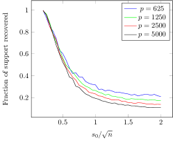
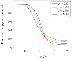
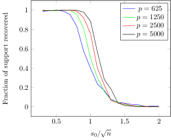
Figure 1: The support recovery phase transitions for Diagonal Thresholding (left) and Covariance Thresholding (center) and the data-driven version of Section 4 (right). For Covariance Thresholding, the fraction of support recovered correctly increases monotonically with $p$, as long as $s_{0}\leq c\sqrt{n}$ with $c\approx 1.1$. Further, it appears to converge to one throughout this region. For Diagonal Thresholding, the fraction of support recovered correctly decreases monotonically with $p$ for all $s_{0}$ of order $\sqrt{n}$. This confirms that Covariance Thresholding (with or without knowledge of the support size $s_{0}$) succeeds with high probability for $s_{0}\leq c\sqrt{n}$, while Diagonal Thresholding requires a significantly sparser principal component.

We plot the empirical success probability as a function of $s_{0}/\sqrt{n}$ for several values of $p$, with $p=n$. The empirical success probability was computed by using $100$ independent instances of the problem. A few observations are of interest: $(i)$ Covariance Thresholding appears to have a significantly larger success probability in the ‘difficult’ regime where Diagonal Thresholding starts to fail; $(ii)$ The curves for Diagonal Thresholding appear to decrease monotonically with $p$ indicating that $s_{0}$ proportional to $\sqrt{n}$ is not the right scaling for this algorithm (as is known from theory); $(iii)$ In contrast, the curves for Covariance Thresholding become steeper for larger $p$, and, in particular, the success probability increases with $p$ for $s_{0}\leq 1.1\sqrt{n}$. This indicates a sharp threshold for $s_{0}={\rm const}\cdot\sqrt{n}$, as suggested by our theory.

In terms of practical applicability, our algorithm in Table 1 has the shortcomings of requiring knowledge of problem parameters $s_{0},\beta,\theta$. Furthermore, the thresholds $\rho,\tau$ suggested by theory need not be optimal. We next describe a principled approach to estimating (where possible) the parameters of interest and running the algorithm in a purely data-dependent manner. Assume the following model, for $i\in[n]$

$${\mathbf{x}}_{i} ={\boldsymbol{\mu}}+\sum_{q}\sqrt{\beta_{q}}u_{q,i}{\mathbf{v}}_{q}+\sigma{\mathbf{z}}_{i},$$

where ${\boldsymbol{\mu}}\in\mathbb{R}^{p}$ is a fixed mean vector, $u_{q,i}$ have mean $0$ and variance $1$, and ${\mathbf{z}}_{i}$ have mean $0$ and covariance ${\rm I}_{p}$. Note that our focus in this section is not on rigorous analysis, but instead to demonstrate a principled approach to applying covariance thresholding in practice. We proceed as follows:

Estimating ${\boldsymbol{\mu}}$, $\sigma$:

We let $\widehat{\boldsymbol{\mu}}=\sum_{i=1}^{n}{\mathbf{x}}_{i}/n$ be the empirical mean estimate for $\mu$. Further letting $\overline{\mathbf{X}}={\mathbf{X}}-\mathbf{1}\widehat{{\boldsymbol{\mu}}}^{\sf T}$ we see that $pn-(\sum_{q}k_{q})n\approx pn$ entries of $\overline{\mathbf{X}}$ are mean $0$ and variance $\sigma^{2}$. We let $\widehat{\sigma}={{\rm MAD}(\overline{\mathbf{X}})}/{\nu}$ where ${\rm MAD}(\,\cdot\,)$ denotes the median absolute deviation of the entries of the matrix in the argument, and $\nu$ is a constant scale factor. Guided by the Gaussian case, we take $\nu=\Phi^{-1}(3/4)\approx 0.6745$.

Choosing $\tau$:

Although in the statement of the theorem, our choice of $\tau$ depends on the SNR $\beta/\sigma^{2}$, it is reasonable to instead threshold ‘at the noise level’, as follows. The noise component of entry $i,j$ of the sample covariance (ignoring lower order terms) is given by $\sigma^{2}\langle{\mathbf{z}}_{i},{\mathbf{z}}_{j}\rangle/n$. By the central limit theorem, $\langle{\mathbf{z}}_{i},{\mathbf{z}}_{j}\rangle/\sqrt{n}{\,\stackrel{{\scriptstyle\mathrm{d}}}{{\Rightarrow}}\,}{\sf N}(0,1)$. Consequently, $\sigma^{2}\langle{\mathbf{z}}_{i},{\mathbf{z}}_{j}\rangle/n\approx{\sf N}(0,\sigma^{4}/n)$, and we need to choose the (rescaled) threshold proportional to $\sqrt{\sigma^{4}}=\sigma^{2}$. Using previous estimates, we let $\tau=\nu^{\prime}\cdot\widehat{\sigma}^{2}$ for a constant $\nu^{\prime}$. In simulations, a choice $3\lesssim\nu^{\prime}\lesssim 4$ appears to work well.

Estimating $r$:

We define ${\mathbf{\widehat{\Sigma}}}=\overline{\mathbf{X}}^{\sf T}\overline{\mathbf{X}}/n-\widehat{\sigma}^{2}{\rm I}_{p}$ and soft threshold it to get $\eta({\mathbf{\widehat{\Sigma}}})$ using $\tau$ as above. Our proof of Theorem 2 relies on the fact that $\eta({\mathbf{\widehat{\Sigma}}})$ has $r$ eigenvalues that are separated from the bulk of the spectrum. Hence, we estimate $r$ using $\widehat{r}$: the number of eigenvalues separated from the bulk in $\eta({\mathbf{\widehat{\Sigma}}})$. The edge of the spectrum can be computed numerically using the Stieltjes transform method as in [CS13].

Estimating ${\mathbf{v}}_{q}$:

Let $\mathbf{\widehat{v}}_{q}$ denote the $q^{\text{th}}$ eigenvector of $\eta({\mathbf{\widehat{\Sigma}}})$. Our theoretical analysis indicates that $\mathbf{\widehat{v}}_{q}$ is expected to be close to ${\mathbf{v}}_{q}$. In order to denoise $\mathbf{\widehat{v}}_{q}$, we assume ${\mathbf{\widehat{\Sigma}}}\mathbf{\widehat{v}}_{q}\approx(1-\delta){\mathbf{v}}_{q}+{\boldsymbol{{\varepsilon}}}_{q}$, where ${\boldsymbol{{\varepsilon}}}_{q}$ is additive random noise (perhaps with some sparse corruptions). We then threshold ${\mathbf{\widehat{\Sigma}}}{\mathbf{v}}_{q}$ ‘at the noise level’ to recover a better estimate of ${\mathbf{v}}_{q}$. To do this, we estimate the standard deviation of the “noise” ${\boldsymbol{{\varepsilon}}}$ by $\widehat{\sigma_{{\boldsymbol{{\varepsilon}}}}}={{\rm MAD}(\mathbf{\widehat{v}}_{q})}/{\nu}$. Here we set –again guided by the Gaussian heuristic– $\nu\approx 0.6745$. Since ${\mathbf{v}}_{q}$ is sparse, this procedure returns a good estimate for the size of the noise deviation. We let $\mathbf{\widehat{v}}^{\prime}_{q}$ denote the vector obtained by hard thresholding $\mathbf{\widehat{v}}_{q}$: set $\mathbf{\widehat{v}}^{\prime}_{i}=\mathbf{\widehat{v}}_{q,i}\text{ if }\lvert{\widehat{v}_{q,i}}\rvert\geq\nu^{\prime}\widehat{\sigma}_{{\boldsymbol{{\varepsilon}}}_{q}}$ and $0\text{ otherwise.}$ We then let $\mathbf{\widehat{v}}^{*}_{q}=\mathbf{\widehat{v}}^{\prime}_{q}/\lVert{\mathbf{\widehat{v}}^{\prime}_{q}}\rVert$ and return $\mathbf{\widehat{v}}^{*}_{q}$ as our estimate for ${\mathbf{v}}_{q}$.

Note that –while different in several respects– this empirical approach shares the same philosophy of the algorithm in Table 1. On the other hand, the data-driven algorithm presented in this section is less straightforward to analyze, a task that we defer to future work.

Figure 1 also shows results of a support recovery experiment using the ‘data-driven’ version of this section. Covariance thresholding in this form also appears to work for supports of size $s_{0}\leq\text{const}\sqrt{n}$. Figure 2 shows the performance of vanilla PCA, Diagonal Thresholding and Covariance Thresholding on the “Three Peak” example of [JL04]. This signal is sparse in the wavelet domain and the simulations employ the data-driven version of covariance thresholding. A similar experiment with the “box” example of Johnstone and Lu is provided in Figure 3. These experiments demonstrate that, while for large values of $n$ both Diagonal Thresholding and Covariance Thresholding perform well, the latter appears superior for smaller values of $n$.

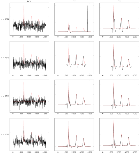
Figure 2: The results of Simple PCA, Diagonal Thresholding and Covariance Thresholding (respectively) for the “Three Peak” example of [JL09] (see Figure 1 of the paper). The signal is sparse in the ‘Symmlet 8’ basis. We use $\beta=1.4,p=4096$, and the rows correspond to sample sizes $n=1024,1625,2580,4096$ respectively. Parameters for Covariance Thresholding are chosen as in Section 4, with $\nu^{\prime}=4.5$. Parameters for Diagonal Thresholding are from [JL09]. On each curve, we superpose the clean signal (dotted).

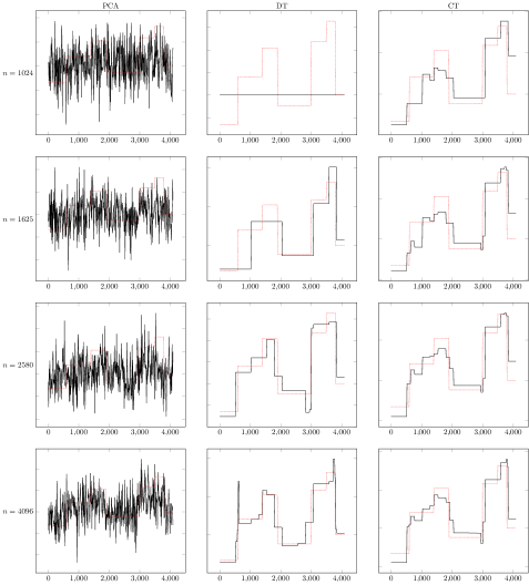
Figure 3: The results of Simple PCA, Diagonal Thresholding and Covariance Thresholding (respectively) for a synthetic block-constant function (which is sparse in the Haar wavelet basis). We use $\beta=1.4,p=4096$, and the rows correspond to sample sizes $n=1024,1625,2580,4096$ respectively. Parameters for Covariance Thresholding are chosen as in Section 4, with $\nu^{\prime}=4.5$. Parameters for Diagonal Thresholding are from [JL09]. On each curve, we superpose the clean signal (dotted).

5 Proof preliminaries

In this section we review some notation and preliminary facts that we will use throughout the paper.

5.1 Notation

We let $[m]=\{1,2,\dots,m\}$ denote the set of first $m$ integers. We will represent vectors using boldface lower case letters, e.g. ${\mathbf{u}},{\mathbf{v}},{\mathbf{x}}$. The entries of a vector ${\mathbf{u}}\in\mathbb{R}^{n}$ will be represented by $u_{i},i\in[n]$. Matrices are represented using boldface upper case letters e.g. ${\mathbf{A}},{\mathbf{X}}$. The entries of a matrix ${\mathbf{A}}\in\mathbb{R}^{m\times n}$ are represented by ${\mathbf{A}}_{ij}$ for $i\in[m],j\in[n]$. Given a matrix ${\mathbf{A}}\in\mathbb{R}^{m\times n}$, we generically let ${\mathbf{a}}_{1}$, ${\mathbf{a}}_{2},\dots,{\mathbf{a}}_{m}$ denote its rows, and ${\mathbf{\tilde{a}}}_{1}$, ${\mathbf{\tilde{a}}}_{2},\dots,{\mathbf{\tilde{a}}}_{n}$ its columns.

For $E\subseteq[m]\times[n]$, we define the projector operator ${\cal P}_{E}:\mathbb{R}^{m\times n}\to\mathbb{R}^{m\times n}$ by letting ${\cal P}_{E}({\mathbf{A}})$ be the matrix with entries

$${\cal P}_{E}({\mathbf{A}})_{ij}=\begin{cases}{\mathbf{A}}_{ij}&\mbox{if $(i,j)\in E$,}\\ 0&\mbox{otherwise.}\end{cases}$$ (23)

For a matrix ${\mathbf{A}}\in\mathbb{R}^{m\times n}$, and a set $E\subseteq[n]$, we define its column restriction ${\mathbf{A}}_{E}\in\mathbb{R}^{m\times n}$ to be the matrix obtained by setting to $0$ columns outside $E$:

$$({\mathbf{A}}_{E})_{ij} =\begin{cases}{\mathbf{A}}_{ij}&\text{ if }j\in E,\\ 0&\text{otherwise. }\end{cases}$$

Similarly ${\mathbf{y}}_{E}$ is obtained from ${\mathbf{y}}$ by setting to zero all indices outside $E$. The operator norm of a matrix ${\mathbf{A}}$ is denoted by $\lVert{{\mathbf{A}}}\rVert$ (or $\lVert{{\mathbf{A}}}\rVert_{op}$) and its Frobenius norm by $\lVert{{\mathbf{A}}}\rVert_{F}$. We write $\lVert{{\mathbf{x}}}\rVert$ for the standard $\ell_{2}$ norm of a vector ${\mathbf{x}}$. Other vector norms such as $\ell_{1}$ or $\ell_{\infty}$ are denoted with appropriate subscripts.

We let ${\sf Q}_{q}$ denotes the support of the $q^{\text{th}}$ spike ${\mathbf{v}}_{q}$. Also, we denote the union of the supports of ${\mathbf{v}}_{q}$ by ${\sf Q}=\cup_{q}{\sf Q}_{q}$. The complement of a set $E\in[n]$ is denoted by $E^{c}$.

We write $\eta(\cdot;\cdot)$ for the soft-thresholding function. By $\partial\eta(\cdot;\tau)$ we denote the derivative of $\eta(\cdot;\tau)$ with respect to the first argument, which exists Lebesgue almost everywhere. To simplify the notation, we omit the second argument when it is understood from context.

For a random variable $Z$ and a measurable set ${\cal A}$ we write ${\mathbb{E}}\{Z;{\cal A}\}$ to denote ${\mathbb{E}}\{Z\mathbb{I}(Z\in{\cal A})\}$, the expectation of $Z$ constrained to the event ${\cal A}$.

In the statements of our results, consider the limit of large $p$ and large $n$ with certain conditions on $p,n$ (as in Theorem 1). This limit will be referred to either as “$n$ large enough” or “$p$ large enough” where the phrase “large enough” indicates dependence of $p$ (and thereby $n$) on specific problem parameters.

The Gaussian distribution function will be denoted by $\Phi(x)=\int_{-\infty}^{x}e^{-t^{2}/2}\,{\rm d}t/\sqrt{2\pi}$.

5.2 Preliminary facts

Let ${\mathbb{S}}^{N-1}$ denote the unit sphere in $N$ dimensions, i.e. ${\mathbb{S}}^{N-1}=\{{\mathbf{x}}\in\mathbb{R}^{N}:\lVert{{\mathbf{x}}}\rVert=1\}$. We use the following definition [Ver12, Definition 5.2] of the ${\varepsilon}$-net of a set $X\subseteq\mathbb{R}^{n}$:

Definition 5.1 (Nets, Covering numbers).

A subset $T^{\varepsilon}(X)\subseteq X$ is called an ${\varepsilon}$-net of $X$ if every point in $X$ may be approximated by one in $T^{\varepsilon}(X)$ with error at most ${\varepsilon}$. More precisely:

$$\forall x\in X,\quad\inf_{y\in T^{\varepsilon}(X)}\lVert{x-y}\rVert \leq{\varepsilon}.$$

The minimum cardinality of an ${\varepsilon}$-net of $X$, if finite, is called its covering number.

The following two facts are useful while using ${\varepsilon}$-nets to bound the spectral norm of a matrix. For proofs, we refer the reader to [Ver12, Lemmas 5.2, 5.4].

Lemma 5.2.

Let $S^{n-1}$ be the unit sphere in $n$ dimensions. Then there exists an ${\varepsilon}$-net of $S^{n-1}$, $T^{\varepsilon}(S^{n-1})$ satisfying:

$$|T^{\varepsilon}(S^{n-1})|\leq\left(1+\frac{2}{{\varepsilon}}\right)^{n}.$$

Lemma 5.3.

Let ${\mathbf{A}}\in\mathbb{R}^{n\times n}$ be a symmetric matrix. Then, there exists ${\mathbf{x}}\in T^{{\varepsilon}}(S^{n-1})$ such that

$$\lvert{\langle{\mathbf{x}},{\mathbf{A}}{\mathbf{x}}\rangle}\rvert \geq(1-2{\varepsilon})\lVert{\mathbf{A}}\rVert.$$ (24)

Proof.

Firstly, we have $\lVert{A}\rVert=\max_{{\mathbf{x}}\in{\mathbb{S}}^{n-1}}\lvert{\langle{\mathbf{x}},{\mathbf{A}}{\mathbf{x}}\rangle}\rvert=\max_{{\mathbf{x}}\in{\mathbb{S}}^{n-1}}\lVert{{\mathbf{A}}{\mathbf{x}}}\rVert$. Let ${\mathbf{x}}_{*}$ be the maximizer (which exists as ${\mathbb{S}}^{n-1}$ is compact and $|\langle{\mathbf{x}},{\mathbf{A}}{\mathbf{x}}\rangle|$ is continuous in ${\mathbf{x}}$). Choose ${\mathbf{x}}\in T^{\varepsilon}_{n}$ so that $\lVert{{\mathbf{x}}-{\mathbf{x}}_{*}}\rVert\leq{\varepsilon}$. Then:

$$\langle{\mathbf{x}},{\mathbf{A}}{\mathbf{x}}\rangle =\langle{\mathbf{x}}-{\mathbf{x}}_{*},{\mathbf{A}}({\mathbf{x}}+{\mathbf{x}}_{*})\rangle+\langle{\mathbf{x}}_{*},{\mathbf{A}}{\mathbf{x}}_{*}\rangle\,.$$ (25)

The lemma then follows as $\lvert{\langle{\mathbf{x}},{\mathbf{A}}({\mathbf{x}}-{\mathbf{x}}_{*})\rangle}\rvert\leq\lVert{{\mathbf{x}}+{\mathbf{x}}_{*}}\rVert\lVert{{\mathbf{A}}}\rVert\lVert{{\mathbf{x}}-{\mathbf{x}}_{*}}\rVert\leq 2{\varepsilon}\lVert{{\mathbf{A}}}\rVert$. ∎

Throughout the paper we will denote by $T^{\varepsilon}_{N}$ an ${\varepsilon}$-net on the unit sphere ${\mathbb{S}}^{N-1}$ that satisfies Lemma 5.2. For a subset of indices ${\sf S}\subset[N]$ we denote by $T^{\varepsilon}_{N}({\sf S})$ the natural isometric embedding of $T^{\varepsilon}_{{\sf S}}$ in ${\mathbb{S}}^{N-1}$.

We now state a general concentration lemma. This will be our basic tool to establish Theorem 2, and thereby Theorem 3.

Lemma 5.4.

Let ${\mathbf{z}}\sim{\sf N}(0,{\rm I}_{N})$ be vector of $N$ i.i.d. standard normal variables. Suppose $S$ is a finite set and we have functions $F_{s}:\mathbb{R}^{N}\to\mathbb{R}$ for every $s\in S$. Assume $\mathcal{G}\in\mathbb{R}^{N}\times\mathbb{R}^{N}$ is a Borel set such that for Lebesgue-almost every $({\mathbf{x}},{\mathbf{y}})\in\mathcal{G}$:

$$\max_{s\in S}\max_{t\in[0,1]}\lVert{{\nabla}F_{s}(\sqrt{t}{\mathbf{x}}+\sqrt{1-t}{\mathbf{y}})}\rVert \leq L\,.$$ (26)

Then, for any $\Delta>0$:

$${\mathbb{P}}\Big{\{}\max_{s\in S}\lvert{F_{s}({\mathbf{z}})-{\mathbb{E}}F_{s}({\mathbf{z}})}\rvert\geq\Delta\Big{\}} \leq C\lvert{S}\rvert\,\exp\Big{(}-\frac{\Delta^{2}}{CL^{2}}\Big{)}+\frac{C}{\Delta^{2}}{\mathbb{E}}\Big{\{}\max_{s\in S}\big{[}(F_{s}({\mathbf{z}})-F_{s}({\mathbf{z}}^{\prime}))^{2}\big{]};\mathcal{G}^{c}\Big{\}}.$$ (27)

Here ${\mathbf{z}}^{\prime}$ is an independent copy of ${\mathbf{z}}$.

Proof.

We use the Maurey-Pisier method along with symmetrization. By centering, assume that ${\mathbb{E}}F_{s}({\mathbf{z}})=0$ for all $s\in S$. Further, by including the functions $-F_{s}$ in the set $S$ (at most doubling its size), it suffices to prove the one-sided version of the inequality:

$${\mathbb{P}}\{\max_{s\in S}F_{s}({\mathbf{z}})\geq\Delta\} \leq C\lvert{S}\rvert\,\exp\Big{(}-\frac{\Delta^{2}}{CL^{2}}\Big{)}+\frac{C}{\Delta^{2}}{\mathbb{E}}\{\max_{s}(F_{s}({\mathbf{z}})-F_{s}({\mathbf{z}}^{\prime}))^{2};\mathcal{G}^{c}\}\,.$$ (28)

We first implement the symmetrization. Note that:

$$\{{\mathbf{x}}:\max_{s}F_{s}({\mathbf{x}})\geq\Delta\} \subseteq\{{\mathbf{x}}:\max_{x\in\mathbb{R},s\in S}[2xF_{s}({\mathbf{x}})-x^{2}]\geq\Delta^{2}\}$$ (29)

$$\{{\mathbf{x}},{\mathbf{y}}:\max_{s}[F_{s}({\mathbf{x}})-F_{s}({\mathbf{y}})]\geq\Delta\} \subseteq\{{\mathbf{x}},{\mathbf{y}}:\max_{x\in\mathbb{R},s\in S}[2x(F_{s}({\mathbf{x}})-F_{s}({\mathbf{y}}))-x^{2}]\geq\Delta^{2}\}.$$ (30)

Furthermore, by centering, $F_{s}({\mathbf{z}})={\mathbb{E}}\{F_{s}({\mathbf{z}})-F_{s}({\mathbf{z}}^{\prime})|{\mathbf{z}}\}$. Hence for any non-decreasing convex function $\phi(z)$:

$${\mathbb{E}}\Big{\{}\phi\big{(}\max_{x,s}[2xF_{s}({\mathbf{z}})-x^{2}]\big{)}\Big{\}} \leq{\mathbb{E}}\bigg{\{}\phi\Big{(}\max_{x,s}\big{[}{\mathbb{E}}\{2xF_{s}({\mathbf{z}})-2xF_{s}({\mathbf{z}}^{\prime})-x^{2}|{\mathbf{z}}\}\big{]}\Big{)}\bigg{\}}$$ (31)

$$\stackrel{{\scriptstyle(a)}}{{\leq}}{\mathbb{E}}\bigg{\{}\phi\Big{(}{\mathbb{E}}\big{\{}\max_{x,s}[2x(F_{s}({\mathbf{z}})-F_{s}({\mathbf{z}}^{\prime}))-x^{2}]|{\mathbf{z}}\big{\}}\Big{)}\bigg{\}}$$ (32)

$$\stackrel{{\scriptstyle(b)}}{{\leq}}{\mathbb{E}}\Big{\{}\phi\big{(}\max_{x,s}[2x(F_{s}({\mathbf{z}})-F_{s}({\mathbf{z}}^{\prime}))-x^{2}]\big{)}\Big{\}}.$$ (33)

Here we use Jensen’s inequality with the monotonicity of $\phi(\cdot)$ to obtain $(a)$ and with the convexity of $\phi(\cdot)$ to obtain $(b)$.

Now we choose $\phi(z)=(z-a)_{+}$, for $a=\Delta^{2}/2$.

$${\mathbb{P}}\{\max_{s}F_{s}({\mathbf{z}})\geq\Delta\} \leq{\mathbb{P}}\big{\{}\max_{x,s}[2xF_{s}({\mathbf{z}})-x^{2}]\geq\Delta^{2}\big{\}}$$ (34)

$$\stackrel{{\scriptstyle(a)}}{{\leq}}\phi(\Delta^{2})^{-1}{\mathbb{E}}\Big{\{}\phi\big{(}\max_{x,s}[2xF_{s}({\mathbf{z}})-x^{2}]\big{)}\Big{\}}$$ (35)

$$\stackrel{{\scriptstyle(b)}}{{\leq}}\phi(\Delta^{2})^{-1}{\mathbb{E}}\Big{\{}\phi\big{(}\max_{x,s}[2x(F_{s}({\mathbf{z}})-F_{s}({\mathbf{z}}^{\prime}))-x^{2}]\big{)}\Big{\}}$$ (36)

$$=\phi(\Delta^{2})^{-1}{\mathbb{E}}\Big{\{}\phi\big{(}\max_{s}[(F_{s}({\mathbf{z}})-F_{s}({\mathbf{z}}^{\prime}))^{2}]\big{)}\Big{\}}$$ (37)

$$=\phi(\Delta^{2})^{-1}\bigg{(}{\mathbb{E}}\Big{\{}\phi\big{(}\max_{s}[(F_{s}({\mathbf{z}})-F_{s}({\mathbf{z}}^{\prime}))^{2}]\big{)};\mathcal{G}\Big{\}}$$

$$\quad+{\mathbb{E}}\Big{(}\big{\{}\phi(\max_{s}[(F_{s}({\mathbf{z}})-F_{s}({\mathbf{z}}^{\prime}))^{2}];\mathcal{G}^{c}\big{\}}\Big{)}\,.$$ (38)

Here $(a)$ is Markov’s inequality, and $(b)$ is the symmetrization bound Eq. (33), where we use the fact that $\phi(z)=(z-a)_{+}$ is non-decreasing and convex in $z$.

At this point, it is easy to see that the lemma follows if we are able to control the first term in Eq. (38). We establish this via the Maurey-Pisier method. Define the path ${\mathbf{z}}(\theta)\equiv{\mathbf{z}}\sin\theta+{\mathbf{z}}^{\prime}\cos\theta$, the velocity ${\dot{\mathbf{z}}}\equiv{\mathrm{d}}{\mathbf{z}}/{\mathrm{d}}\theta={\mathbf{z}}\cos\theta-{\mathbf{z}}^{\prime}\sin\theta$.

$${\mathbb{E}}\Big{\{}\phi\big{(}\max_{s}[(F_{s}({\mathbf{z}})-F_{s}({\mathbf{z}}^{\prime}))^{2}]\big{)};\mathcal{G}\Big{\}} =\int_{0}^{\infty}{\mathbb{P}}\Big{\{}\big{(}\max_{s}[(F_{s}({\mathbf{z}})-F_{s}({\mathbf{z}}^{\prime}))^{2}]-a\big{)}_{+}\mathbb{I}(\mathcal{G})\geq x\Big{\}}{\mathrm{d}}x$$ (39)

$$=\int_{0}^{\infty}{\mathbb{P}}\big{\{}\max_{s}[\lvert{F_{s}({\mathbf{z}})-F_{s}({\mathbf{z}}^{\prime})}\rvert]\geq\sqrt{x+a};\mathcal{G}\big{\}}{\mathrm{d}}x$$ (40)

$$\leq 2|S|\int_{a}^{\infty}e^{-\lambda\sqrt{x}}\max_{s}\Big{[}{\mathbb{E}}\big{\{}\exp\{\lambda(F_{s}({\mathbf{z}})-F_{s}({\mathbf{z}}^{\prime}))\};\mathcal{G}\big{\}}\Big{]}{\mathrm{d}}x\,,$$ (41)

where, in the last inequality we use the union bound followed by Markov’s inequality. To control the exponential moment, note that $F_{s}({\mathbf{z}})-F_{s}({\mathbf{z}}^{\prime})=\int_{0}^{\pi/2}\langle{\nabla}F({\mathbf{z}}(\theta)),{\dot{\mathbf{z}}}(\theta)\rangle{\mathrm{d}}\theta$ whence, using Jensen’s inequality:

$${\mathbb{E}}\Big{\{}\exp\big{\{}\lambda(F_{s}({\mathbf{z}})-F_{s}({\mathbf{z}}^{\prime}))\big{\}};\mathcal{G}\Big{\}} ={\mathbb{E}}\bigg{\{}\exp\Big{(}\int_{0}^{\pi/2}\lambda\langle{\nabla}F_{s}({\mathbf{z}}(\theta)),{\dot{\mathbf{z}}}(\theta)\rangle{\mathrm{d}}\theta\Big{)};\mathcal{G}\bigg{\}}$$ (42)

$$\leq\frac{2}{\pi}\int_{0}^{\pi/2}{\mathbb{E}}\Big{\{}\exp\big{(}\lambda\pi\langle{\nabla}F_{s}({\mathbf{z}}(\theta)),{\dot{\mathbf{z}}}(\theta)\rangle/2\big{)};\mathcal{G}\Big{\}}{\mathrm{d}}\theta.$$ (43)

Define the set $\mathcal{G}_{\theta}=\{({\mathbf{z}},{\mathbf{z}}^{\prime}):\max_{s}\lVert{{\nabla}F_{s}({\mathbf{z}}(\theta))}\rVert\leq L\}$. Then:

$${\mathbb{E}}\Big{\{}\exp\big{\{}\lambda(F_{s}({\mathbf{z}})-F_{s}({\mathbf{z}}^{\prime}))\big{\}};\mathcal{G}\Big{\}} \stackrel{{\scriptstyle(a)}}{{\leq}}\frac{2}{\pi}\int_{0}^{\pi/2}{\mathbb{E}}\Big{\{}\exp\big{(}\lambda\pi\langle{\nabla}F_{s}({\mathbf{z}}(\theta)),{\dot{\mathbf{z}}}(\theta)\rangle/2\big{)};\mathcal{G}_{\theta}\Big{\}}{\mathrm{d}}\theta$$ (44)

$$\stackrel{{\scriptstyle(b)}}{{=}}\frac{2}{\pi}\int_{0}^{\pi/2}{\mathbb{E}}\bigg{\{}\exp\Big{(}\frac{\lambda^{2}\pi^{2}\lVert{{\nabla}F_{s}({\mathbf{z}}(\theta))}\rVert^{2}}{8};\mathcal{G}_{\theta}\Big{)}\bigg{\}}{\mathrm{d}}\theta$$ (45)

$$\stackrel{{\scriptstyle(c)}}{{\leq}}\exp\Big{(}\frac{\lambda^{2}\pi^{2}L^{2}}{8}\Big{)}.$$ (46)

Here $(a)$ follows as $\mathcal{G}_{\theta}\supseteq\mathcal{G}$. Equality $(b)$ follows from noting that $\mathcal{G}_{\theta}$ is measurable with respect to ${\mathbf{z}}(\theta)$ and, hence, first integrating with respect to ${\dot{\mathbf{z}}}(\theta)={\mathbf{z}}\cos\theta-{\mathbf{z}}^{\prime}\sin\theta$, a Gaussian random variable that is independent of ${\mathbf{z}}(\theta)$. The final inequality $(c)$ follows by using the fact that $\lVert{{\nabla}F_{s}({\mathbf{z}}(\theta))}\rVert\leq L$ on the set $\mathcal{G}_{\theta}$.

Since this bound is uniform over $s\in S$, we can use it in (41):

$${\mathbb{E}}\left\{\phi(\max_{s}(F_{s}({\mathbf{z}})-F_{s}({\mathbf{z}}^{\prime}))^{2});\mathcal{G}\right\} \leq 2|S|\int_{a}^{\infty}\exp\Big{(}-\lambda\sqrt{x}+\frac{\lambda^{2}\pi^{2}L^{2}}{8}\Big{)}{\mathrm{d}}x$$ (47)

$$\leq\frac{4|S|}{\lambda^{2}}(1+\lambda\sqrt{a})\exp\Big{(}-\lambda\sqrt{a}+\frac{\lambda^{2}\pi^{2}L^{2}}{8}\Big{)}$$ (48)

We can now set $\lambda=4\sqrt{a}/\pi^{2}L^{2}$, to obtain the exponent above as $-2a/\pi^{2}L^{2}=-\Delta^{2}/\pi^{2}L^{2}$. The prefactor $(1+\lambda\sqrt{a})\lambda^{-2}$ is bounded by $CL^{2}\max(,L^{2}/\Delta^{2})$ when $a=\Delta^{2}/2$. Therefore, as required, we obtain:

$${\mathbb{E}}\left\{\phi(\max_{s}(F_{s}({\mathbf{z}})-F_{s}({\mathbf{z}}^{\prime}))^{2});\mathcal{G}\right\} \leq C\max(1,L^{4}/\Delta^{4})\exp\Big{(}-\frac{\Delta^{2}}{CL^{2}}\Big{)}$$ (49)

Combining this with Eq. (38) and the fact that $\phi(\Delta^{2})^{-1}\leq C\Delta^{-2}$ gives Eq. (28) and, consequently, the lemma. ∎

By a simple application of Cauchy-Schwarz, this lemma implies the following.

Corollary 5.5.

Under the same conditions as Lemma 5.4,

$${\mathbb{P}}\Big{\{}\max_{s\in S}\lvert{F_{s}({\mathbf{z}})-{\mathbb{E}}F_{s}({\mathbf{z}})}\rvert\geq\Delta\Big{\}} \leq C\lvert{S}\rvert\,\exp\Big{(}-\frac{\Delta^{2}}{CL^{2}}\Big{)}$$

$$\quad+\frac{C}{\Delta^{2}}{\mathbb{E}}\Big{\{}\max_{s\in S}\big{[}(F_{s}({\mathbf{z}})-F_{s}({\mathbf{z}}^{\prime}))^{4}\big{]}\Big{\}}^{1/2}{\mathbb{P}}\{\mathcal{G}^{c}\}^{1/2}.$$ (50)

The following two lemmas are well-known concentration of measure results. The forms below can be found in [Ver12, Corollary 5.35], [LM00, Lemma 1] respectively.

Lemma 5.6.

Let ${\mathbf{A}}\in\mathbb{R}^{M\times N}$ be a matrix with i.i.d. standard normal entries, i.e. ${\mathbf{A}}_{ij}\sim{\sf N}(0,1)$. Then, for every $t\geq 0$:

$${\mathbb{P}}\left\{\lVert{{\mathbf{A}}}\rVert_{op}\geq\sqrt{M}+\sqrt{N}+t\right\} \leq\exp\left(-\frac{t^{2}}{2}\right).$$ (51)

Lemma 5.7.

Let ${\mathbf{z}}\sim{\sf N}(0,{\rm I}_{N})$. Then

$${\mathbb{P}}\{\lVert{{\mathbf{z}}}\rVert^{2}\geq N+2\sqrt{Nt}+2t\} \leq\exp(-t).$$ (52)

6 Proof of Theorem 1

Since ${\mathbf{\widehat{\Sigma}}}={\mathbf{X}}^{{\sf T}}{\mathbf{X}}/n-{\rm I}_{p}$, we have:

$${\mathbf{\widehat{\Sigma}}} =\sum_{q=1}^{r}\left\{\frac{\beta_{q}\lVert{{\mathbf{u}}_{q}}\rVert^{2}}{n}{\mathbf{v}}_{q}({\mathbf{v}}_{q})^{\sf T}+\frac{\sqrt{\beta_{q}}}{n}\big{(}{\mathbf{v}}_{q}({\mathbf{Z}}^{{\sf T}}{\mathbf{u}}_{q})^{\sf T}+({\mathbf{Z}}^{\sf T}{\mathbf{u}}_{q}){\mathbf{v}}_{q}^{\sf T}\big{)}\right\}$$

$$\quad+\sum_{q\neq q^{\prime}}\left\{\frac{\sqrt{\beta_{q}\beta_{q^{\prime}}}\langle{\mathbf{u}}_{q},{\mathbf{u}}_{q^{\prime}}\rangle}{n}{\mathbf{v}}_{q}({\mathbf{v}}_{q^{\prime}})^{\sf T}\right\}+\frac{{\mathbf{Z}}^{\sf T}{\mathbf{Z}}}{n}-{\rm I}_{p}\,.$$ (53)

We let ${\sf D}=\{(i,i):i\in[p]\setminus{\sf Q}\}$ be the diagonal entries not included in any support. (Recall that ${\sf Q}=\cup_{q}{\sf Q}_{q}$ denote the union of the supports.) Further let ${\sf E}={\sf Q}\times{\sf Q}$, ${\sf F}=({\sf Q}^{c}\times{\sf Q}^{c})\backslash{\sf D}$, and ${\sf G}=[p]\times[p]\backslash({\sf D}\cup{\sf E}\cup{\sf F})$, or, equivalently ${\sf G}=({\sf Q}\times{\sf Q}^{c})\cup({\sf Q}^{c}\times{\sf Q})$. Since these are disjoint we have:

$$\eta({\mathbf{\widehat{\Sigma}}}) =\underbrace{{\cal P}_{{\sf E}}\left\{\eta({\mathbf{\widehat{\Sigma}}})\right\}}_{{\mathbf{S}}}+\underbrace{{\cal P}_{{\sf F}}\left\{\eta\left({\mathbf{\widehat{\Sigma}}}\right)\right\}}_{{\mathbf{N}}}+\underbrace{{\cal P}_{{\sf G}}\left\{\eta({\mathbf{\widehat{\Sigma}}})\right\}}_{{\mathbf{C}}}+\underbrace{{\cal P}_{{\sf D}}\left\{\eta({\mathbf{\widehat{\Sigma}}})\right\}}_{{\mathbf{D}}}.$$ (54)

The first term corresponds to the ‘signal’ component, while the last three terms correspond to the ‘noise’ component.

Theorem 1 is a direct consequence of the next five propositions. The first demonstrates that, even for a low level of thresholding, viz. $\tau<\sqrt{\log p}/2$, the term $\mathbf{N}$ has small operator norm. The second demonstrates that the soft thresholding operation preserves the signal in the term $\mathbf{S}$. The next two propositions show that the cross and diagonal terms $\mathbf{C}$ and $\mathbf{D}$ are negligible as well. Finally, in the last proposition, we demonstrate that, for the regime of thresholding far above the noise level, i.e. $\tau>C\sqrt{\log p}$, the noise terms $\mathbf{N}$ and $\mathbf{C}$ vanish entirely.

Proposition 6.1.

Let ${\mathbf{N}}$ denote the second term of Eq. (54). Since ${\sf F}={\sf Q}^{c}\times{\sf Q}^{c}\backslash{\sf D}$,

$${\mathbf{N}} ={\cal P}_{{\sf F}}\left(\eta({\mathbf{\widehat{\Sigma}}})\right)={\cal P}_{{\sf F}}\left\{\eta\left(\frac{1}{n}{\mathbf{Z}}^{\sf T}{\mathbf{Z}}\right)\right\}.$$ (55)

Then, there exists an absolute constant $C$ such that the following happens. Assuming that $(i)$ $\tau<\sqrt{\log p}/2$ and $(ii)$ $n>C\log p$, then with probability $1-o(1)$

$$\lVert{{\mathbf{N}}}\rVert_{op}\leq C\,\left(\sqrt{\frac{p}{n}}\vee\frac{p}{n}\right)\,e^{-\tau^{2}/C}\,.$$ (56)

Proposition 6.2.

Let ${\mathbf{S}}$ denote the first term in Eq. (54):

$${\mathbf{S}} ={\cal P}_{\sf E}\left\{\eta({\mathbf{\widehat{\Sigma}}})\right\}.$$ (57)

Assume that $(i)$ $s_{0}/n<1$ and $(ii)n>C\log p$: Then with probability $1-o(1)$:

$$\big{\|}{\mathbf{S}}-{\mathbf{\Sigma}}\big{\|}_{op}\leq\frac{2\tau s_{0}}{\sqrt{n}}+C(\beta\vee 1)\sqrt{\frac{s_{0}}{n}}\,.$$ (58)

Proposition 6.3.

Let $\mathbf{C}$ denote the matrix corresponding to the third term of Eq. (54):

$${\mathbf{C}} ={\cal P}_{{\sf G}}\left\{\eta({\mathbf{\widehat{\Sigma}}})\right\}.$$

Assuming the conditions of Proposition 6.1 and, additionally, that $s_{0}^{2}\leq p$, there exist constants $C,c$ such that with probability $1-o(1)$

$$\lVert{\mathbf{C}}\rVert_{op} \leq C\,\tau e^{-c\tau^{2}/(\beta\vee 1)}\sqrt{\frac{p}{n}}\vee\frac{p}{n}.$$ (59)

Proposition 6.4.

Let $\mathbf{D}$ denote the matrix corresponding to the third term of Eq. (54):

$$\mathbf{D} ={\cal P}_{{\sf D}}\left\{\eta({\mathbf{\widehat{\Sigma}}})\right\}.$$

With probability $1-o(1)$ we have that $\lVert{\mathbf{D}}\rVert_{op}\leq C\sqrt{n^{-1}\log p}$.

Proposition 6.5.

For some absolute constant $C_{0}$, we have for $\tau\geq C_{0}(\beta\vee 1)\sqrt{\log p}$ that, with probability $1-o(1)$:

$$\forall i,j\quad N_{ij}=C_{ij}=0.$$ (60)

Therefore, $\lVert{\mathbf{N}}\rVert_{op}=0$ and $\lVert{\mathbf{C}}\rVert_{op}=0$.

Remark 6.6.

At this point we remark that the probability $1-o(1)$ can be made quantitative, for e.g. of the form $1-\exp(-\min(\sqrt{p},n)/C_{1})$, for every $n$ large enough. For simplicity of exposition we do not pursue this in the paper.

We defer the proofs of Propositions 6.1, 6.2, 6.3, 6.4 and 6.5 to Sections 6.1, 6.2, 6.3, 6.4 and 6.5 respectively. By combining them for $\beta=O(1)$, we immediately obtain the following bound.

Theorem 4.

There exist numerical constants $C_{0},C_{1}$ such that the following happens. Assume $\beta\leq C_{0}$, $n>C_{1}\log p$ and $\tau\leq\sqrt{\log p}/2$. Then with probability $1-o(1)$:

$$\big{\|}\eta({\mathbf{\widehat{\Sigma}}})-{\mathbf{\Sigma}}\big{\|}_{op} \leq\frac{2\tau s_{0}}{\sqrt{n}}+C\Big{(}\sqrt{\frac{p}{n}}\vee\frac{p}{n}\Big{)}\,e^{-\tau^{2}/C}+C\sqrt{\frac{s_{0}\vee\log p}{n}}\,.$$ (61)

Proof.

The proof is obtained by adding the error terms from Propositions 6.1, 6.2, 6.3 and 6.4, and noting that $\beta$ is bounded. ∎

Using Propositions 6.1, 6.2, 6.3 and 6.4, together with a suitable choice of $\tau$, we obtain the proof of Theorem 1.

Proof of Theorem 1.

Note that in the case $s_{0}^{2}>p/e$ there is no thresholding and hence the result follows from the fact that $\|{\mathbf{\widehat{\Sigma}}}-{\mathbf{\Sigma}}\|_{op}\leq C\sqrt{p/n}$ [Ver12, Remark 5.40].

We assume now that $s_{0}^{2}\leq p/e$ and the case that $\tau_{*}=C_{1}(\beta\vee 1)\sqrt{\log(p/s_{0}^{2})}\leq\sqrt{\log p}/2$. In that case we set $\tau=\tau_{*}\leq\sqrt{\log p}/2$. Below we will keep $C_{1}$ a large enough constant, and check that each of the error terms in Propositions 6.1, 6.2, 6.3 and 6.4 is upper bounded by (a constant times) the right-hand side of Eq. (7). Throughout $C$ will denote a generic constant that can be made as large as we want, and can change from line to line.

We start from Proposition 6.1:

$$\lVert{{\mathbf{N}}}\rVert_{op} \leq C\,\left(\sqrt{\frac{p}{n}}\vee\frac{p}{n}\right)\,\left(\frac{s_{0}^{2}}{p}\right)^{C}$$ (62)

$$\leq C\sqrt{\frac{p}{n}\left(\frac{p}{s_{0}^{2}}\right)^{-C-1}}\;\vee\;C\sqrt{\left(\frac{p}{n}\right)^{2}\left(\frac{p}{s_{0}^{2}}\right)^{-C-2}}$$ (63)

$$\leq C\sqrt{\frac{s_{0}^{2}}{n}\left(\frac{p}{s_{0}^{2}}\right)^{-C}}\;\vee\;C\sqrt{\left(\frac{s_{0}^{2}}{n}\right)^{2}\left(\frac{p}{s_{0}^{2}}\right)^{-C}}$$ (64)

$$\leq C\sqrt{\frac{s_{0}^{2}}{n}\log\frac{p}{s_{0}^{2}}}\,,$$ (65)

where in the last step we used $(e\,s_{0}^{2}/p),(s_{0}^{2}/n)\leq 1$.

Next consider Proposition 6.2:

$$\big{\|}{\mathbf{S}}-{\mathbf{\Sigma}}\big{\|}_{op} \leq C\sqrt{\frac{s_{0}^{2}\tau^{2}}{n}}+C\sqrt{\frac{s_{0}(\beta\vee 1)^{2}}{n}}$$ (66)

$$\leq C\sqrt{\frac{s_{0}^{2}(\beta^{2}\vee 1)}{n}\log\frac{p}{s_{0}^{2}}}\,.$$ (67)

From Proposition 6.3, we get, using the same argument as in Eq. (65)

$$\lVert{\mathbf{C}}\rVert_{op} \leq C\sqrt{\beta\vee 1}\,\bigg{(}\sqrt{\frac{p}{n}}\vee\frac{p}{n}\bigg{)}\,\left(\frac{s_{0}^{2}}{p}\right)^{C}$$ (68)

$$\leq C(\beta\vee 1)\sqrt{\frac{s_{0}^{2}}{n}\log\frac{p}{s_{0}^{2}}}.$$ (69)

Finally, the term of Proposition 6.4 is also bounded as desired using $\log p\leq s_{0}^{2}\log(p/s_{0}^{2})$ (dividing both sides by $p$ and using the fact that $x\mapsto x\log(1/x)$ is increasing).

The case of $\tau_{*}\geq\sqrt{\log p}/2$ is easier. In that case, we can keep $\tau=C_{2}\tau_{*}$ with $C_{2}$ large enough so that $\tau\geq C_{0}(\beta\vee 1)\sqrt{\log p}$ for $C_{0}$ of Proposition 6.5. Then, by Proposition 6.5, we know that $\mathbf{N}=0$ and $\mathbf{C}=0$. Therefore we only need consider the terms $\mathbf{S}-{\mathbf{\Sigma}}$ and $\mathbf{D}$. For these terms we can use Propositions 6.2 and 6.4 respectively and, arguing as in the earlier case $\tau_{*}\leq\sqrt{\log p}$, we obtain the desired result. ∎

6.1 Proof of Proposition 6.1

Define ${\mathbf{\widetilde{N}}}$ as

$${\mathbf{\widetilde{N}}} ={\mathcal{P}_{\sf nd}}\left\{\eta\left(\frac{1}{n}{\mathbf{Z}}^{\sf T}{\mathbf{Z}}\right)\right\}.$$

Since ${\mathbf{N}}$ is a principal submatrix of ${\mathbf{\widetilde{N}}}$, it suffices to prove the same bound for ${\mathbf{\widetilde{N}}}$. Our main tool in the proof will be the concentration lemma 5.4 which we use on multiple occasions. With a view to using the lemma, we let let ${\mathbf{Z}}^{\prime}\in\mathbb{R}^{n\times p}$ denote an independent copy of ${\mathbf{Z}}$, and ${\mathbf{\tilde{z}}}^{\prime}_{i}$ it’s $i^{\text{th}}$ column. The proof relies on two preliminary lemmas. For some $A\geq 1$ (to be chosen later), we first state and prove the following lemma that controls the norm of any principal submatrix of $\mathbf{\tilde{N}}$ of size at most $p/A$.

Lemma 6.7.

Fix any $A\geq 1$. There exists an absolute constants $C,c$ such that:

$${\mathbb{P}}\Big{\{}\max_{{\sf S}\subseteq[p],|{\sf S}|\leq p/A}\|{\cal P}_{{\sf S}\times{\sf S}}(\mathbf{\tilde{N}})\|_{op}\geq\Delta\Big{\}} \leq C\,\exp\Big{(}p\frac{\log CA}{A}-\frac{n^{2}\Delta^{2}}{C(n+p)}\Big{)}+C\frac{(np)^{C}}{\Delta^{2}}\exp(-cn).$$ (70)

Proof.

For any subset ${\sf S}\subset[p]$ recall that $T^{\varepsilon}_{p}({\sf S})$ denotes an ${\varepsilon}$-net of unit vectors in ${\mathbb{S}}^{p-1}$ supported on the subset ${\sf S}$. For simplicity let $T(A)=\cup_{{\sf S}:|{\sf S}|\leq p/A}T^{\varepsilon}_{p}({\sf S})$. It suffices, by Lemma 5.3, to control $\langle\mathbf{y},\mathbf{\tilde{N}}\mathbf{y}\rangle$ on the set $T(A)$. In particular:

$${\mathbb{P}}\Big{\{}\max_{{\sf S}\subseteq[p],|{\sf S}|\leq p/A}\|{\cal P}_{{\sf S}\times{\sf S}}(\mathbf{\tilde{N}})\|_{op}\geq\Delta\Big{\}} \leq{\mathbb{P}}\Big{\{}\max_{\mathbf{y}\in T(A)}|\langle\mathbf{y},\mathbf{\tilde{N}}\mathbf{y}\rangle|\geq\Delta(1-2{\varepsilon})\Big{\}}.$$ (71)

Consider the good set $\mathcal{G}_{1}$ given by:

$$\mathcal{G}_{1} =\{({\mathbf{Z}},{\mathbf{Z}}^{\prime}):\max(\lVert{{\mathbf{Z}}}\rVert,\lVert{{\mathbf{Z}}^{\prime}}\rVert)\leq\sqrt{2}(\sqrt{n}+\sqrt{p}))\}.$$ (72)

To use Lemma 5.4, we need to compute ${\mathbb{E}}\langle\mathbf{y},\mathbf{\tilde{N}}\mathbf{y}\rangle$ and the gradient of $\langle\mathbf{y},\mathbf{\tilde{N}}\mathbf{y}\rangle$ with respect to the underlying random variables ${\mathbf{Z}}$. Since $\eta(\cdot)$ is an odd function the expectation vanishes. To compute the gradient, we let $t\in[0,1]$ and $\mathbf{W}=\sqrt{t}{\mathbf{Z}}+\sqrt{1-t}{\mathbf{Z}}^{\prime}$, and consider $\langle\mathbf{y},\mathbf{\tilde{N}}\mathbf{y}\rangle=\langle\mathbf{y},\eta(\mathbf{W}^{\sf T}\mathbf{W}/n)\mathbf{y}\rangle$ as a function of the $\mathbf{W}$. Taking the gradient with respect to a column $\mathbf{\tilde{w}}_{\ell}$ for $\ell\in{\sf S}$:

$${\nabla}_{\mathbf{\tilde{w}}_{\ell}}\langle\mathbf{y},\mathbf{\tilde{N}}\mathbf{y}\rangle =\frac{y_{\ell}}{n}\sum_{i\neq\ell,i\in{\sf S}}\mathbf{\tilde{w}}_{i}y_{i}\partial\eta(\langle\mathbf{\tilde{w}}_{i},\mathbf{\tilde{w}}_{\ell}\rangle/n)$$ (73)

$$=\frac{y_{\ell}}{n}\mathbf{W}{\boldsymbol{\sigma}},$$ (74)

where

$$\sigma_{i} =\begin{cases}y_{i}\partial\eta(\langle\mathbf{\tilde{w}}_{i},\mathbf{\tilde{w}}_{\ell}\rangle/n)&\text{ if }i\neq\ell,i\in{\sf S}\\ 0&\text{otherwise.}\end{cases}$$ (75)

Since $\lVert{{\boldsymbol{\sigma}}}\rVert\leq\lVert{\mathbf{y}}\rVert=1$, we have that $\lVert{{\nabla}_{\mathbf{\tilde{w}}_{\ell}}\langle\mathbf{y},\mathbf{\tilde{N}}\mathbf{y}\rangle}\rVert^{2}\leq y_{\ell}^{2}\lVert{\mathbf{W}}\rVert^{2}/n^{2}$. Summing over $\ell\in{\sf S}$ we obtain the gradient bound, holding on the good set $\mathcal{G}_{1}$:

$$\lVert{{\nabla}_{\mathbf{W}}\langle\mathbf{y},\mathbf{\tilde{N}}\mathbf{y}\rangle}\rVert^{2} \leq\frac{\sum_{\ell}y_{\ell}^{2}}{n^{2}}\lVert{\mathbf{W}}\rVert^{2}$$ (76)

$$\leq\frac{C(n+p)}{n^{2}}\,,$$ (77)

which holds because of triangle inequality and the fact that $\sqrt{t}+\sqrt{1-t}\leq\sqrt{2}$. We can now apply Lemma 5.4 to bound the RHS of Eq. (71) and get:

$${\mathbb{P}}\Big{\{}\max_{{\sf S}\subseteq[p],|{\sf S}|\leq p/A}{\cal P}_{{\sf S}\times{\sf S}}(\mathbf{\tilde{N}})\geq\Delta\Big{\}} \leq C\lvert{T(A)}\rvert\,\exp\Big{(}-\frac{n^{2}\Delta^{2}}{C(n+p)}\Big{)}$$

$$\quad+\frac{C}{\Delta^{2}}{\mathbb{E}}\big{\{}\max_{{\mathbf{y}}\in T}\langle\mathbf{y},\mathbf{\tilde{N}}\mathbf{y}\rangle^{2};\mathcal{G}_{1}^{c}\big{\}}.$$ (78)

We can simplify the terms on the right-hand side to obtain the result of the lemma. With ${\varepsilon}=1/4$, Stirling’s approximation and Lemma 5.2 we have:

$$\lvert{T(A)}\rvert \leq\exp\Big{(}p\frac{\log CA}{A}\Big{)}.$$ (79)

We use a crude bound on the complement of the good set $\mathcal{G}_{1}$. It is easy to see that, for any unit vector ${\mathbf{y}}$, $\langle\mathbf{y},\mathbf{\tilde{N}}\mathbf{y}\rangle^{2}\leq\lVert{\mathbf{\tilde{N}}}\rVert_{F}^{2}\leq\lVert{\mathbf{Z}^{\sf T}\mathbf{Z}}\rVert_{F}^{2}/n^{2}$. Cauchy-Schwarz then implies that

$${\mathbb{E}}\{\max\langle\mathbf{y},\mathbf{\tilde{N}}\mathbf{y}\rangle^{2};\mathcal{G}_{1}^{c}\} \leq n^{-2}\big{(}{\mathbb{E}}\{\lVert{{\mathbf{Z}}^{\sf T}{\mathbf{Z}}}\rVert_{F}^{4}\}\big{)}^{1/2}{\mathbb{P}}\{\mathcal{G}_{1}^{c}\}^{1/2}$$ (80)

$$\leq(np)^{C}\exp(-c(n+p)),$$ (81)

where the bound on ${\mathbb{P}}\{\mathcal{G}_{1}^{c}\}$ follows from Lemma 5.6. This concludes the lemma. ∎

Note that Lemma 6.7, with $A=1$, tells us that $\lVert{\mathbf{\tilde{N}}}\rVert_{op}$ is of order $\sqrt{p/n+(p/n)^{2}}$ (uniformly in $\tau$) with high probability. Already this non-asymptotic bound is non-trivial, since the previous results of [CS13] and [FM15] do not extend to this case. However, Proposition 6.1 is stronger, and establishes a rate of decay with the thresholding level $\tau$.

The second lemma we require controls the Rayleigh quotient $\langle{\mathbf{y}},\mathbf{\tilde{N}}{\mathbf{y}}\rangle$ when the entries of ${\mathbf{y}}$ are “spread out”.

Lemma 6.8.

Assume that $\tau\leq\sqrt{\log p}/2$. Given $A\geq 1$ and a unit vector ${\mathbf{y}}$, let ${\sf S}=\{i:\lvert{y_{i}}\rvert\leq\sqrt{A/p}\}$ and ${\mathbf{y}}_{{\sf S}},{\mathbf{y}}_{{\sf S}^{c}}$ denote the projections of ${\mathbf{y}}$ onto supports ${\sf S},{\sf S}^{c}$ respectively. We have:

$${\mathbb{P}}\Big{\{}\max_{\mathbf{y}\in T^{1/4}_{p}}\lvert\langle\mathbf{y}_{{\sf S}},\mathbf{\tilde{N}}\mathbf{y}_{{\sf S}}\rangle\rvert\geq\Delta\Big{\}} \leq C\exp\Big{(}-\frac{n^{2}\Delta^{2}}{L_{1}^{2}}+Cp\Big{)}+(np)^{C}\exp\big{(}-c\min(\sqrt{p},n)\big{)},$$ (82)

for any $\Delta\geq L_{1}$ where $L_{1}=C_{1}\sqrt{A\exp(-\tau^{2}/16)(n+p)/n^{2}}$. The same bound holds for ${\mathbb{P}}\big{\{}\max_{{\mathbf{y}}\in T^{1/4}_{p}}|\langle{\mathbf{y}}_{{\sf S}^{c}},\mathbf{\tilde{N}}{\mathbf{y}}_{{\sf S}}\rangle|\geq\Delta\big{\}}$.

Proof.

We first prove the claim for $\langle{\mathbf{y}}_{{\sf S}},{\mathbf{\widetilde{N}}}{\mathbf{y}}_{{\sf S}}\rangle$. Firstly, we have ${\mathbb{E}}\langle\mathbf{y}_{{\sf S}},\mathbf{\tilde{N}}{\mathbf{y}}_{{\sf S}}\rangle=0$. Consider the “good set” $\mathcal{G}_{2}$ of pairs $(\mathbf{W},\mathbf{W^{\prime}})\in\mathbb{R}^{n\times p}\times\mathbb{R}^{n\times p}$ satisfying the conditions:

$$\lVert{\mathbf{W}}\rVert,\lVert{\mathbf{W}^{\prime}}\rVert\leq\sqrt{2}(\sqrt{n}+\sqrt{p})\,,$$ (83)

$$\forall i\in[p],\quad\frac{1}{p}\sum_{j\in[p]\backslash i}|\mathbb{I}(\langle\mathbf{\tilde{w}}_{i},\mathbf{\tilde{w}}_{j}\rangle|\geq\tau\sqrt{n}/2) \leq 2\exp(-\tau^{2}/16)\,,$$ (84)

$$\forall i\in[p],\quad\frac{1}{p}\sum_{j\in[p]\backslash i}|\mathbb{I}(\langle\mathbf{\tilde{w}}^{\prime}_{i},\mathbf{\tilde{w}}^{\prime}_{j}\rangle|\geq\tau\sqrt{n}/2) \leq 2\exp(-\tau^{2}/16)\,,$$ (85)

$$\forall i\in[p],\quad\frac{1}{p}\sum_{j\in[p]}\mathbb{I}(|\langle\mathbf{\tilde{w}}_{i},\mathbf{\tilde{w}}^{\prime}_{j}\rangle|\geq\tau\sqrt{n}/2) \leq 2\exp(-\tau^{2}/16).\,.$$ (86)

Also, for any pair $\mathbf{W},\mathbf{W^{\prime}}\in\mathcal{G}_{2}$, for $\mathbf{W}(t)=\sqrt{t}\mathbf{W}+\sqrt{1-t}\mathbf{W^{\prime}}$ (and its columns $\mathbf{\tilde{w}}(t)_{i}$ defined appropriately) we have:

$$\lVert{\mathbf{W}(t)}\rVert\leq\max_{t}(\sqrt{t}+\sqrt{1-t})(\sqrt{2n}+\sqrt{2p})=2(\sqrt{n}+\sqrt{p}),$$ (87)

$$\forall i\in[p]\quad\frac{1}{p}\sum_{j\in[p]\backslash i}\mathbb{I}(\langle\mathbf{\tilde{w}}(t)_{i},\mathbf{\tilde{w}}(t)_{j}\rangle\geq\tau\sqrt{n})\leq 6\exp(-\tau^{2}/16).$$ (88)

Equation (87) follows by a simple application of triangle inequality and condition (83) defining $\mathcal{G}_{2}$. For inequality (88), expanding the product $\langle\mathbf{\tilde{w}}(t)_{i},\mathbf{\tilde{w}}(t)_{j}\rangle$:

$$\langle\mathbf{\tilde{w}}(t)_{i},\mathbf{\tilde{w}}(t)_{j}\rangle =t\langle\mathbf{\tilde{w}}_{i},\mathbf{\tilde{w}}_{j}\rangle+(1-t)\langle\mathbf{\tilde{w}}^{\prime}_{i},\mathbf{\tilde{w}}^{\prime}_{j}\rangle+\sqrt{t(1-t)}\langle\mathbf{\tilde{w_{i}}},\mathbf{\tilde{w}}^{\prime}_{j}\rangle,$$ (89)

whence, by triangle inequality and $\sqrt{t(1-t)}<1$

$$\mathbb{I}(\lvert{\langle\mathbf{\tilde{w}}(t)_{i},\mathbf{\tilde{w}}(t)_{j}\rangle}\rvert\geq\tau\sqrt{n}) \leq\mathbb{I}(\lvert\langle\mathbf{\tilde{w}}_{i},\mathbf{\tilde{w}}_{j}\rangle\rvert\geq\tau\sqrt{n}/2)+\mathbb{I}(\lvert\langle\mathbf{\tilde{w}}^{\prime}_{i},\mathbf{\tilde{w}}^{\prime}_{j}\rangle\rvert\geq\tau\sqrt{n}/2)$$

$$\quad+\mathbb{I}(\lvert\langle\mathbf{\tilde{w}}_{i},\mathbf{\tilde{w}}^{\prime}_{j}\rangle\rvert\geq\tau\sqrt{n}/2).$$ (90)

The gradient of $\langle{\mathbf{y}}_{{\sf S}},\eta(\mathbf{W}^{\sf T}\mathbf{W}/n){\mathbf{y}}_{{\sf S}}\rangle$ with respect to a column $\mathbf{\tilde{w}}_{\ell}$ of $\mathbf{W}$ is given by:

$${\nabla}_{\mathbf{\tilde{w}}_{\ell}}\langle{\mathbf{y}}_{{\sf S}},\eta(\mathbf{W}^{\sf T}\mathbf{W}/n)\mathbf{y}_{{\sf S}}\rangle =\frac{y_{\ell}}{n}\sum_{j\in{\sf S}\backslash\ell}y_{j}\partial\eta\big{(}\frac{\langle\mathbf{\tilde{w}}_{j},\mathbf{\tilde{w}}_{\ell}\rangle}{n};\frac{\tau}{\sqrt{n}}\big{)}\mathbf{\tilde{w}}_{j}$$ (91)

$$=\frac{y_{\ell}}{n}\mathbf{W}{\boldsymbol{\sigma}},$$ (92)

$$\text{ where }\;\sigma_{i} =\begin{cases}\partial\eta(\langle\mathbf{\tilde{w}}_{i},\mathbf{\tilde{w}}_{\ell}\rangle/n;\tau/\sqrt{n})y_{i}&\text{ when }i\in{\sf S}\backslash\ell\\ 0&\text{ otherwise.}\end{cases}$$ (93)

Therefore

$$\lVert{{\nabla}_{\mathbf{\tilde{w}}_{\ell}}\langle{\mathbf{y}}_{{\sf S}},{\mathbf{\widetilde{N}}}{\mathbf{y}}_{{\sf S}}\rangle}\rVert^{2} \leq\frac{y_{\ell}^{2}}{n^{2}}\lVert{\mathbf{W}}\rVert^{2}\lVert{{\boldsymbol{\sigma}}}\rVert^{2}$$ (94)

$$\leq\frac{y_{\ell}^{2}\lVert{\mathbf{W}}\rVert^{2}}{n^{2}}\sum_{i\neq\ell}(y_{i}\partial\eta(\langle\mathbf{\tilde{w}}_{i},\mathbf{\tilde{w}}_{\ell}\rangle/n))^{2}$$ (95)

$$\stackrel{{\scriptstyle(a)}}{{\leq}}\frac{y_{\ell}^{2}\lVert{\mathbf{W}}\rVert^{2}}{n^{2}}\sum_{i\neq\ell}\frac{A}{p}\mathbb{I}(\lvert{\langle\mathbf{\tilde{w}}_{i},\mathbf{\tilde{w}}_{\ell}\rangle}\rvert\geq\tau\sqrt{n})$$ (96)

$$\stackrel{{\scriptstyle(b)}}{{\leq}}\frac{y_{\ell}^{2}}{n^{2}}C(n+p)A\exp(-\tau^{2}/16)$$ (97)

Here $(a)$ follows from fact that the entries of ${\mathbf{y}}_{{\sf S}}$ are bounded by $\sqrt{A/p}$ and the definition of the soft thresholding function. Inequality $(b)$ follows follows when we set $\mathbf{W}=\mathbf{Z}(t)=\sqrt{t}\mathbf{Z}+\sqrt{1-t}\mathbf{Z}^{\prime}$ and $({\mathbf{Z}},{\mathbf{Z}}^{\prime})\in\mathcal{G}_{2}$. Therefore, summing over $\ell$ we obtain the following bound for the gradient of $\langle{\mathbf{y}}_{{\sf S}},{\mathbf{\widetilde{N}}}{\mathbf{y}}_{{\sf S}}\rangle$

$$\lVert{{\nabla}_{\mathbf{Z}(t)}\langle{\mathbf{y}}_{{\sf S}},{\mathbf{\widetilde{N}}}{\mathbf{y}}_{{\sf S}}\rangle}\rVert^{2} \leq C_{1}\frac{A\exp(-\tau^{2}/16)(n+p)}{n^{2}}\equiv L_{1}^{2}.$$ (98)

We can use now Lemma 5.4, to get, for $L_{1}>0$ as defined above and any $\Delta\geq L_{1}$:

$${\mathbb{P}}\Big{\{}\max_{{\mathbf{y}}\in T^{1/4}_{p}}\langle{\mathbf{y}}_{{\sf S}},{\mathbf{\widetilde{N}}}{\mathbf{y}}_{{\sf S}}\rangle\geq\Delta\Big{\}} \leq C\exp\Big{(}-\frac{\Delta^{2}}{CL_{1}^{2}}+Cp\Big{)}$$

$$\quad+CL_{1}^{-2}{\mathbb{E}}\{\max_{{\mathbf{y}}\in T^{\varepsilon}_{p}}\langle{\mathbf{y}}_{{\sf S}},{\mathbf{\widetilde{N}}}{\mathbf{y}}_{{\sf S}}\rangle^{2};\mathcal{G}_{2}\}$$ (99)

$$\leq C\exp\Big{(}-\frac{\Delta^{2}}{CL_{1}^{2}}+Cp\Big{)}+C(np)^{C}{\mathbb{P}}\{\mathcal{G}_{2}^{c}\}^{1/2},$$ (100)

where the last line follows by Cauchy-Schwarz, as in the proof of Lemma 6.7, and the fact that $L_{1}\geq(np)^{-C_{2}}$ using the upper bound $\tau\leq\sqrt{\log p}/2$.

To obtain the thesis, we need to now bound ${\mathbb{P}}\{\mathcal{G}_{2}^{c}\}$. It suffices to control the failure probability of conditions (83), (84), (85), (86) of the good set $\mathcal{G}_{2}$ individually, and apply the union bound. For $\mathbf{Z},\mathbf{Z^{\prime}}$ independent, $\max(\lVert{{\mathbf{Z}}}\rVert,\lVert{{\mathbf{Z}}^{\prime}}\rVert)\geq\sqrt{2}(\sqrt{n}+\sqrt{p})$ with probability at most $2\exp(-c(n+p))$ by Lemma 5.6. Now consider condition (84) with $i=1$, without loss of generality. First, for any $h>0$ we have:

$${\mathbb{P}}\Big{\{}\frac{1}{p}\sum_{j\neq 1}\mathbb{I}(\lvert{\langle{\mathbf{\tilde{z}}}_{1},{\mathbf{\tilde{z}}}_{j}\rangle}\rvert\geq\tau\sqrt{n}/2)\geq h\Big{\}} \leq{\mathbb{P}}\Big{\{}\frac{1}{p}\sum_{j\neq 1}\mathbb{I}(\lvert{\langle{\mathbf{\tilde{z}}}_{1},{\mathbf{\tilde{z}}}_{j}\rangle}\rvert\geq\tau\sqrt{n}/2)\geq 2h;\lVert{{\mathbf{\tilde{z}}}_{1}}\rVert\leq 2\sqrt{n}\Big{\}}$$

$$\quad+{\mathbb{P}}\big{\{}\lVert{{\mathbf{\tilde{z}}}_{1}}\rVert\geq\sqrt{2n}\big{\}}.$$ (101)

Lemma 5.7 guarantees that the second term is at most $\exp(-cn)$. To control the first term, we note that, conditional on ${\mathbf{\tilde{z}}}_{1}$, $\langle{\mathbf{\tilde{z}}}_{j},{\mathbf{\tilde{z}}}_{1}\rangle,j\neq 1$ are independent Gaussian random variables with variance $\lVert{{\mathbf{\tilde{z}}}_{1}}\rVert^{2}$. Therefore, conditional on ${\mathbf{\tilde{z}}}_{1}$, $\mathbb{I}(|\langle{\mathbf{\tilde{z}}}_{1},{\mathbf{\tilde{z}}}_{j}\rangle|\geq\tau\sqrt{n}/2)$ are independent Bernoulli random variables with success probability $h_{0}=2\Phi\big{(}-\tau\sqrt{n}/(2\lVert{\mathbf{\tilde{z}}_{1}}\rVert)\big{)}$, where $\Phi(\cdot)$ is the Gaussian cumulative distribution function. It follows, by the Chernoff-Hoeffding bound for Bernoulli random variables that

$${\mathbb{P}}\Big{\{}\frac{1}{p}\sum_{j\neq 1}\mathbb{I}(\lvert{\langle{\mathbf{\tilde{z}}}_{1},{\mathbf{\tilde{z}}}_{j}\rangle}\rvert\geq\tau\sqrt{n}/2)\geq h\big{|}{\mathbf{\tilde{z}}}_{1}\Big{\}} \leq\exp\big{(}-p\,D(h\|h_{0})\big{)},$$ (102)

where $D(a\|b)=a\log(a/b)+(1-a)\log[(1-a)/(1-b)]$. Choosing $h=4\Phi(-\tau/(2\sqrt{2}))$, and conditional on $\lVert{\mathbf{\tilde{z}}_{1}}\rVert\leq\sqrt{2n}$, $D(h\|h_{0})\geq ch$ for a constant $c$, implying that

$${\mathbb{P}}\Big{\{}\frac{1}{p}\sum_{j\neq 1}\mathbb{I}(\lvert{\langle{\mathbf{\tilde{z}}}_{1},{\mathbf{\tilde{z}}}_{j}\rangle}\rvert\geq\tau\sqrt{n}/2)\geq h;\lVert{{\mathbf{\tilde{z}}}_{1}}\rVert\leq\sqrt{2n}\Big{\}} \leq\exp(-cph).$$ (103)

By standard bounds $h=4\Phi(-\tau/2\sqrt{2})\leq 2\exp(-\tau^{2}/16)$ and, as $\tau\leq\sqrt{\log p}/2$, $h\geq 1/\sqrt{p}$, we have

$${\mathbb{P}}\Big{\{}\frac{1}{p}\sum_{j\neq 1}\mathbb{I}(\lvert{\langle{\mathbf{\tilde{z}}}_{1},{\mathbf{\tilde{z}}}_{j}\rangle}\rvert\geq\tau\sqrt{n}/2)\geq h;\lVert{{\mathbf{\tilde{z}}}_{1}}\rVert\leq\sqrt{2n}\Big{\}} \leq\exp(-c\sqrt{p}).$$ (104)

Combining this with Eq. (101) we now get:

$${\mathbb{P}}\Big{\{}\frac{1}{p}\sum_{j\neq 1}\mathbb{I}(\lvert{\langle{\mathbf{\tilde{z}}}_{1},{\mathbf{\tilde{z}}}_{j}\rangle}\rvert\geq\tau\sqrt{n}/2)\geq h\Big{\}} \leq 2\exp(-c\min(n,\sqrt{p})).$$ (105)

A similar bound holds for $i\neq 1$ and the other conditions (85) and (86), whence we have by the union bound that ${\mathbb{P}}\{\mathcal{G}_{2}^{c}\}\leq p^{2}\exp(-c\min(\sqrt{p},n))$. This completes the proof of the claim (82).

The proof of the claim for $\langle{\mathbf{y}}_{{\sf S}},\mathbf{\tilde{N}}{\mathbf{y}}_{{\sf S}^{c}}\rangle$ is analogous, so we only sketch the points at which it differs from that of Eq. (82). We use the same good set $\mathcal{G}_{2}$, as defined earlier. Computing the gradient as for $\langle{\mathbf{y}}_{{\sf S}},{\mathbf{\widetilde{N}}}{\mathbf{y}}_{{\sf S}}\rangle$ we obtain:

$${\nabla}_{\mathbf{\tilde{w}}_{\ell}}\langle{\mathbf{y}}_{{\sf S}},{\mathbf{\widetilde{N}}}{\mathbf{y}}_{{\sf S}^{c}}\rangle =\frac{y_{\ell}}{n}\sum_{j\in{\sf S}(\ell)}y_{j}\mathbf{\tilde{w}}_{j}\partial\eta\Big{(}\frac{\langle\mathbf{\tilde{w}}_{j},\mathbf{\tilde{w}}_{\ell}\rangle}{n};\frac{\tau}{\sqrt{n}}\Big{)}.$$ (106)

Here ${\sf S}(\ell)={\sf S}^{c}$ if $\ell\in{\sf S}$ and ${\sf S}$ otherwise. Define the vector ${\boldsymbol{\sigma}}(\ell)\in\mathbb{R}^{p}$ as

$$({\boldsymbol{\sigma}}(\ell))_{j} =\begin{cases}y_{\ell}y_{j}\partial\eta\Big{(}\frac{\langle\mathbf{\tilde{w}}_{j},\mathbf{\tilde{w}}_{\ell}\rangle}{n};\frac{\tau}{\sqrt{n}}\Big{)}&\text{ if }j\in{\sf S}(\ell)\\ 0&\text{ otherwise.}\end{cases}$$ (107)

As before, we have that $\lVert{{\nabla}_{\mathbf{\tilde{w}}_{\ell}}\langle{\mathbf{y}}_{{\sf S}},{\mathbf{\widetilde{N}}}{\mathbf{y}}_{{\sf S}^{c}}\rangle}\rVert=n^{-1}\lVert{\mathbf{W}{\boldsymbol{\sigma}}(\ell)}\rVert\leq n^{-1}\lVert{\mathbf{W}}\rVert\lVert{{\boldsymbol{\sigma}}(\ell)}\rVert$. Therefore, summing over $\ell\in[p]$:

$$\lVert{{\nabla}_{\mathbf{W}}\langle{\mathbf{y}}_{{\sf S}},{\mathbf{\widetilde{N}}}{\mathbf{y}}_{{\sf S}^{c}}\rangle}\rVert^{2} \leq\frac{\lVert{\mathbf{W}}\rVert}{n^{2}}\sum_{\ell\in[p]}\lVert{{\boldsymbol{\sigma}}(\ell)}\rVert^{2}$$ (108)

$$\leq\frac{\lVert{\mathbf{W}}\rVert^{2}}{n^{2}}\sum_{\ell\in[p]}\sum_{j\in{\sf S}(\ell)}y_{\ell}^{2}y_{j}^{2}\partial\eta\Big{(}\frac{\langle\mathbf{\tilde{w}}_{j},\mathbf{\tilde{w}}_{\ell}\rangle}{n};\frac{\tau}{\sqrt{n}}\Big{)}$$ (109)

$$=\frac{2\lVert{\mathbf{W}}\rVert^{2}}{n^{2}}\sum_{\ell\in{\sf S}}\sum_{j\in{\sf S}^{c}}y_{j}^{2}y_{\ell}^{2}\partial\eta\Big{(}\frac{\langle\mathbf{\tilde{w}}_{j},\mathbf{\tilde{w}}_{\ell}\rangle}{n};\frac{\tau}{\sqrt{n}}\Big{)}$$ (110)

$$\leq\frac{2\lVert{\mathbf{W}}\rVert^{2}}{n^{2}}\frac{A}{p}\max_{\ell\in[p]}\sum_{j\neq p}\partial\eta\Big{(}\frac{\langle\mathbf{\tilde{w}}_{j},\mathbf{\tilde{w}}_{\ell}\rangle}{n};\frac{\tau}{\sqrt{n}}\Big{)}.$$ (111)

Under the condition of $\mathcal{G}_{2}$, the gradient also satisfies, when evaluated at $\mathbf{W}={\mathbf{Z}}(t)=\sqrt{t}{\mathbf{Z}}+\sqrt{1-t}{\mathbf{Z}}^{\prime}$:

$$\lVert{{\nabla}_{\mathbf{Z}(t)}\langle{\mathbf{y}}_{{\sf S}},{\mathbf{\widetilde{N}}}{\mathbf{y}}_{{\sf S}^{c}}\rangle}\rVert^{2} \leq\frac{CA\exp(-\tau^{2}/16)(n+p)}{n^{2}}.$$ (112)

The rest of the proof is then the same as before. ∎

Given these lemmas, we can now establish Proposition 6.1.

Proof of Proposition 6.1.

We use a variant of the ${\varepsilon}$-net argument of Lemma 6.7. To bound the probability that $\lVert{\mathbf{\tilde{N}}}\rVert_{op}$ is large, with Lemma 5.3, we obtain:

$${\mathbb{P}}\big{\{}\lVert{\mathbf{\tilde{N}}\rVert_{op}}\geq\Delta\big{\}} \leq{\mathbb{P}}\Big{\{}\max_{{\mathbf{y}}\in T^{{\varepsilon}}_{p}}\lvert{\langle\mathbf{y},\mathbf{\tilde{N}}\mathbf{y}\rangle}\rvert\geq\Delta(1-2{\varepsilon})\Big{\}}.$$ (113)

Let ${\sf S}=\{i:\lvert{y_{i}}\rvert\leq\sqrt{A/p}\}$ for some $A\geq 1$ to be chosen later. Then let ${\mathbf{y}}={\mathbf{y}}_{{\sf S}}+{\mathbf{y}}_{{\sf S}^{c}}$ denote the projections of ${\mathbf{y}}$ onto supports ${\sf S},{\sf S}^{c}$ respectively. Since $\langle\mathbf{y},\mathbf{\tilde{N}}\mathbf{y}\rangle=\langle\mathbf{y}_{{\sf S}^{c}},\mathbf{\tilde{N}}\mathbf{y}_{{\sf S}^{c}}\rangle+\langle\mathbf{y}_{{\sf S}},\mathbf{\tilde{N}}\mathbf{y}_{{\sf S}}\rangle+2\langle\mathbf{y}_{\sf S},\mathbf{\tilde{N}}\mathbf{y}_{{\sf S}^{c}}\rangle$ by triangle inequality and union bound:

$${\mathbb{P}}\big{\{}\lVert{\mathbf{\tilde{N}}\rVert_{op}}\geq\Delta\big{\}} \leq{\mathbb{P}}\Big{\{}\max_{{\mathbf{y}}\in T^{{\varepsilon}}_{p}}\lvert\langle\mathbf{y}_{{\sf S}^{c}},\mathbf{\tilde{N}}\mathbf{y}_{{\sf S}^{c}}\rangle\rvert+\lvert\langle{\mathbf{y}}_{{\sf S}},\mathbf{\tilde{N}}\mathbf{y}_{{\sf S}}\rangle\rvert+2\lvert\langle\mathbf{y}_{{\sf S}},\mathbf{\tilde{N}}\mathbf{y}_{sS^{c}}\rangle\rvert\geq\Delta(1-2{\varepsilon})\Big{\}}$$ (114)

$$\leq{\mathbb{P}}\Big{\{}\max_{{\mathbf{y}}\in T^{{\varepsilon}}_{p}}\lvert\langle\mathbf{y}_{{\sf S}^{c}},\mathbf{\tilde{N}}\mathbf{y}_{{\sf S}^{c}}\rangle\rvert\geq\Delta(1-2{\varepsilon})/4\Big{\}}+{\mathbb{P}}\Big{\{}\max_{{\mathbf{y}}\in T^{{\varepsilon}}_{p}}|\langle\mathbf{y}_{{\sf S}},\mathbf{\tilde{N}}\mathbf{y}_{{\sf S}}\rangle\rvert\geq\Delta(1-2{\varepsilon})/4\Big{\}}$$

$$\quad+{\mathbb{P}}\Big{\{}\max_{{\mathbf{y}}\in T^{{\varepsilon}}_{p}}|\langle\mathbf{y}_{{\sf S}},\mathbf{\tilde{N}}\mathbf{y}_{{\sf S}^{c}}\rangle\rvert\geq\Delta(1-2{\varepsilon})/4\Big{\}}$$ (115)

$$\leq{\mathbb{P}}\Big{\{}\max_{{\sf S}^{\prime}:\lvert{{\sf S}^{\prime}}\rvert\leq p/A}\lVert{{\cal P}_{{\sf S}^{\prime}\times{\sf S}^{\prime}}(\mathbf{\tilde{N}})}\rVert\geq\Delta(1-2{\varepsilon})/4\Big{\}}+{\mathbb{P}}\Big{\{}\max_{{\mathbf{y}}\in T^{{\varepsilon}}_{p}}\lvert\langle\mathbf{y}_{{\sf S}},\mathbf{\tilde{N}}{\mathbf{y}}_{{\sf S}}\rangle\rvert\geq\Delta(1-2{\varepsilon})/4\Big{\}}$$

$$\quad+{\mathbb{P}}\Big{\{}\max_{{\mathbf{y}}\in T^{{\varepsilon}}_{p}}\lvert\langle\mathbf{y}_{{\sf S}},\mathbf{\tilde{N}}\mathbf{y}_{{\sf S}^{c}}\rangle\rvert\geq\Delta(1-2{\varepsilon})/4\Big{\}}.$$ (116)

With ${\varepsilon}=1/4$, the first term is controlled by Lemma 6.7 while the final two are controlled by Lemma 6.8. We choose ${\varepsilon}=1/4$ in Eq. (116), and

$$\Delta=\Delta_{*} \equiv C\sqrt{\frac{p}{n}\left(1+\frac{p}{n}\right)\left(\frac{\log A}{A}+A\exp\Big{(}-\frac{\tau^{2}}{16}\Big{)}\right)},$$ (117)

for large enough $C$ so that, using the bounds of Lemmas 6.7 and 6.8, we have:

$${\mathbb{P}}\big{\{}\mathbf{\tilde{N}}\geq\Delta_{*}\big{\}} \leq C(np)^{C}\exp\Big{[}-c\min\Big{(}\sqrt{p},n,p\frac{\log A}{A}\Big{)}\Big{]}.$$ (118)

This probability bound is $o(1)$ provided $A$ is not too large: we choose $A=0.25\sqrt{\tau\exp(\tau^{2}/16)}\ll\sqrt{p}$ which guarantees that the bound above is $o(1)$ when $n>C\log p$ for some $C$ large enough. This concludes the proposition. ∎

6.2 Proof of Proposition 6.2

We decompose the empirical covariance matrix (6) as

$${\cal P}_{\sf E}({\mathbf{\widehat{\Sigma}}}) ={\mathbf{\Sigma}}+{\mathbf{\Delta}}_{1}+{\mathbf{\Delta}}_{2}+{\mathbf{\Delta}}_{2}^{{\sf T}}+{\cal P}_{\sf E}\Big{(}\frac{1}{n}{\mathbf{Z}}^{\sf T}{\mathbf{Z}}-{\rm I}_{p}\Big{)}\,,$$ (119)

$${\mathbf{\Delta}}_{1} \equiv\sum_{q,q^{\prime}=1}^{r}\sqrt{\beta_{q}\beta_{q}^{\prime}}\Big{(}\frac{1}{n}\langle{\mathbf{u}}_{q},{\mathbf{u}}_{q}^{\prime}\rangle-{\boldsymbol{1}}_{q=q^{\prime}}\Big{)}{\mathbf{v}}_{q}{\mathbf{v}}_{q}^{\prime{\sf T}}\,,$$ (120)

$${\mathbf{\Delta}}_{2} \equiv\sum_{q=1}^{r}\frac{\sqrt{\beta_{q}}}{n}{\mathbf{v}}_{q}({\mathbf{Z}}^{{\sf T}}{\mathbf{u}}_{q})^{{\sf T}}_{{\sf Q}}\,.$$ (121)

Next notice that, for any $x\in\mathbb{R}$,

$$\big{|}\eta(x)-x\big{|}\leq\frac{\tau}{\sqrt{n}}\,.$$ (122)

With a view to employing this inequality, we use Eq. (119) and the triangle inequality:

$$\big{\|}{\cal P}_{\sf E}(\eta({\mathbf{\widehat{\Sigma}}}))-{\mathbf{\Sigma}}\big{\|}_{op} =\Big{\|}{\cal P}_{{\sf E}}\big{(}\eta({\mathbf{\widehat{\Sigma}}})\big{)}-{\cal P}_{{\sf E}}\big{(}{\mathbf{\widehat{\Sigma}}}\big{)}-{\mathbf{\Delta}}_{1}-{\mathbf{\Delta}}_{2}-{\mathbf{\Delta}}_{2}^{\sf T}-{\cal P}_{{\sf E}}\Big{(}\frac{1}{n}{\mathbf{Z}}^{\sf T}{\mathbf{Z}}-{\rm I}_{p}\Big{)}\Big{\|}_{op}$$ (123)

$$\leq\big{\|}{\cal P}_{{\sf E}}\big{(}\eta({\mathbf{\widehat{\Sigma}}})-{\mathbf{\widehat{\Sigma}}}\big{)}\big{\|}_{op}+\lVert{{\mathbf{\Delta}}_{1}}\rVert_{op}+2\lVert{{\mathbf{\Delta}}_{2}}\rVert_{op}+\Big{\|}{\cal P}_{{\sf E}}\Big{(}\frac{1}{n}{\mathbf{Z}}^{\sf T}{\mathbf{Z}}-{\rm I}_{p}\Big{)}\Big{\|}_{op}$$ (124)

$$\leq\frac{s_{0}\tau}{\sqrt{n}}+\lVert{{\mathbf{\Delta}}_{1}}\rVert_{op}+2\lVert{{\mathbf{\Delta}}_{2}}\rVert_{op}+\Big{\|}{\cal P}_{{\sf E}}\Big{(}\frac{1}{n}{\mathbf{Z}}^{\sf T}{\mathbf{Z}}-{\rm I}_{p}\Big{)}\Big{\|}_{op},$$ (125)

where the last line follows by noticing that the first term is supported on ${\sf E}$ of size $s_{0}\times s_{0}$ and then using bias bound Eq. (122) entry-wise. We next bound each of the three terns on the right hand side.

For the first term in Eq (125), note that with a change of basis to the orthonormal set ${\mathbf{v}}_{1},\dots\mathbf{v}_{r}$ ${\mathbf{\Delta}}_{1}$ is equivalent to an $r\times r$ matrix with entries $M_{qq^{\prime}}\sqrt{\beta_{q}\beta_{q^{\prime}}}$, where $M_{qq^{\prime}}=\big{(}\langle{\mathbf{u}}_{q},{\mathbf{u}}_{q}^{\prime}\rangle/n-{\boldsymbol{1}}_{q=q^{\prime}}\big{)}$. Denote by $\mathbf{B}\in\mathbb{R}^{r\times r}$ the diagonal matrix with $B_{qq}=\sqrt{\beta_{q}}$ and by $\mathbf{U}\in\mathbb{R}^{r\times n}$, the matrix with columns ${\mathbf{u}}_{1}$,…${\mathbf{u}}_{r}$. Then, we have, with high probability

$$\|{\mathbf{\Delta}}_{1}\|_{op} =\|\mathbf{B}\mathbf{M}\mathbf{B}\|_{op}$$ (126)

$$\leq\lVert{\mathbf{B}}\rVert_{op}^{2}\lVert{\mathbf{M}}\rVert_{op}=\beta\|\frac{1}{n}\mathbf{U}^{{\sf T}}\mathbf{U}-{\rm I}_{r\times r}\big{\|}_{op}$$ (127)

$$\leq C\beta\sqrt{\frac{r}{n}}\,.$$ (128)

The last inequality follows from the Bai-Yin law on eigenvalues of Wishart matrices [Ver12, Corollary 5.35].

Consider the second term in Eq (125). By orthonormality of ${\mathbf{v}}_{1},\dots,{\mathbf{v}}_{r}$, the matrix ${\mathbf{\Delta}}_{2}$ is orthogonally equivalent to $\mathbf{B}{\mathbf{Z}}_{{\sf Q}}^{{\sf T}}{\mathbf{U}}/n$, where we recall that ${\mathbf{Z}}_{{\sf Q}}$ denotes the submatrix of ${\mathbf{Z}}$ formed by the columns in ${\sf Q}$. Denoting by ${\mathbf{P}}_{U}$ the orthogonal projector onto the column space of ${\mathbf{U}}$, we then have, with high probability,

$$\|{\mathbf{\Delta}}_{2}\|_{op} \leq\frac{1}{n}\,\|\mathbf{B}\|_{op}\|{\mathbf{Z}}_{{\sf Q}}^{{\sf T}}{\mathbf{P}}_{U}{\mathbf{U}}\|_{op}$$ (129)

$$\leq\frac{\beta}{n}\,\|{\mathbf{P}}_{U}{\mathbf{Z}}_{{\sf Q}}\|_{op}\|{\mathbf{U}}\|_{op}$$ (130)

$$\leq\frac{C\beta}{n}\,\big{(}\sqrt{s_{0}}+\sqrt{r}\big{)}\big{(}\sqrt{n}+\sqrt{r}\big{)}\leq C\beta\sqrt{\frac{s_{0}}{n}}\,.$$ (131)

Here the penultimate inequality follows by Lemma 5.6 noting that, by invariance under rotations (and since ${\mathbf{P}}_{U}$ project onto a random subspace of $r$ dimensions independent of ${\mathbf{Z}}$), $\|{\mathbf{P}}_{U}{\mathbf{Z}}_{{\sf Q}}\|_{op}$ is distributed as the norm of a matrix with i.i.d. standard normal entries, with dimensions $|{\sf Q}|\times r$, $|{\sf Q}|\leq s_{0}$.

Finally, for the third term of Eq. (125) we use the Bai-Yin law of Wishart matrices [Ver12, Corollary 5.35] to obtain, with high probability:

$$\Big{\|}{\cal P}_{\sf E}\Big{(}\frac{1}{n}{\mathbf{Z}}^{\sf T}{\mathbf{Z}}-{\rm I}_{p}\Big{)}\Big{\|}_{op} =\Big{\|}\frac{1}{n}{\mathbf{Z}}_{{\sf Q}}^{{\sf T}}{\mathbf{Z}}_{{\sf Q}}-{\rm I}_{s_{0}}\Big{\|}_{op}$$ (132)

$$\leq C\sqrt{\frac{s_{0}}{n}},$$ (133)

Finally, substituting the above bounds in Eq. (125), we get

$$\big{\|}{\cal P}_{\sf E}(\eta({\mathbf{\widehat{\Sigma}}}))-{\mathbf{\Sigma}}\big{\|}_{op} =\frac{\tau s_{0}}{\sqrt{n}}+C(1+\beta)\sqrt{\frac{s_{0}}{n}},$$ (134)

which implies the proposition.

6.3 Proof of Proposition 6.3

Note that $\mathbf{C}=\bar{\mathbf{C}}+\bar{\mathbf{C}}^{{\sf T}}$ where $\bar{\mathbf{C}}={\cal P}_{{\sf Q}\times{\sf Q}^{c}}\big{(}\eta({\mathbf{\widehat{\Sigma}}})\big{)}$. It is therefore sufficient to control $\bar{\mathbf{C}}$, and then use triangle inequality. The proof is similar to that of Proposition 6.1. We let ${\mathbf{U}}\in\mathbb{R}^{n\times r}$ denote the matrix with columns ${\mathbf{u}}_{1}$, ${\mathbf{u}}_{2}$,…${\mathbf{u}}_{r}$, and introduce the set

$${\mathcal{U}}\equiv\Big{\{}{\mathbf{U}}\in\mathbb{R}^{n\times r}:\;\;\Big{\|}\frac{1}{n}{\mathbf{U}}^{{\sf T}}{\mathbf{U}}-{\rm I}_{r\times r}\Big{\|}_{op}\leq 5\sqrt{\frac{r}{n}}\Big{\}}\,.$$ (135)

We then have

$${\mathbb{P}}\big{(}\|\bar{\mathbf{C}}\|_{op}\geq\Delta\big{)}\leq\sup_{{\mathbf{U}}\in{\mathcal{U}}}{\mathbb{P}}\big{(}\|\bar{\mathbf{C}}\|_{op}\geq\Delta\,\big{|}\,{\mathbf{U}}\big{)}+{\mathbb{P}}\big{(}{\mathbf{U}}\not\in{\mathcal{U}}\big{)}\,.$$ (136)

Notice that, by the Bai-Yin law on eigenvalues of Wishart matrices [Ver12, Corollary 5.35], $\lim_{n\to\infty}{\mathbb{P}}({\mathbf{U}}\in{\mathcal{U}})=1$ (throughout $r<c\,n$ for $c$ a small constant). It is therefore sufficient to show $\sup_{{\mathbf{U}}\in{\mathcal{U}}}{\mathbb{P}}\big{(}\|\bar{\mathbf{C}}\|_{op}\geq\Delta\,\big{|}\,{\mathbf{U}}\big{)}\to 0$ for $\Delta$ as in the statement of the theorem.

In order to lighten the notation, we will write $\widetilde{\mathbb{P}}(\,\cdot\,)\equiv{\mathbb{P}}(\,\cdot\,|{\mathbf{U}})$ and bound the above probability uniformly over ${\mathbf{U}}\in{\mathcal{U}}$. (In other words $\widetilde{\mathbb{P}}$ denotes expectation over ${\mathbf{Z}}$ with ${\mathbf{U}}$ fixed). We first control the norms of small submatrices of $\bar{\mathbf{C}}$, following which we control the full matrix.

Lemma 6.9.

Fix an $A\in[1,p^{1/3}]$, and let $L=\sqrt{((\beta\vee 1)n+p)/n^{2}}$. Then, there exists an absolute constant $C>0$ such that, for any $\Delta>0$:

$$\widetilde{\mathbb{P}}\Big{\{}\max_{{\sf Q}^{c}\supseteq{\sf S}:|{\sf S}|\leq p/A}\|{\cal P}_{{\sf Q}\times{\sf S}}\big{(}\eta({\mathbf{\widehat{\Sigma}}})\big{)}\|_{op}\geq\Delta\Big{\}} \leq C\exp\Big{(}Cs_{0}+\frac{p\log(CA)}{A}-\frac{\Delta^{2}}{CL^{2}}\Big{)}$$

$$\quad+L^{-2}(np)^{C}\exp(-n/C).$$ (137)

Proof.

Let, as before, $T^{\varepsilon}_{p}({\sf S})$ denote the ${\varepsilon}$-net of unit vectors supported on ${\sf S}\subset{\sf Q}^{c}$ of size at most $p/A$ and let $T=\cup_{{\sf S}}T^{\varepsilon}_{p}({\sf S})$. Then, by Lemma 5.3, with ${\varepsilon}=1/4$:

$$\widetilde{\mathbb{P}}\Big{\{}\max_{{\sf S}\subseteq{\sf Q}^{c}|{\sf S}|\leq p/A}\big{\|}{\cal P}_{{\sf Q}\times{\sf S}}\big{(}\eta({\mathbf{\widehat{\Sigma}}})\big{)}\big{\|}_{op}\geq\Delta\Big{\}} \leq\widetilde{\mathbb{P}}\Big{\{}\max_{\mathbf{y}\in T,\mathbf{w}\in T^{\varepsilon}_{s_{0}}}\langle\mathbf{w},\bar{\mathbf{C}}\mathbf{y}\rangle\geq\Delta(1-2{\varepsilon})/2\Big{\}}.$$ (138)

It now suffices to control the right hand side via Lemma 5.4. We first compute the gradients with respect to $\mathbf{\tilde{z}}_{\ell}$ as before:

$${\nabla}_{\mathbf{\tilde{z}}_{\ell}}\langle\mathbf{w},\bar{\mathbf{C}}\mathbf{y}\rangle =\begin{cases}\frac{w_{\ell}}{n}\sum_{i\in{\sf Q}^{c}}y_{i}\partial\eta(\langle\mathbf{\tilde{x}}_{\ell},\mathbf{\tilde{z}}_{i}\rangle/n)\mathbf{\tilde{z}}_{j}&\text{ when }\ell\in{\sf Q},.\\ \frac{y_{\ell}}{n}\sum_{i\in{\sf Q}}w_{i}\partial\eta(\langle\mathbf{\tilde{z}}_{\ell},\mathbf{\tilde{x}}_{i}\rangle/n)\mathbf{\tilde{x}}_{i}&\text{ when }\ell\in{\sf Q}^{c},\end{cases}$$ (139)

Therefore, arguing as in proof of Proposition 6.1 (see Lemma 6.7):

$$\lVert{{\nabla}_{{\mathbf{Z}}}\langle\mathbf{w},\bar{\mathbf{C}}\mathbf{y}\rangle}\rVert^{2}_{F}=\sum_{\ell}\lVert{{\nabla}_{\mathbf{\tilde{z}}_{\ell}}\langle\mathbf{w},\bar{\mathbf{C}}\mathbf{y}\rangle}\rVert^{2} \leq\frac{\lVert{{\mathbf{Z}}}\rVert^{2}+\lVert{\mathbf{X}_{\sf Q}}\rVert^{2}}{n^{2}}\,.$$ (140)

Let $\mathbf{B}\in\mathbb{R}^{r\times r}$ be the diagonal matrix with entries $B_{q,q}=\sqrt{\beta_{q}}$, and $\mathbf{V}\in\mathbb{R}^{p\times r}$ be the matrix with columns ${\mathbf{v}}_{1},\dots,{\mathbf{v}}_{r}$. We then have ${\mathbf{X}}={\mathbf{U}}\mathbf{B}\mathbf{V}^{{\sf T}}+{\mathbf{Z}}$, whence, recalling ${\mathbf{U}}\in{\mathcal{U}}$, and $r\leq c\,n$ with $c$ small enough

$$\|{\mathbf{X}}_{\sf Q}\| \leq\lVert{{\mathbf{X}}}\rVert\leq\|{\mathbf{U}}\mathbf{B}\mathbf{V}^{{\sf T}}\|+\|{\mathbf{Z}}\|$$ (141)

$$\leq\sqrt{\beta}\|{\mathbf{U}}\|+\|{\mathbf{Z}}\|\leq 5\sqrt{\beta n}+\|{\mathbf{Z}}\|\,.$$ (142)

Consider the good set $\mathcal{G}_{4}$ of pairs $\big{(}{\mathbf{Z}},{\mathbf{Z}}^{\prime}\big{)}$ satisfying:

$$\max(\lVert{{\mathbf{Z}}}\rVert,\lVert{{\mathbf{Z}}^{\prime}}\rVert) \leq\sqrt{2n}+\sqrt{2p}\,,$$ (143)

$$\max(\lVert{{\mathbf{Z}}_{\sf Q}}\rVert,\lVert{{\mathbf{Z}}^{\prime}_{\sf Q}}\rVert) \leq\sqrt{2n}+\sqrt{2k}\,.$$ (144)

For $\big{(}({\mathbf{Z}},{\mathbf{Z}}^{\prime}\big{)}\in\mathcal{G}_{4}$, and $t\in[0,1]$, define ${\mathbf{Z}}(t)=\sqrt{t}{\mathbf{Z}}+\sqrt{1-t}{\mathbf{Z}}^{\prime}$. Now Using Eqs. (140) and (142, the gradient ${\nabla}\langle\mathbf{w},\bar{\mathbf{C}}\mathbf{y}\rangle$ evaluated at ${\mathbf{Z}}(t)$ satisfies:

$$\lVert{{\nabla}\langle\mathbf{w},\bar{\mathbf{C}}\mathbf{y}\rangle}\rVert^{2} \leq\frac{3\lVert{{\mathbf{Z}}(t)}\rVert^{2}+10\beta n}{n^{2}}$$ (145)

$$\leq C\frac{(n+p)+\beta n}{n^{2}}$$ (146)

$$\leq C\frac{(\beta\vee 1)n+p}{n^{2}}.$$ (147)

Now applying Corollary 5.5, for $L=C\sqrt{((\beta\vee 1)n+p)/n^{2}}$:

$$\widetilde{\mathbb{P}}\Big{\{}\max_{{\sf S}\subseteq{\sf Q}^{c}|{\sf S}|\leq p/A}\big{\lVert}{\cal P}_{{\sf Q}\times{\sf S}}\big{(}\eta({\mathbf{\widehat{\Sigma}}})\big{)}\big{\rVert}_{op}\geq\Delta\Big{\}} \leq C|T|\,\exp\Big{(}-\frac{\Delta^{2}}{CL^{2}}\Big{)}$$

$$\quad+CL^{-2}\widetilde{\mathbb{E}}\{\max_{\mathbf{w},{\mathbf{y}}}\langle\mathbf{w},\bar{\mathbf{C}}{\mathbf{y}}\rangle^{4}\}^{1/4}{\mathbb{P}}\{\mathcal{G}_{4}\}^{1/2}.$$ (148)

Let ${\varepsilon}=1/4$, observing that $T\subseteq\cup_{{\sf S}:|{\sf S}|\leq p/A}T^{\varepsilon}_{p}({\sf S})$, we have the bound (using Lemma 5.2 and Stirling’s approximation):

$$|T| \leq\exp(Cs_{0}+A^{-1}p\log CA),$$ (149)

for some absolute $C$. Now, as in the proof of Proposition 6.1, $|\langle\mathbf{w},\bar{\mathbf{C}}\mathbf{y}\rangle|\leq\lVert{\mathbf{C}}\rVert\leq\lVert{\mathbf{C}}\rVert_{F}\leq\lVert{{\mathbf{\widehat{\Sigma}}}}\rVert_{F}$. From this it follows that $\widetilde{\mathbb{E}}\big{\{}\max_{\mathbf{w},\mathbf{y}}\langle\mathbf{w},\bar{\mathbf{C}}\mathbf{y}\rangle^{4}\big{\}}\leq(np)^{C}$ for some $C$. Finally ${\mathbb{P}}\{\mathcal{G}_{4}^{c}\}\leq\exp(-cn)$ using Lemmas 5.6, 5.7 and the union bound. Combining these bounds in Eq. (148) yields the lemma. ∎

Now we prove a similar lemma when ${\mathbf{y}}$ has entries that are “spread out”.

Lemma 6.10.

Fix an $A\in[1,p^{1/3}]$, and a unit vector ${\mathbf{y}}\in\mathbb{R}^{{\sf Q}^{c}}$ let ${\sf S}=\{i:\lvert{y_{i}}\rvert\leq\sqrt{A/p}$, and ${\mathbf{y}}_{{\sf S}}$ denote the projection of ${\mathbf{y}}$ on the set of indices ${\sf S}$. Then there exists a numerical constant $C$ such that, assuming $\tau\leq\sqrt{\log p}/2$, we have

$$\widetilde{\mathbb{P}}\Big{\{}\max_{\mathbf{w}\in T^{{\varepsilon}}_{{\sf Q}},{\mathbf{y}}\in T^{\varepsilon}_{{\sf Q}^{c}}}\langle\mathbf{w},\bar{\mathbf{C}}{\mathbf{y}}_{{\sf S}}\rangle \geq\Delta\Big{\}} \leq C\exp\Big{(}-\frac{\Delta^{2}}{CL_{*}^{2}}+Cp\Big{)}+(np)^{C}\exp\big{(}-c\min(\sqrt{p},n)\big{)},$$ (150)

where $L_{*}=\sqrt{A\exp(-\tau^{2}/C(\beta\vee 1))(n(\beta\vee 1)+p)/n^{2}}$.

Proof.

For simplicity of notation, it is convenient to introduce the vector ${\mathbf{y}}^{\prime}={\mathbf{y}}_{{\sf S}}$. Throughout the proof, we will use that $\lVert{{\mathbf{y}}^{\prime}}\rVert\leq 1$ and $\lVert{{\mathbf{y}}^{\prime}}\rVert_{\infty}\leq\sqrt{A/p}$. We compute the gradients as follows:

$${\nabla}_{\mathbf{\tilde{z}}_{\ell}}\langle\mathbf{w},\bar{\mathbf{C}}\mathbf{y}^{\prime}\rangle =\begin{cases}\frac{w_{\ell}}{n}\sum_{i\in{\sf Q}^{c}}y^{\prime}_{i}\partial\eta(\langle\mathbf{\tilde{x}}_{\ell},\mathbf{\tilde{z}}_{i}\rangle/n)\mathbf{\tilde{z}}_{j}&\text{ when }\ell\in{\sf Q}\\ \frac{y^{\prime}_{\ell}}{n}\sum_{i\in{\sf Q}}w_{i}\partial\eta(\langle\mathbf{\tilde{z}}_{\ell},\mathbf{\tilde{x}}_{i}\rangle/n)\mathbf{\tilde{x}}_{i}&\text{ when }\ell\in{\sf Q}^{c}\,.\end{cases}$$ (151)

Therefore we have

$$\sum_{\ell\in{\sf Q}}\lVert{\nabla}_{\mathbf{\tilde{z}}_{\ell}}\langle\mathbf{w},\bar{\mathbf{C}}\mathbf{y}^{\prime}\rangle\rVert^{2} \leq\sum_{\ell\in{\sf Q}}\frac{w_{\ell}^{2}}{n^{2}}\lVert{{\mathbf{Z}}}\rVert^{2}\sum_{i\in{\sf Q}^{c}}\big{(}y^{\prime}_{i}\partial\eta(\mathbf{\tilde{x}}_{\ell},\mathbf{\tilde{z}}_{\ell})\big{)}^{2}$$ (152)

$$\leq\frac{A\lVert{{\mathbf{Z}}}\rVert^{2}}{pn^{2}}\max_{\ell\in{\sf Q}}\sum_{i\in{\sf Q}^{c}}\partial\eta(\langle\mathbf{\tilde{x}}_{\ell},\mathbf{\tilde{z}}_{i}\rangle/n),$$ (153)

where we used the fact that $\lvert{y^{\prime}_{i}}\rvert\leq\sqrt{A/p}$ and that $\partial\eta(\cdot)\in\{0,1\}$. Similarly, for $\ell\in{\sf Q}^{c}$:

$$\sum_{\ell\in{\sf Q}^{c}}\lVert{\nabla}_{\mathbf{\tilde{z}}_{\ell}}\langle\mathbf{w},\bar{\mathbf{C}}\mathbf{y}^{\prime}\rangle\rVert^{2} \leq\sum_{\ell\in{\sf Q}^{c}}\frac{(y^{\prime}_{i})^{2}\lVert{{\mathbf{X}}_{\sf Q}}\rVert^{2}}{n^{2}}\sum_{i\in{\sf Q}}\big{(}w_{i}\partial\eta(\langle\mathbf{\tilde{z}}_{\ell},\mathbf{\tilde{x}}_{i}\rangle/n)\big{)}^{2}$$ (154)

$$=\sum_{i\in{\sf Q}}\frac{w_{i}^{2}\lVert{{\mathbf{X}}_{\sf Q}}\rVert^{2}}{n^{2}}\sum_{\ell\in{\sf Q}^{c}}(y^{\prime}_{\ell})^{2}\partial\eta(\langle\mathbf{\tilde{z}}_{\ell},\mathbf{\tilde{x}}_{i}\rangle/n)^{2}$$ (155)

$$\leq\frac{A\lVert{{\mathbf{X}}_{\sf Q}}\rVert^{2}}{pn^{2}}\max_{\ell\in{\sf Q}}\sum_{i\in{\sf Q}^{c}}\partial\eta(\langle\mathbf{\tilde{z}}_{i},\mathbf{\tilde{x}}_{\ell}\rangle/n).$$ (156)

Combining the bounds in Eqs.(153), (156), we obtain

$$\lVert{\nabla}_{{\mathbf{Z}}}\langle\mathbf{w},\bar{\mathbf{C}}\mathbf{y}^{\prime}\rangle\rVert_{F}^{2} =\sum_{\ell\in[p]}\lVert{{\nabla}_{\mathbf{\tilde{z}}_{\ell}}\langle\mathbf{w},\bar{\mathbf{C}}\mathbf{y}^{\prime}\rangle}\rVert^{2}$$ (157)

$$\leq\frac{2A}{pn^{2}}(\lVert{{\mathbf{X}}_{\sf Q}}\rVert^{2}+\lVert{{\mathbf{Z}}}\rVert^{2})\max_{i\in{\sf Q}}\sum_{j\in{\sf Q}^{c}}\partial\eta(\langle\mathbf{\tilde{x}}_{i},\mathbf{\tilde{z}}_{j}\rangle/n).$$ (158)

With $K=C\beta\vee 1$, we define the good set $\mathcal{G}_{5}$ of pairs $({\mathbf{Z}},{\mathbf{Z}}^{\prime})$ satisfying

$$\lVert{{\mathbf{Z}}}\rVert,\lVert{{\mathbf{Z}}^{\prime}}\rVert \leq\sqrt{2n}+\sqrt{2p}$$ (159)

$$\forall i\in{\sf Q},\quad\frac{1}{p}\sum_{j\in{\sf Q}^{c}}\mathbb{I}(\langle\mathbf{\tilde{x}}_{i},\mathbf{\tilde{z}}_{j}\rangle\geq\tau\sqrt{n}/2) \leq 2\exp(-\tau^{2}/K)$$ (160)

$$\forall i\in{\sf Q},\quad\frac{1}{p}\sum_{j\in{\sf Q}^{c}}\mathbb{I}(\langle\mathbf{\tilde{x}}^{\prime}_{i},\mathbf{\tilde{z}}^{\prime}_{j}\rangle\geq\tau\sqrt{n}/2) \leq 2\exp(-\tau^{2}/K)$$ (161)

$$\forall i\in{\sf Q},\quad\frac{1}{p}\sum_{j\in{\sf Q}^{c}}\mathbb{I}(\langle\mathbf{\tilde{x}}^{\prime}_{i},\mathbf{\tilde{z}}_{j}\rangle\geq\tau\sqrt{n}/4) \leq 2\exp(-\tau^{2}/K)$$ (162)

$$\forall i\in{\sf Q},\quad\frac{1}{p}\sum_{j\in{\sf Q}^{c}}\mathbb{I}(\langle\mathbf{\tilde{x}}_{i},\mathbf{\tilde{z}}^{\prime}_{j}\rangle\geq\tau\sqrt{n}/4) \leq 2\exp(-\tau^{2}/K).$$ (163)

Define ${\mathbf{Z}}(t)=\sqrt{t}{\mathbf{Z}}+\sqrt{1-t}{\mathbf{Z}}^{\prime}$ with $({\mathbf{Z}},{\mathbf{Z}}^{\prime})\in\mathcal{G}_{5}$. By Eq. (158) the gradient evaluated at ${\mathbf{Z}}(t)$ is bounded by

$$\lVert{\nabla}\langle\mathbf{w},\bar{\mathbf{C}}\mathbf{y}\rangle\rVert^{2} \leq\frac{2A}{pn^{2}}(\lVert{{\mathbf{X}}_{\sf Q}(t)}\rVert^{2}+\lVert{{\mathbf{Z}}(t)}\rVert^{2})\max_{i\in{\sf Q}}\sum_{j\in{\sf Q}^{c}}\partial\eta(\langle\mathbf{\tilde{x}}(t)_{i}),\mathbf{\tilde{z}}(t)_{j}\rangle/n)$$ (164)

$$\leq\frac{CA}{pn^{2}}((\beta\vee 1)n+p)\max_{i\in{\sf Q}}\sum_{j\in{\sf Q}^{c}}\partial\eta(\langle\mathbf{\tilde{x}}(t)_{i}),\mathbf{\tilde{z}}(t)_{j}\rangle/n)\,,$$ (165)

where we bounded $\lVert{{\mathbf{X}}_{\sf Q}(t)}\rVert$ as in Eq. (142), and used $\|{\mathbf{Z}}(t)\|_{op}\leq 2(\sqrt{n}+\sqrt{p})$, which follows from Eq. (159) and triangle inequality. Furthermore, as $\langle\mathbf{\tilde{x}}(t)_{i},\mathbf{\tilde{z}}(t)_{j}\rangle=t\langle\mathbf{\tilde{x}}_{i},\mathbf{\tilde{z}}_{j}\rangle+(1-t)\langle\mathbf{\tilde{x}}^{\prime}_{i},\mathbf{\tilde{z}}^{\prime}_{j}\rangle+\sqrt{t(1-t)}(\langle\mathbf{\tilde{x}}_{i},\mathbf{\tilde{z}}^{\prime}_{j}\rangle+\langle\mathbf{\tilde{x}}^{\prime}_{i},\mathbf{\tilde{z}}_{j}\rangle)$, we have that:

$$\partial\eta(\langle\mathbf{\tilde{x}}(t)_{i}),\mathbf{\tilde{z}}(t)_{j}\rangle/n) =\mathbb{I}(\lvert{\langle\mathbf{\tilde{x}}(t)_{i},\mathbf{\tilde{z}}(t)_{j}\rangle}\rvert\geq\tau\sqrt{n})$$ (166)

$$\leq\mathbb{I}(|\langle\mathbf{\tilde{x}}_{i},\mathbf{\tilde{z}}_{j}\rangle|\geq\tau\sqrt{n}/2)+\mathbb{I}(|\langle\mathbf{\tilde{x}}^{\prime}_{i},\mathbf{\tilde{z}}^{\prime}_{j}\rangle|\geq\tau\sqrt{n}/2)$$

$$\quad+\mathbb{I}(|\langle\mathbf{\tilde{x}}^{\prime}_{i},\mathbf{\tilde{z}}_{j}\rangle|\geq\tau\sqrt{n}/4)+\mathbb{I}(|\langle\mathbf{\tilde{x}}^{\prime}_{i},\mathbf{\tilde{z}}_{j}\rangle|\geq\tau\sqrt{n}/4).$$ (167)

Hence on the good set $\mathcal{G}_{5}$, we have:

$$\max_{i\in{\sf Q}}\sum_{j\in{\sf Q}^{c}}\partial\eta(\langle\mathbf{\tilde{x}}(t)_{i}),\mathbf{\tilde{z}}(t)_{j}\rangle/n) \leq 4p\,e^{-\tau^{2}/K}\,.$$ (168)

Therefore the gradient satisfies, on the good set:

$$\lVert{\nabla}_{{\mathbf{Z}}}\langle\mathbf{w},\bar{\mathbf{C}}\mathbf{y}\rangle\rVert^{2} \leq C\frac{A}{n^{2}}((\beta\vee 1)n+p)\,e^{-\tau^{2}/K}=CL_{*}^{2}\,.$$ (169)

Hence, by Lemma 5.4, we obtain:

$$\widetilde{\mathbb{P}}\Big{\{}\max_{\mathbf{w}\in T^{{\varepsilon}}_{{\sf Q}},{\mathbf{y}}\in T^{\varepsilon}_{p}}\langle\mathbf{w},\bar{\mathbf{C}}{\mathbf{y}}^{\prime}\rangle\geq\Delta\Big{\}}\leq C|T^{\varepsilon}_{{\sf Q}}||T^{\varepsilon}_{p}|\exp\Big{(}-\frac{\Delta^{2}}{CL_{*}^{2}}\Big{)}$$ (170)

$$+CL_{*}^{-2}\widetilde{\mathbb{E}}\{\max\langle\mathbf{w},\bar{\mathbf{C}}\mathbf{y}^{\prime}\rangle^{4}\}^{1/4}{\mathbb{P}}\{\mathcal{G}_{5}^{c}\}^{1/2}\,.$$

By Lemma 5.2, keeping ${\varepsilon}=1/4$ we have that the first term is at most $C\exp(Cp+\exp(-\Delta^{2}/CL_{*}^{2}))$. For the second term, we have $|\langle\mathbf{w},\bar{\mathbf{C}}\mathbf{y}\rangle|\leq\lVert{\bar{\mathbf{C}}}\rVert\leq\lVert{\bar{\mathbf{C}}}\rVert_{F}\leq\lVert{{\mathbf{\widehat{\Sigma}}}}\rVert_{F}$. Since ${\mathbb{E}}\{\lVert{\mathbf{\widehat{\Sigma}}}\rVert_{F}^{4}\}\leq(np)^{C}$, we have that ${\mathbb{E}}\{\max_{\mathbf{w},\mathbf{y}}\langle\mathbf{w},\bar{\mathbf{C}}\mathbf{y}\rangle^{4}\}^{1/4}\leq(np)^{C}$. Also as $\tau<\sqrt{\log p}$, $L_{*}\geq(np)^{-C}$, implying that the second term is bounded above by $(np)^{C}{\mathbb{P}}\{\mathcal{G}_{5}^{c}\}^{1/2}$. Therefore:

$$\widetilde{\mathbb{P}}\Big{\{}\max_{\mathbf{w}\in T^{{\varepsilon}}_{{\sf Q}},{\mathbf{y}}\in T^{\varepsilon}_{p}}\langle\mathbf{w},\bar{\mathbf{C}}{\mathbf{y}}^{\prime}\rangle\geq\Delta\Big{\}} \leq C\exp\Big{(}Cp-\frac{\Delta^{2}}{CL_{*}^{2}}\Big{)}+(np)^{C}{\mathbb{P}}\{\mathcal{G}_{5}^{c}\}^{1/2}\,.$$ (171)

It remains to control the probability of the bad set $\mathcal{G}_{5}^{c}$. For this, we control the probability of violating any one condition among (159), (160), (161), (162) and (163) defining $\mathcal{G}_{5}$ and then use the union bound. By Lemmas 5.6, condition (159) hold with probability $1-C\exp(-cn)$. The argument controlling the probability for conditions (160), (161), (162) and (163) to hold are essentially the same, so we restrict ourselves to condition (160) keeping $i=1\in{\sf Q}$, without loss of generality. Conditional on $\mathbf{\tilde{x}}_{1}$, $\langle\mathbf{\tilde{x}}_{1},\mathbf{\tilde{z}}_{j}\rangle$ for $j\in{\sf Q}^{c}$ are independent ${\sf N}(0,\lVert{\mathbf{\tilde{x}}_{1}}\rVert^{2})$ variables. Therefore, conditional on $\mathbf{\tilde{x}}_{1}$, $\mathbb{I}(|\langle\mathbf{\tilde{x}}_{1},\mathbf{\tilde{z}}_{j}\rangle|\geq\tau\sqrt{n}/2)$ are independent Bernoulli random variables with success probability $\Phi\{-\tau\sqrt{n}/2\lVert{\mathbf{\tilde{x}}_{1}}\rVert\}$. Define $h_{1}$ to be the success probability, i.e. $h_{1}=\Phi(-\tau\sqrt{n}/(2\lVert{\mathbf{\tilde{x}}_{1}}\rVert))$.

Since $K=C(\beta\vee 1)$ we can enlarge $C$ to a large absolute constant. Letting $\mathbf{V}\in\mathbb{R}^{n\times r}$ be the matrix with columns ${\mathbf{v}}_{1},\dots,{\mathbf{v}}_{r}$, and $\mathbf{B}$ the diagonal matrix with $B_{q,q}=\sqrt{\beta_{q}}$, we have, with probability at least $1-\exp(-n/C)$,

$$\|\mathbf{\tilde{x}}_{1}\|\leq\|{\mathbf{U}}\mathbf{B}\mathbf{V}^{{\sf T}}\mathbf{e_{1}}\|+\|\mathbf{\tilde{z}}_{1}\|\leq\|\mathbf{B}\|\|{\mathbf{U}}\|+\|\mathbf{\tilde{z}}_{1}\|\leq\sqrt{\frac{Kn}{4}}\,,$$ (172)

where the last equality holds since ${\mathbf{U}}\in{\mathcal{U}}$ and by tail bounds on chi-squared random variables. Further

$$\widetilde{\mathbb{P}}\Big{\{}\sum_{j\in{\sf Q}^{c}}\mathbb{I}(|\langle\mathbf{\tilde{x}}_{1},\mathbf{\tilde{z}}_{j}\rangle\geq\tau\sqrt{n}/2)\geq|{\sf Q}^{c}|h\Big{\}} \leq\widetilde{\mathbb{P}}\{\lVert{\mathbf{\tilde{x}}_{1}}\rVert^{2}\geq Kn\}$$

$$+\sup_{\lVert{\mathbf{\tilde{x}}_{1}}\rVert^{2}\leq Kn}\widetilde{\mathbb{P}}\Big{\{}\sum_{j\in{\sf Q}^{c}}\mathbb{I}(|\langle\mathbf{\tilde{x}}_{1},\mathbf{\tilde{z}}_{j}\rangle\geq\tau\sqrt{n}/2)\geq|{\sf Q}^{c}|h\;\Big{|}\;\mathbf{\tilde{x}}_{1}\Big{\}}.$$ (173)

By the above argument, the first term is at most $\exp(-n/C)$ and we turn to the second term. By the Chernoff bound

$$\widetilde{\mathbb{P}}\Big{\{}\sum_{j\in{\sf Q}^{c}}\mathbb{I}(|\langle\mathbf{\tilde{x}}_{1},\mathbf{\tilde{z}}_{j}\rangle\geq\tau\sqrt{n}/2)\geq\lvert{{\sf Q}^{c}}\rvert h\,\,\,\big{|}\mathbf{\tilde{x}}_{1}\Big{\}} \leq\exp\big{(}-|{\sf Q}^{c}|D(h||h_{1})\big{)},,$$ (174)

with $h_{1}<\exp(-\tau^{2}/K)$ when $\lVert{\mathbf{\tilde{x}}_{1}}\rVert^{2}\leq Kn/4$. Choosing $h=2\exp(-\tau^{2}/K)$ implies that $h_{1}\leq h/2$ when and, thereby, that $D(h\|h_{1})\geq h/C$. Further since $\tau<\sqrt{\log p}/2$, $h\geq 1/\sqrt{p}$. This implies that

$$\exp(-|{\sf Q}^{c}|D(h-h_{1}\|h_{1}))=\exp(-(p-s_{0})h/C)\geq\exp(-\sqrt{p}/C).$$ (175)

Combining this with Eq. (173) we have that ${\mathbb{P}}\{\mathcal{G}^{c}\}\leq Cp^{2}\exp(-\min(n,\sqrt{p})/C)$ for some absolute $C$. Plugging this in Eq. (171) yields the lemma. ∎

We are now ready to prove Proposition 6.3. Indeed, as in Proposition 6.1, for any unit vector $\mathbf{y}\in\mathbb{R}^{{\sf Q}^{c}}$, let ${\sf S}=\{i:\lvert{y_{i}}\rvert\geq\sqrt{A/p}\}$ and $\mathbf{y}_{{\sf S}},\mathbf{y}_{{\sf S}^{c}}$ denote the projections on the indices in ${\sf S},{\sf S}^{c}$ respectively.

$$\widetilde{\mathbb{P}}\Big{\{}\lVert{\bar{\mathbf{C}}_{1}}\rVert\geq\Delta\} \leq\widetilde{\mathbb{P}}\Big{\{}\max_{\mathbf{w}\in T^{\varepsilon}_{\sf Q},\mathbf{y}\in T^{\varepsilon}_{{\sf Q}^{c}}}|\langle\mathbf{w},\bar{\mathbf{C}}\mathbf{y}\rangle|\geq\Delta(1-2{\varepsilon})\Big{\}}$$ (176)

$$\leq\widetilde{\mathbb{P}}\Big{\{}\max_{\mathbf{w}\in T^{\varepsilon}_{{\sf Q}},\mathbf{y}\in T^{\varepsilon}_{{\sf Q}^{c}}}|\langle\mathbf{w},\bar{\mathbf{C}}\mathbf{y}_{{\sf S}}\rangle|\geq\Delta(1-2{\varepsilon})/2\Big{\}}$$

$$\quad+{\mathbb{P}}\Big{\{}\max_{\mathbf{w}\in T^{\varepsilon}_{{\sf Q}},\mathbf{y}\in T^{\varepsilon}_{{\sf Q}^{c}}}|\langle\mathbf{w},\bar{\mathbf{C}}\mathbf{y}_{{\sf S}^{c}}\rangle|\geq\Delta(1-2{\varepsilon})/2\Big{\}}.$$ (177)

As before, we will let ${\varepsilon}=1/4$. The first term is controlled via Lemma 6.9, while the second is controlled by Lemma 6.10. We keep $\Delta=\Delta_{*}$ where

$$\Delta_{*} =C\Big{(}L_{*}\sqrt{p}+L\sqrt{\frac{p\log A}{A}}\Big{)}.$$ (178)

so that, via the bounds of Lemmas 6.9, 6.10 and that $s_{0}^{2}\leq p$:

$${\mathbb{P}}\{\lVert{{\mathbf{C}}_{1}}\rVert\geq\Delta_{*}\} \leq C\exp\Big{(}-c\frac{p\log A}{A}\Big{)}+L_{*}^{-2}(np)^{C}\exp\big{(}-c\min(\sqrt{p},n)\big{)}.$$ (179)

We now set $A=\big{(}(\tau^{2}/K)\exp(\tau^{2}/K)\big{)}^{1/2}$ with $K=C(\beta\vee 1)$ for a suitable constant $C$ and, since $\tau\leq\sqrt{\log p}/2$, we get that $A\leq p^{1/3}$. Furthermore, it is straightforward to see that $L\geq(np)^{-C}$, and this implies that

$${\mathbb{P}}\{\lVert{{\mathbf{C}}_{1}}\rVert\geq\Delta_{*}\} \leq(np)^{C}\exp(-c\min(\sqrt{p},n))=o(1).$$ (180)

With this setting of $A$, we get the form of $\Delta_{*}$ below, as required for the proposition.

$$\Delta_{*} \leq C\,e^{-c\tau^{2}/K}\sqrt{\frac{\tau^{2}\vee 1}{K}\cdot\frac{pn(\beta\vee 1)+p^{2}}{n^{2}}}$$ (181)

$$\leq C\,(\tau\vee 1)e^{-c\tau^{2}/K}\sqrt{\frac{p}{n}}\vee\frac{p}{n}.$$ (182)

6.4 Proof of Proposition 6.4

Since $\mathbf{D}$ is a diagonal matrix, its spectral norm is bounded by the maximum of its entries. This is easily done as, for every $i\in{\sf Q}^{c}$:

$$\lvert{(\mathbf{D})_{ii}}\rvert =\left|\eta\Big{(}\frac{\lVert{{\mathbf{\tilde{z}}}_{i}}\rVert^{2}}{n}-1;\frac{\tau}{\sqrt{n}}\Big{)}\right|$$ (183)

$$\leq\Big{|}\frac{\lVert{{\mathbf{\tilde{z}}}_{i}}\rVert^{2}-n}{n}\Big{|}\,.$$ (184)

By the Chernoff bound for $\chi^{2}$-squared random variables as in Lemma 5.7 followed by the union bound, with probability $1-o(1)$:

$$\max_{i}\Big{|}\frac{\lVert{{\mathbf{\tilde{z}}}_{i}}\rVert^{2}}{n}-1\Big{|}\leq C\sqrt{\frac{\log p}{n}}$$ (185)

for some absolute $C$. Here we used the fact that $(\log p)/n<1$.

6.5 Proof of Proposition 6.5

It suffices to show that with probability $1-o(1)$

$$\max_{i,j\in{\sf F}\cup{\sf G}}|\widehat{\Sigma}_{ij}| \leq\frac{\tau}{\sqrt{n}}=C_{0}(\beta\vee 1)\sqrt{\frac{\log p}{n}}.$$ (186)

This is a standard argument [BL08b, Lemma A.3] where (following the dependence on $\beta$) it suffices to take $\tau\geq C_{0}(\beta\vee 1)\sqrt{\log p}$ for $C_{0}$ a sufficiently large absolute constant. We note here that the same can also be proved via the conditioning technique applied in the proofs of Propositions 6.1 and 6.3.

7 Proof of Theorems 3

Throughout this section, to lighten notation, we drop the prime from ${\mathbf{\widehat{\Sigma}}}^{\prime}$ and ${\mathbf{X}}^{\prime}$ while keeping in mind that these are independent from $\mathbf{\widehat{v}}_{1},\dots,\mathbf{\widehat{v}}_{r}$. We further write ${\mathbf{X}}={\mathbf{U}}{\mathbf{B}}{\mathbf{V}}^{{\sf T}}+{\mathbf{Z}}$, where ${\mathbf{U}}\in\mathbb{R}^{n\times r}$ is the matrix with columns ${\mathbf{u}}_{1},\dots,{\mathbf{u}}_{r}$, ${\mathbf{B}}$ is diagonal with $B_{ii}=\sqrt{\beta_{i}}$ and ${\mathbf{V}}\in\mathbb{R}^{p\times r}$ has columns ${\mathbf{v}}_{1},\dots,{\mathbf{v}}_{r}$.

Define the event

$${\mathcal{U}}\equiv\Big{\{}{\mathbf{U}}\in\mathbb{R}^{n\times r}:\;\;\Big{\|}\frac{1}{n}{\mathbf{U}}^{{\sf T}}{\mathbf{U}}-{\rm I}_{r\times r}\Big{\|}_{op}\leq 3\sqrt{\frac{r}{n}}\Big{\}}\,.$$ (187)

By the Bai-Yin law on eigenvalues of Wishart matrices [Ver12], $\lim_{n\to\infty}{\mathbb{P}}({\mathbf{U}}\in{\mathcal{U}})=1$. In the rest of the proof, we will therefore assume ${\mathbf{U}}\in{\mathcal{U}}$ fixed, and denote by $\widetilde{\mathbb{P}}(\,\cdot\,)={\mathbb{P}}(\,\cdot\,|{\mathbf{U}})$ the expectation conditional on ${\mathbf{U}}$. In other words, $\widetilde{\mathbb{P}}(\,\cdot\,)$ denotes expectation with respect to ${\mathbf{Z}}$.

Note that

$${\mathbf{\widehat{\Sigma}}}=\frac{1}{n}{\mathbf{V}}{\mathbf{B}}{\mathbf{U}}^{{\sf T}}{\mathbf{U}}{\mathbf{B}}{\mathbf{V}}^{{\sf T}}+\frac{1}{n}{\mathbf{Z}}^{{\sf T}}{\mathbf{U}}{\mathbf{B}}{\mathbf{V}}^{{\sf T}}+\frac{1}{n}{\mathbf{V}}{\mathbf{B}}{\mathbf{U}}^{{\sf T}}{\mathbf{Z}}+\frac{1}{n}{\mathbf{Z}}^{{\sf T}}{\mathbf{Z}}-{\rm I}\,.$$ (188)

We then have, for $q\in\{1,\dots,r\}$ and $i\in\{1,\dots,p\}$,

$$\big{|}({\mathbf{\widehat{\Sigma}}}\mathbf{\widehat{v}}_{q})_{i} -\beta_{q}\langle{\mathbf{v}}_{q},\mathbf{\widehat{v}}_{q}\rangle\,v_{q,i}\big{|}\leq T^{(1)}_{i,q}+T^{(2)}_{i,q}+T^{(3)}_{i,q}\,,$$ (189)

$$T^{(1)}_{i,q} \equiv\Big{|}\frac{1}{n}\langle{\mathbf{e}}_{i},{\mathbf{V}}{\mathbf{B}}{\mathbf{U}}^{{\sf T}}{\mathbf{U}}{\mathbf{B}}{\mathbf{V}}^{{\sf T}}\mathbf{\widehat{v}}_{q}\rangle-\beta_{q}\langle{\mathbf{v}}_{q},\mathbf{\widehat{v}}_{q}\rangle v_{q,i}\Big{|}\,,$$ (190)

$$T^{(2)}_{i,q} \equiv\frac{1}{n}\,\Big{|}\langle{\mathbf{Z}},\big{[}({\mathbf{U}}{\mathbf{B}}{\mathbf{V}}^{{\sf T}}{\mathbf{e}}_{i})\mathbf{\widehat{v}}_{q}^{{\sf T}}+({\mathbf{U}}{\mathbf{B}}{\mathbf{V}}^{{\sf T}}\mathbf{\widehat{v}}_{q}){\mathbf{e}}_{i}^{{\sf T}}\big{]}\rangle\Big{|}\,,$$ (191)

$$T^{(3)}_{i,q} \equiv\Big{|}\langle{\mathbf{e}}_{i},\Big{(}\frac{1}{n}{\mathbf{Z}}^{{\sf T}}{\mathbf{Z}}-{\rm I}\Big{)}\mathbf{\widehat{v}}_{q}\rangle\Big{|}\,.$$ (192)

We next bound, with high probability, $\max_{i,q}T^{(a)}_{i,q}$ for $a\in\{1,2,3\}$. Throughout we let ${\varepsilon}\equiv\max_{q\in[r]}\|\mathbf{\widehat{v}}_{q}-{\mathbf{v}}_{q}\|$.

Considering the first term, we have

$$T^{(1)}_{i,q} \leq\Big{|}\langle{\mathbf{e}}_{i},{\mathbf{V}}{\mathbf{B}}\Big{(}\frac{1}{n}{\mathbf{U}}^{{\sf T}}{\mathbf{U}}-{\rm I}\Big{)}{\mathbf{B}}{\mathbf{V}}^{{\sf T}}\mathbf{\widehat{v}}_{q}\rangle\Big{|}+\Big{|}\langle{\mathbf{e}}_{i},{\mathbf{V}}{\mathbf{B}}^{2}{\mathbf{V}}^{{\sf T}}\mathbf{\widehat{v}}_{q}\rangle-\beta_{q}\langle{\mathbf{v}}_{q},\mathbf{\widehat{v}}_{q}\rangle v_{q,i}\Big{|}$$ (193)

$$\leq 2\beta\sqrt{\frac{r}{n}}+\beta{\varepsilon}\sqrt{r}\max_{q^{\prime}\in[r]\setminus q}\,|v_{q^{\prime},i}|\,,$$ (194)

where in the last inequality we used $\sum_{q^{\prime}\in[r]\setminus q}\langle{\mathbf{v}}_{q^{\prime}},\mathbf{\widehat{v}}_{q}\rangle^{2}\leq 1-\langle{\mathbf{v}}_{q},\mathbf{\widehat{v}}_{q}\rangle^{2}\leq{\varepsilon}^{2}/2$.

Consider next the second term. Since $Z_{ij}\sim_{iid}{\sf N}(0,1)$, it follows that $T^{(2)}_{i,q}=|W_{i,q}|$, for $W_{i,q}\sim{\sf N}(0,\sigma^{2}_{i,q})$ a Gaussian random variable with variance

$$\sigma^{2}_{i,q} =\frac{1}{n^{2}}\big{\|}({\mathbf{U}}{\mathbf{B}}{\mathbf{V}}^{{\sf T}}{\mathbf{e}}_{i})\mathbf{\widehat{v}}_{q}^{{\sf T}}+({\mathbf{U}}{\mathbf{B}}{\mathbf{V}}^{{\sf T}}\mathbf{\widehat{v}}_{q}){\mathbf{e}}_{i}^{{\sf T}}\big{\|}_{F}^{2}$$ (195)

$$\leq\frac{2}{n^{2}}\Big{\{}\|{\mathbf{U}}{\mathbf{B}}{\mathbf{V}}^{{\sf T}}{\mathbf{e}}_{i}\|^{2}+\|{\mathbf{U}}{\mathbf{B}}{\mathbf{V}}^{{\sf T}}\mathbf{\widehat{v}}_{q}\|^{2}\Big{\}}$$ (196)

$$\leq\frac{4}{n^{2}}\|{\mathbf{U}}{\mathbf{B}}{\mathbf{V}}^{{\sf T}}\|_{op}^{2}$$ (197)

$$\leq\frac{4}{n^{2}}\|{\mathbf{U}}\|_{op}^{2}\|{\mathbf{B}}\|_{op}^{2}\leq\frac{8\beta^{2}}{n}\,.$$ (198)

By union bound over $i\in[p]$, $q\in[r]$ we obtain

$$\max_{i\in[p],q\in[r]}T^{(2)}_{i,q}\leq 8\beta\sqrt{\frac{\log p}{n}}\,.$$ (199)

Finally, consider the last term. By rotational invariance of ${\mathbf{Z}}$, the distribution of $T^{(3)}_{i,q}$ only depends on the angle between ${\mathbf{e}}_{i}$ and $\mathbf{\widehat{v}}_{q}$. Calling this angle $\vartheta$, we have

$$T^{(3)}_{i,q} \stackrel{{\scriptstyle{\rm d}}}{{=}}\Big{|}\langle{\mathbf{e}}_{1},\Big{(}\frac{1}{n}{\mathbf{Z}}^{{\sf T}}{\mathbf{Z}}-{\rm I}\Big{)}{\mathbf{e}}_{1}\rangle\cos\vartheta+\langle{\mathbf{e}}_{1},\Big{(}\frac{1}{n}{\mathbf{Z}}^{{\sf T}}{\mathbf{Z}}-{\rm I}\Big{)}{\mathbf{e}}_{2}\rangle\sin\vartheta\Big{|}$$ (200)

$$\leq\Big{|}\frac{1}{n}\|{\mathbf{\tilde{z}}}_{1}\|^{2}-1\Big{|}+\Big{|}\frac{1}{n}\langle{\mathbf{\tilde{z}}}_{1},{\mathbf{\tilde{z}}}_{2}\rangle\Big{|}\,.$$ (201)

Both of these terms have Bernstein-type tail bonds, whence

$$\widetilde{\mathbb{P}}\Big{(}T^{(3)}_{i,q}\geq\frac{t}{\sqrt{n}}\Big{)}\leq 2\,\exp\big{\{}-c\min(t\sqrt{n},t^{2})\big{\}}\,.$$ (202)

Using $t=C_{0}\sqrt{\log p}$, and recalling that $n\geq C\log p$ for $C$ a large constant, we obtain $\widetilde{\mathbb{P}}\big{(}T^{(3)}_{i,q}\geq C_{0}\sqrt{(\log p)/n}\big{)}\leq 2\,p^{-10}$. Hence by union bound

$$\max_{i\in[p],q\in[r]}T^{(3)}_{i,q}\leq C_{0}\sqrt{\frac{\log p}{n}}\,.$$ (203)

By putting together Eqs. (194), (199), (203), and using assumption A2, we get

$$\big{|}({\mathbf{\widehat{\Sigma}}}\mathbf{\widehat{v}}_{q})_{i}-\beta_{q}\langle{\mathbf{v}}_{q},\mathbf{\widehat{v}}_{q}\rangle\,v_{q,i}\big{|} \leq C\beta\sqrt{\frac{r}{n}}+C(\beta\vee 1)\sqrt{\frac{\log p}{n}}+\beta{\varepsilon}\gamma\sqrt{r}\,|v_{q,i}|\;\mathbb{I}(i\in{\sf Q})\,.$$ (204)

Let ${\widehat{\sf Q}}_{q}=\{i\in[p]:\;|({\mathbf{\widehat{\Sigma}}}^{\prime}\mathbf{\widehat{v}}_{q})_{i}|\geq\rho\}$. We claim that the above implies that, with high probability, ${\sf Q}_{q}\subseteq{\widehat{\sf Q}}_{q}\subseteq{\sf Q}$ for all $q$.

For $i\not\in{\sf Q}$, we have

$$\big{|}({\mathbf{\widehat{\Sigma}}}\mathbf{\widehat{v}}_{q})_{i}\big{|} \leq C\beta\sqrt{\frac{r}{n}}+C(\beta\vee 1)\sqrt{\frac{\log p}{n}}$$ (205)

$$<\frac{\beta_{\rm min}\theta}{2\sqrt{s_{0}}}\,,$$ (206)

where the last inequality follows from Eq. (14).

On the other hand, By Theorem 2 and using the assumption (14), we can guarantee

$${\varepsilon}\leq\frac{1}{8}\Big{(}\frac{\beta_{\rm min}}{\beta\gamma\sqrt{r}}\,\wedge\,1\,\Big{)}\,.$$ (207)

Hence for $i\in{\sf Q}_{q}$, and considering –to be definite– $v_{q,i}>0$, we get

$$({\mathbf{\widehat{\Sigma}}}\mathbf{\widehat{v}}_{q})_{i} \geq\beta_{q}\langle{\mathbf{v}}_{q},\mathbf{\widehat{v}}_{q}\rangle\,v_{q,i}-C\beta\sqrt{\frac{r}{n}}-C(\beta\vee 1)\sqrt{\frac{\log p}{n}}-\beta{\varepsilon}\gamma\sqrt{r}\,|v_{q,i}|$$ (208)

$$\geq\beta_{\rm min}\Big{(}1-{\varepsilon}-\frac{\beta}{\beta_{\rm min}}{\varepsilon}\gamma\sqrt{r}\Big{)}v_{q,i}-C\beta\sqrt{\frac{r}{n}}-C(\beta\vee 1)\sqrt{\frac{\log p}{n}}$$ (209)

$$\geq\frac{3\beta_{\rm min}\theta}{4\sqrt{s_{0}}}-C\beta\sqrt{\frac{r}{n}}-C(\beta\vee 1)\sqrt{\frac{\log p}{n}}$$ (210)

$$>\frac{\beta_{\rm min}\theta}{2\sqrt{s_{0}}}\,.$$ (211)

where, in the first inequality, we used $\langle{\mathbf{v}}_{q},\mathbf{\widehat{v}}_{q}\rangle\geq 1-{\varepsilon}$.

This concludes the proof. Keeping track of the dependence on $\theta$, $\gamma$, $\beta$, $\beta_{\rm min}$, we get that the following conditions are sufficient for the theorem’s conclusion to hold (with $C$ a suitable numerical constant):

$$n \geq C\,\frac{(\beta^{2}\vee 1)}{\beta_{\rm min}^{2}\theta^{2}}\,s_{0}\log p\,,$$ (212)

$$n \geq C\,\frac{\beta^{2}}{\beta_{\rm min}^{2}\theta^{2}}\,rs_{0}\,,$$ (213)

$$n \geq C\,\left\{\frac{\beta^{4}\vee\beta^{2}}{\beta_{\rm min}^{2}}\gamma^{2}\right\}\,r\,s_{0}^{2}\log\frac{p}{s_{0}^{2}}\,,$$ (214)

$$n \geq C\,\frac{(\beta^{2}\vee 1)}{\beta_{\rm min}^{2}}\,s_{0}^{2}\log\frac{p}{s_{0}^{2}}\,.$$ (215)

All of these conditions are implied by the assumptions of Theorem 3, namely Eq. (14). In particular, this is shown by using the fact that $s_{0}\log p\leq s_{0}^{2}\log(p/s_{0}^{2})$ for $s_{0}\leq\sqrt{p}$.

References

[AW09]
Arash A Amini and Martin J Wainwright, High-dimensional analysis of
semidefinite relaxations for sparse principal components, The Annals of
Statistics 37 (2009), no. 5B, 2877–2921.
[BBAP05]
Jinho Baik, Gérard Ben Arous, and Sandrine Péché, Phase
transition of the largest eigenvalue for nonnull complex sample covariance
matrices, Annals of Probability (2005), 1643–1697.
[BGN11]
Florent Benaych-Georges and Raj Rao Nadakuditi, The eigenvalues and
eigenvectors of finite, low rank perturbations of large random matrices,
Advances in Mathematics 227 (2011), no. 1, 494–521.
[BL08a]
Peter J Bickel and Elizaveta Levina, Covariance regularization by
thresholding, The Annals of Statistics (2008), 2577–2604.
[BL08b]
, Regularized estimation of large covariance matrices, The Annals
of Statistics (2008), 199–227.
[BR13]
Quentin Berthet and Philippe Rigollet, Computational lower bounds for
sparse pca, arXiv preprint arXiv:1304.0828 (2013).
[CDMF09]
Mireille Capitaine, Catherine Donati-Martin, and Delphine Féral, The
largest eigenvalues of finite rank deformation of large wigner matrices:
convergence and nonuniversality of the fluctuations, The Annals of
Probability 37 (2009), no. 1, 1–47.
[CL11]
Tony Cai and Weidong Liu, Adaptive thresholding for sparse covariance
matrix estimation, Journal of the American Statistical Association
106 (2011), no. 494, 672–684.
[CMW+13]
T Tony Cai, Zongming Ma, Yihong Wu, et al., Sparse pca: Optimal rates and
adaptive estimation, The Annals of Statistics 41 (2013), no. 6,
3074–3110.
[CS13]
Xiuyuan Cheng and Amit Singer, The spectrum of random inner-product
kernel matrices, Random Matrices: Theory and Applications 2 (2013),
no. 04, 1350010.
[CZ+12]
T Tony Cai, Harrison H Zhou, et al., Optimal rates of convergence for
sparse covariance matrix estimation, The Annals of Statistics 40
(2012), no. 5, 2389–2420.
[CZZ+10]
T Tony Cai, Cun-Hui Zhang, Harrison H Zhou, et al., Optimal rates of
convergence for covariance matrix estimation, The Annals of Statistics
38 (2010), no. 4, 2118–2144.
[dBG08]
Alexandre d’Aspremont, Francis Bach, and Laurent El Ghaoui, Optimal
solutions for sparse principal component analysis, The Journal of Machine
Learning Research 9 (2008), 1269–1294.
[dEGJL07]
Alexandre d’Aspremont, Laurent El Ghaoui, Michael I Jordan, and Gert RG
Lanckriet, A direct formulation for sparse pca using semidefinite
programming, SIAM review 49 (2007), no. 3, 434–448.
[DJ94]
David L. Donoho and Iain M. Johnstone, Minimax risk over balls,
Prob. Th. and Rel. Fields 99 (1994), 277–303.
[DK70]
Chandler Davis and William Morton Kahan, The rotation of eigenvectors by
a perturbation. iii, SIAM Journal on Numerical Analysis 7 (1970),
no. 1, 1–46.
[DM14]
Yash Deshpande and Andrea Montanari, Sparse pca via covariance
thresholding, Advances in Neural Information Processing Systems, 2014,
pp. 334–342.
[EK10a]
Noureddine El Karoui, On information plus noise kernel random matrices,
The Annals of Statistics 38 (2010), no. 5, 3191–3216.
[EK10b]
, The spectrum of kernel random matrices, The Annals of
Statistics 38 (2010), no. 1, 1–50.
[FM15]
Zhou Fan and Andrea Montanari, The spectral norm of random inner-product
kernel matrices, arXiv:1507.05343 (2015).
[FP07]
Delphine Féral and Sandrine Péché, The largest eigenvalue of
rank one deformation of large wigner matrices, Communications in
mathematical physics 272 (2007), no. 1, 185–228.
[JL04]
Iain M Johnstone and Arthur Yu Lu, Sparse principal components analysis,
Unpublished manuscript (2004).
[JL09]
, On consistency and sparsity for principal components analysis in
high dimensions, Journal of the American Statistical Association
104 (2009), no. 486.
[Joh15]
Iain M. Johnstone, Function estimation and gaussian sequence models,
Unpublished manuscript (2015).
[Kar08]
Noureddine El Karoui, Operator norm consistent estimation of
large-dimensional sparse covariance matrices, The Annals of Statistics
(2008), 2717–2756.
[KNV13]
R. Krauthgamer, B. Nadler, and D. Vilenchik, Do semidefinite relaxations
really solve sparse pca?, CoRR abs/1306:3690 (2013).
[KY13]
Antti Knowles and Jun Yin, The isotropic semicircle law and deformation
of wigner matrices, Communications on Pure and Applied Mathematics (2013).
[Led01]
M. Ledoux, The concentration of measure phenomenon, Mathematical
Surveys and Monographs, vol. 89, American Mathematical Society, Providence,
RI, 2001.
[LM00]
Beatrice Laurent and Pascal Massart, Adaptive estimation of a quadratic
functional by model selection, Annals of Statistics (2000), 1302–1338.
[MB06]
Nicolai Meinshausen and Peter Bühlmann, High-dimensional graphs and
variable selection with the lasso, The Annals of Statistics (2006),
1436–1462.
[MW15a]
Tengyu Ma and Avi Wigderson, Sum-of-squares lower bounds for sparse pca,
Advances in Neural Information Processing Systems, 2015, pp. 1603–1611.
[MW+15b]
Zongming Ma, Yihong Wu, et al., Computational barriers in minimax
submatrix detection, The Annals of Statistics 43 (2015), no. 3,
1089–1116.
[MWA05]
Baback Moghaddam, Yair Weiss, and Shai Avidan, Spectral bounds for sparse
pca: Exact and greedy algorithms, Advances in neural information processing
systems, 2005, pp. 915–922.
[Pau07]
Debashis Paul, Asymptotics of sample eigenstructure for a large
dimensional spiked covariance model, Statistica Sinica 17 (2007),
no. 4, 1617.
[Ver12]
R. Vershynin, Introduction to the non-asymptotic analysis of random
matrices, Compressed Sensing: Theory and Applications (Y.C. Eldar and
G. Kutyniok, eds.), Cambridge University Press, 2012, pp. 210–268.
[VL12]
Vincent Q Vu and Jing Lei, Minimax rates of estimation for sparse pca in
high dimensions, Proceedings of the 15th International Conference on
Artificial Intelligence and Statistics (AISTATS) 2012, 2012.
[Wai09]
Martin J Wainwright, Sharp thresholds for high-dimensional and noisy
sparsity recovery using-constrained quadratic programming (lasso),
Information Theory, IEEE Transactions on 55 (2009), no. 5,
2183–2202.
[WBS14]
Tengyao Wang, Quentin Berthet, and Richard J Samworth, Statistical and
computational trade-offs in estimation of sparse principal components, arXiv
preprint arXiv:1408.5369 (2014).
[WTH09]
Daniela M Witten, Robert Tibshirani, and Trevor Hastie, A penalized
matrix decomposition, with applications to sparse principal components and
canonical correlation analysis, Biostatistics 10 (2009), no. 3,
515–534.
[ZHT06]
Hui Zou, Trevor Hastie, and Robert Tibshirani, Sparse principal component
analysis, Journal of computational and graphical statistics 15
(2006), no. 2, 265–286.