Texture descriptor combining fractal dimension and artificial crawlers

Abstract

Texture is an important visual attribute used to describe images. There are many methods available for texture analysis. However, they do not capture the details richness of the image surface. In this paper, we propose a new method to describe textures using the artificial crawler model. This model assumes that each agent can interact with the environment and each other. Since this swarm system alone does not achieve a good discrimination, we developed a new method to increase the discriminatory power of artificial crawlers, together with the fractal dimension theory. Here, we estimated the fractal dimension by the Bouligand-Minkowski method due to its precision in quantifying structural properties of images. We validate our method on two texture datasets and the experimental results reveal that our method leads to highly discriminative textural features. The results indicate that our method can be used in different texture applications.

I Introduction

The discrimination of visual texture has played an important role in computer vision and image analysis. Although the ability of human beings for texture discrimination is apparently easy, the description by using texture methods has proven to be very complex. Several methods have been proposed to characterize texture images. They are based on statistical analysis of the spatial distribution (e.g., co-occurrence matrices haralickTSMC1973 ; haralickIEEE1979 , local binary pattern kashyapPAMI1986 and interaction map chetverikovPR1998 ), stochastic models (e.g., Markov random fields crossPAMI1983 ; chellappaASSP1985 ), spectral analysis (e.g., Fourier descriptors azencottPAMI1997 , Gabor filters gaborJIEE1946 ; brandoliACIVS2011 and wavelets transform mallatPAMI1989 ; arivazhaganPRL2003 ), structural models (e.g., mathematical morphology serra1983 and geometrical analysis chen1994 ), and complexity analysis (e.g., fractal dimension mandelbrot1983 ; odemirIS2008 ). Despite the fact they have thoroughly been studied, few methods are able to successfully discriminate the different texture patterns found in nature.

Swarm systems or multi-agent systems, have been long applied in computer vision liuPAMI1999 ; wongPR2001 ; rodinPR2004 ; guoESA2005 ; billonACET2008 . In texture analysis, the swarm system can be found in a select group of approaches, such as deterministic the tourist walk backesPR2010 ; goncalvesPR2013; goncalves2013, the ant colony zhengCEC2003 , and the artificial crawler ZhangIAT2004 ; ZhangIJPRAI2005 . The basic idea of the swarm algorithms consists of creating a system by means of the agent interaction, i.e., a distributed agent system with parallel processing, and autonomous computing. In this paper, we propose a novel method for texture analysis based on the artificial crawler model ZhangIAT2004 ; ZhangIJPRAI2005 . This swarm system consists of a population of agents, referred here to as artificial crawlers, that interact with each other and the environment, in this case an image. Each artificial crawler occupies a pixel, and its goal is to move to the neighbor pixel of greater intensity. The agents store their current position in the image, and a correspondent energy that can wax or wane their lifespan depending on the energy consumption of the image. The population of artificial crawlers stabilizes after a certain number of iterations, i.e., when there is no change in their spatial positions.

In the original swarm system ZhangIAT2004 ; ZhangIJPRAI2005 the artificial crawlers only moves in direction of the maximum intensity, thus characterizing regions of high intensities in the image. However, in texture analysis, regions of low intensities are as important as regions of high intensities. Therefore, we propose a new rule of movement that also moves artificial crawler agents in the direction of lower intensity. Our approach differs from the original artificial crawler model in terms of movement: each agent is able to move to the higher altitudes, as well as to lower ones. To quantify the state of the swarm system after the stabilization, we propose to employ the Bouligand-Minkowski fractal dimension method tricot1995 ; odemirIS2008 . The fractal dimension method is widely used to characterize the roughness of a surface, which is related to the physical properties.

We have conducted experiments in two datasets widely accepted in the literature of texture analysis. Experimental results have shown that our method overcomes different state-of-the-art methods over Vistex dataset. Besides, our approach significantly improves the classification rate compared to the original artificial crawler method. The superior results rely on two facts: the fractal dimension estimation of the swarm system and the two rules of movement. On the one hand, the use of both rules of movement characterizes both regions of the texture image. On the other hand, the fractal dimension improves the ability of discrimination obtained from the swarm system of artificial crawlers. Moreover, the idea of the fractal dimension estimation can be used for other swarm systems.

The main contributions of this paper are:

• a new rule of movement for the artificial crawler method. The original method fails to describe images because it moves the agents to higher intensities only. The proposed method describes images by using two rules of movement, i.e., the swarm system finds the minima and maxima of images.

• a new methodology to image description based on the energy information acquired from two rules of movement. Although we can find the minima and maxima of images directly, the underlying idea is to characterize the path of movement during the evolution process. In this case, the energy information was considered the most important attribute due to its capacity of representing the interaction between the movement of agents and the environment.

• to enhance the discriminatory power of our method, we use the energy information and the spatial position of each agent to estimate the fractal dimension of the image surface, in this paper is employed the fractal dimension of Bouligand-Minkowski.

This paper is organized as follows. In Section 2, we describe the artificial crawler model in details. In Section 3, we present the basis for the fractal dimension and the Bouligand-Minkowski method. A new method for texture analysis based on fractal dimension of artificial crawlers is presented in Section 4. Finally, in Section 5 we report the experimental results, followed by the conclusion in Section 6.

II Artificial Crawler Model

The texture method proposed in this study is based on the artificial crawler model proposed in ZhangIAT2004 ; ZhangIJPRAI2005 . Their agent-based model was first proposed in ZhangIAT2004 and then extended in ZhangIJPRAI2005 . In order to describe this model, let us consider an image which consists of a pair $(\mathcal{I},I)$ $-$ a finite set $\mathcal{I}$ of pixels and a mapping $I$ that assigns to each pixel $p=(x_{p},y_{p})$ in $\mathcal{I}$ a intensity $I(p)\in[0,255]$. Also, let us consider a neighborhood $\eta(p)$ that consists of pixels $q$ whose Euclidean distance between $p$ and $q$ is smaller or equal to $\sqrt{2}$ (8-connected pixels):

$$\begin{array}[]{l}\eta(p)=\{q\mid d(p,q)\leq\sqrt{2}\}\\ \\ d(p,q)=\sqrt{(x_{p}-x_{q})^{2}+(y_{p}-y_{q})^{2}}\end{array}$$ (1)

In image analysis, the artificial crawler model assumes that each agent occupies one pixel of the image. At each time $t$, artificial crawler $A_{t}^{i}=\{e_{t}^{i},p_{t}^{i}\}\,\forall i\in[0,N]$ are characterized by two attributes. The first attribute $e_{t}^{i}$ holds the current level of energy. Such energy can either wax or wane their lifespan according to energy consumption and influence of the environment. The second attribute $p_{t}^{i}$ is the current position of the artificial crawler in the image. The artificial crawlers act upon an environment. In images, the environment is mapped as a 3D surface with different altitudes that correspond to gray values in z-axis. Higher intensities pixels supply nutrients to the artificial crawlers (increase its energy), while lower altitudes correspond to the land. Figure 1 shows a textured image and the peaks and valleys where the artificial crawlers can increase or decrease its energy live.

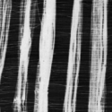
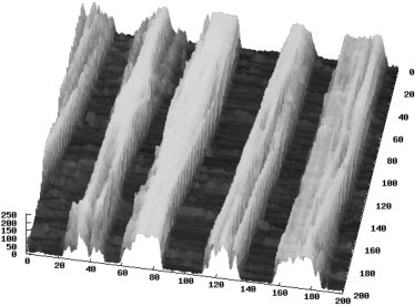
Figure 1: The environment of the artificial crawler. On the top is shown a textured image and below its respective 3D surface.

The $N$ artificial crawlers begin with equal energy $e_{init}$ and are placed at random on the surface (pixels) of the textured image:

$$\begin{array}[]{l}p_{0}^{i}=rand(I)\\ e_{0}^{i}=e_{init}\end{array}$$ (2)

Then the evolution process starts following a set of specific rules. The aim of the artificial crawler is to move to areas of higher altitudes in order to absorb energy and sustain life. This way, the next step $p_{t+1}^{i}=f(p_{t}^{i})$ depends on the gray level of its neighbors according to Equation 3. First, the artificial crawler settles down if the gray level of its 8 neighbors are lower than itself (Figure 2 (a)). Second, the artificial crawler moves to a specific pixel if there exist one of its 8 neighbors with unique higher intensity (Figure 2 (b)). Third, if there exist more than one neighbor with higher intensity, an artificial crawler moves to the pixel that was already occupied by another artificial crawler in any time (Figure 2 (c)). Otherwise, it moves to one of the pixels randomly.

$$f(p_{t}^{i})=\left\{\begin{array}[]{lll}p_{t}^{i},&\textrm{if }I(p_{t}^{i})\geq I(p)\,\forall p\in\eta(p_{t}^{i})\\ p,&\textrm{if }I(p)>I(p_{t}^{i}),I(p)>I(q)\,\forall p,q\in\eta(p_{t}^{i}),\\ &p\neq q\\ p,&\textrm{if }I(p)>I(p_{t}^{i}),I(p)\geq I(q)\,\forall p,q\in\eta(p_{t}^{i}),\\ &p\neq q,p\textrm{ was visited}\end{array}\right.$$ (3)

Figure 2: Example of the three possible steps of artificial crawlers considering its 8 neighbors.

Given the new position of the artificial crawler, the energy absorption from the environment is performed:

$$e_{t+1}^{i}=e_{t}^{i}+\lambda I(p_{t+1}^{i})-1$$ (4)

where $\lambda$ is the rate of absorption over the gray level of the current pixel $I(p_{t+1}^{i})$. All artificial crawlers lose a unit of energy which means that the artificial crawler loses energy at each step if $\lambda*I(p_{t+1}^{i})<1$. For the default value of $\lambda=0.01$, it means that the artificial crawler loses energy if it goes to a pixel whose gray level is less than $100$ and gain energy otherwise. The energy is bounded by limit $e_{max}$, i.e. if $e_{t+1}^{i}>e_{max}$ then $e_{t+1}^{i}=e_{max}$. Also, an artificial crawler keep living in the next generation whether its energy is higher than a certain threshold $e_{min}$.

After the energy absorption, the law of the jungle is performed. In this law, an artificial crawler with higher energy eats up another with lower energy if they are in the same pixel, i.e. $A_{t+1}^{i}$ eats up $A_{t+1}^{j}$ if $p_{t+1}^{i}=p_{t+1}^{j},e_{t+1}^{i}\geq e_{t+1}^{j},i\neq j$. This law is inspired in nature and assumes that the artificial crawlers with higher energy are more likely to reach the peaks of the environment.

The evolution process converges to an equilibrium state when no further artificial crawlers are in movement (they are dead or settled down). In the original method, features are extracted by means of the number of artificial crawlers at each iteration and colonial properties. Each texture image is represented by four curves of evolution: (1) curve of living artificial crawlers, (2) curve of settled artificial crawlers, (3) curve of colony formation at certain radius and (4) scale distribution of colonies. This representation has two major drawbacks: (i) the vector obtained is high-dimensional, which lead us to the curse of dimensionality and (ii) the extraction of this vector is very time-consuming due to the colony estimation.

III Fractal Dimension

In 1977, Mandelbrot introduced a new mathematical concept to model natural phenomena, named fractal geometry mandelbrot1977 . This formulation received a lot of attention due to its ability to describe irregular shapes and complex objects that Euclidean geometry fails to analyze. In contrast, fractal geometry assumes that an object holds a non-integer dimension. Thus, estimating the fractal dimension of an object is basically related to its complexity. The patterns are characterized in terms of space occupation and self-similarity at different scales. The interactive construction process of the Von Koch curve is a typical example of self-similarity of fractals mandelbrot1983 .

The first definition of dimension was proposed by the Hausdorff-Besicovitch measure hausdorffMA1919 , which provided the basis of the fractal dimension theory. He defined a dimension for point sets as a fraction greater than their topological dimension. Formally, given $X\in\Re^{d}$, a geometrical set of points, the Hausdoff-Besicovitch dimension $D_{H}(X)$ is calculated by:

$$D_{H}(X)=inf\{s:H^{s}(X)=0\}=sup\{H^{s}(X)=\infty\}$$ (5)

where $H^{s}(X)$ is the $s$-dimensional Hausdorff measure (in Equation 6).

$$H^{s}(X)=\lim_{\delta\to 0}inf\left[\sum_{i=1}^{\infty}|U_{i}|^{s}:U_{i}\textrm{ is a }\delta\textrm{-cover of }X\right]$$ (6)

where $|.|$ stands for the diameter in $\Re^{d}$, i.e $|U|=sup|x-y|:x,y\in U$.

In image analysis, the use of the Hausdoff-Besicovitch definition may be impracticable theilerJOSA1990 . An alternative definition generalized from the topological dimension is commonly used. According to this definition, the fractal dimension D of an object $X$ is:

$$D(X)=\lim_{\epsilon\to 0}\frac{\log N(\epsilon)}{\log\frac{1}{\epsilon}}$$ (7)

where $N(\epsilon)$ stands for the number of objects of linear size $\epsilon$ needed to cover the whole object $X$.

There are a lot of algorithms to estimate the fractal dimension of objects or surfaces. The most known algorithms are: box-counting russellPRL1980 , differential box-counting chaudhuriPAMI1995 , $\epsilon$-blanket pelegPAMI1984 , fractal model based on Fractional Brownian motion pentlandCSCVPR1983 , power spectrum method pentlandCSCVPR1983 , Bouligand-Minkowski tricot1995 among others; as well as extensions of fractals, such as multifractals chaudhariASS2004 , multi-scale fractals odemirIS2008 and fractal descriptors BackesCB12 ; FlorindoBCB12 ; FlorindoB12 ; FlorindoSPB13 . One of the most accurate methods to estimate the fractal dimension is the Bouligand-Minkowski method tricot1995 ; odemirIS2008 ; backesIJPRAI2009 . The Boulingand-Minkowski fractal dimension $D_{B}(X)$ depends on a symmetrical structuring element $Y$:

$$\begin{array}[]{l}D_{B}(X,Y)=inf\{\lambda,m_{B}(X,Y,\lambda)=0\}\\ \\ m_{B}(X,Y,\lambda)=\lim_{\epsilon\to 0}\frac{V(\partial X\oplus\epsilon Y)}{\epsilon^{n-\lambda}}\end{array}$$ (8)

where $m_{B}$ is the Bouligand-Minkowski measure, $\epsilon$ is the radius of the element $Y$ and $V$ is the volume of the dilation between element $Y$ and boundary $\partial X$. To eliminate the explicit dependence on the element $Y$, a simplified version of the Bouligand-Minkowski fractal dimension can be described by using neighborhood techniques as:

$$D_{B}(X)=\lim_{\epsilon\to 0}\left(D_{T}-\frac{\log V(X\oplus Y_{\epsilon})}{\log\epsilon}\right)$$ (9)

For instance considering an object $X\in\Re^{3}$, the topological dimension $D_{T}=3$ and $Y_{\epsilon}$ is a sphere of diameter $\epsilon$. Varying the radius $\epsilon$, it estimates the fractal dimension based on the size of the influence area $V$ created by the dilation of $X$ by $Y_{\epsilon}$.

IV Proposed Method

In this section, we describe the proposed method, which is based on the fractal dimension of artificial crawlers. Basically, our method can be divided into two parts: artificial crawlers are performed in the texture image and then the fractal dimension of these artificial crawlers is estimated. The next sections describe these steps of our method.

IV.1 Artificial Crawler Model in Images

Although the original artificial crawler method achieves promising results, the idea of moving to pixels with higher intensities does not extract all the richness of textural pattern of the images. In the method proposed here, the independent artificial crawler is also able to move to lower intensities (valleys). It allows the model to take full advantage and capture the richness of details present in peaks and valleys of the images.

In the first step, the artificial crawlers move to higher intensities as the original method. Thus, artificial crawlers $A^{i}_{T}=\{p_{T}^{i},e_{T}^{i}\}$ are obtained after the evolution process converges, where $T$ is the number of step needed to the system converges. Throughout the paper, the artificial crawlers which move to higher intensities will be referred to as $U_{T}^{i}=\{p_{T}^{i},e_{T}^{i}\}$ and this rule of movement will be referred to as $max$. Figure 3 shows an example of 1000 artificial crawlers using the rule of movement $max$. Although the image in Figure 3(a) is an elaborate example we present how the agents find the maxima accordingly the $max$ rule. The green marks stand for the final position (convergence) of the live artificial crawler while the red ones represent the final position of the dead artificial crawlers. As we can see, the live artificial crawlers can achieve the highest intensities. The energy of these artificial crawlers implicitly stores all the information along the steps and this energy is important to represent the surface that the artificial crawler is emerged. As important as the live artificial crawler’s, the dead ones aggregate information from the surface of the environment.

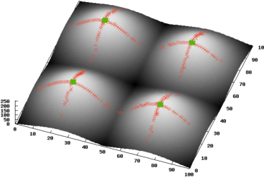
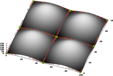
Figure 3: The final position of 1000 artificial crawlers, (a) by using the rule of movement $max$ and (b) by using the rule of movement $min$. Green marks stand for live artificial crawlers while red marks represent dead artificial crawlers.

In Figure 3, we can observe that the original method only describes the peaks of a texture image. In addition, we propose to move artificial crawlers toward lower intensities. In this approach, artificial crawlers $Q_{t}^{i}=\{p_{T}^{i},e_{T}^{i}\}$ are randomly placed in the image with initial energy $e_{init}$. Then, the evolution process is modified so that the next step of an artificial crawler is to move towards the lower intensity (Equation 10). This rule of movement will be referred to throughout the paper as $min$.

$$f(p_{t}^{i})=\left\{\begin{array}[]{lll}p_{t}^{i},&\textrm{if }I(p_{t}^{i})\leq I(p)\,\forall p\in\eta(p_{t}^{i})\\ p,&\textrm{if }I(p)<I(p_{t}^{i}),I(p)<I(q)\,\forall p,q\in\eta(p_{t}^{i}),\\ &p\neq q\\ p,&\textrm{if }I(p)<I(p_{t}^{i}),I(p)\leq I(q)\,\forall p,q\in\eta(p_{t}^{i}),\\ &p\neq q,p\textrm{ was visited}\end{array}\right.$$ (10)

An example of the artificial crawlers using the rule of movement $min$ can be seen in Figure 3 (b). Again, green marks represent the final position of live artificial crawlers while red marks represent the dead artificial crawlers. These artificial crawlers complement the artificial crawlers that use the rule of movement $max$, aggregating more information about the surface.

In the end of this step, we have two populations of $N$ artificial crawlers $U_{T}^{i}=\{p_{T}^{i},e_{T}^{i}\}$ and $Q_{T}^{i}=\{p_{T}^{i},e_{T}^{i}\}$ which correspond to the artificial crawlers using rules of movement $max$ and $min$, respectively.

IV.2 Fractal Dimension of Artificial Crawler

In this section, we describe how to quantify the population of artificial crawlers using the fractal dimension theory. To estimate the fractal dimension using the Boulingand-Minkowski method, the population of artificial crawlers can be easily mapped onto a surface $S\in\Re^{3}$, by converting the position $p_{T}^{i}=\{x_{i},y_{i}\}$ and the energy $e_{T}^{i}$ of each artificial crawler into a 3D point $s_{i}=(x_{i},y_{i},e_{T}^{i})$. The energy is important because it contain all the information of the artificial crawler steps. This mapping can be seen in Figure 4 (a). We should note that the $Z$ axis is the energy of the artificial crawler.

The Boulingand-Minkowski method estimates the fractal dimension based on the size of the influence area $|S(r)|$ created by the dilation of $S$ by a radius $r$. Thus varying the radius $r$, the fractal dimension of surface $S$ is given by:

$$D=3-\lim_{r\to 0}\frac{log\,V(r)}{log\,r}$$ (11)

where $V(r)$ is the influence volume obtained through the dilation process of each point of $S$ using a sphere of radius $r$:

$$V(r)=|\{s^{\prime}\in\Re^{3}\mid\exists s\in S:|s-s^{\prime}|\leq r\}|$$ (12)

The dilation process is illustrated in Figure 4. A group of artificial crawlers are mapped onto a 3D space, shown in Figure 4 (a). Each point of the 3D space is dilated by a sphere of radius $r$ (Figure 4 (b) and (c)). As the value of radius $r$ is increased, more collisions are observed among the dilated spheres. These collisions disturb the total influence volume $V(r)$, which is directly linked to the roughness of the surface.

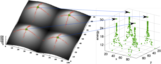
(a) Artificial crawlers mapped onto a 3D space by converting the final position and the energy into a point in the surface.

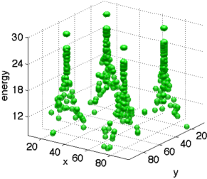
(b) $r=2$

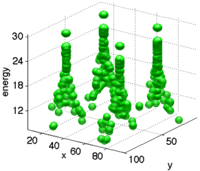
(c) $r=3$

Figure 4: An illustration of the dilation process for the fractal dimension estimation of artificial crawlers. The final position of the artificial crawlers was obtained using the rule of movement $max$ and maximum energy $e_{max}=30$.

From the linear regression of the plot of $\log r\times\log V(r)$, the Boulingand-Minkowski fractal dimension is computed by:

$$D=3-\alpha$$ (13)

where $\alpha$ is the slope of the estimated line.

IV.3 Feature Vector

Although the fractal dimension provides a robust mathematical model, it describes each object by only one real value $D$ $-$ the fractal dimension. Objects with distinct shapes can have the same fractal dimension, for instance, the very well know fractals :Peano curve, Dragon curve, Julia set and the boundary of the Mandelbrot set have the same Hausdorff dimension equals to 2. To overcome this characteristic the concept of multi-scale fractal dimension odemirIS2008 and the fractal descriptors BackesCB12 ; FlorindoBCB12 was developed. In this way, the fractal dimension of the object is considered in different scales. It provides a rich shape descriptor that can be successful to discriminate shape and patterns odemirIS2008 .

In odemirIS2008 it was demonstrate

In order to improve the discrimination power of our method, we use the entire curve $V(r)$ instead of using only the fractal dimension:

$$\varphi_{\tau}=[V(1),\dots,V(r_{m})]$$ (14)

where $\tau$ is the rule of movement used by the artificial crawler and $r_{m}$ is the maximum radius.

Considering that we have two rules of movement, the final feature vector is composed by the concatenation of $\varphi_{max}$ and $\varphi_{min}$ according to Equation 15. The feature vectors $\varphi_{max}$ and $\varphi_{min}$ are obtained by using the fractal dimension estimation of acrawlers $U_{T}^{i}$ and $Q_{T}^{i}$ after the stabilization, respectively.

$$\varphi=[\varphi_{max},\varphi_{min}]$$ (15)

The importance of using both rules is corroborated in Figure 5. Figures 5 (b) and (d) show the feature vectors by using $\varphi_{max}$ only, and Figures 5 (c) and (e) show the feature vectors by using $\varphi_{min}$ only. An example of those feature vectors are obtained for four different image classes, as shown in Figure 5 (a). For clarify, each class contains 10 samples. The classes D16 and D18 are discriminated using the rule of movement $max$ (Figure 5 (b)), while the rule of movement $min$ is not able to discriminate those two classes accordingly (Figure 5 (c)). On the other hand, the classes D49 and D93 are only discriminated if the rule of movement $min$ is used (Figure 5 (e)). These plots corroborate the importance of using both rules of movement for texture recognition.

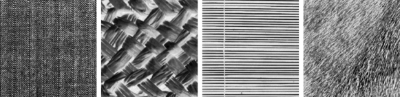
(a) Classes of texture D16, D18, D49 and D93.

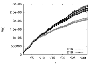
(b) $\varphi_{max}$ for classes D16 and D18.

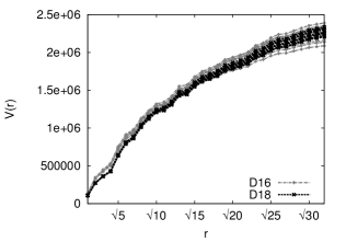
(c) $\varphi_{min}$ for classes D16 and D18.

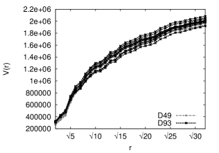
(d) $\varphi_{max}$ for classes D49 and D93.

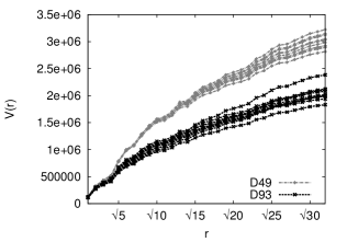
(e) $\varphi_{min}$ for classes D49 and D93.

Figure 5: An example of feature vectors using the rules of movement $min$ and $max$. The classes of texture are only discriminated if both rules are used.

IV.4 Computational Complexity

In the proposed method, $N$ artificial crawlers are performed in the image of size $W\times W$ pixels. The swarm system converges after $M$ steps, which leads to a computational complexity of $O(NM)$. After stabilization, we propose to quantify the swarm system by means of the fractal dimension. To calculate the dilation process, the Euclidean distance transform fabbri2008 is a powerful and efficient tool. This transform calculates the distance between each point of the 3D space and the surface. Several authors saito1994 ; meijster2000 ; fabbri2008 proposed algorithms for computing Euclidean distance transform in linear time. The time complexity is linear in the number of points of the 3D space, which is $O(W\times W\times e_{max})$ $-$ $W\times W$ is the size of the image and $e_{max}$ is the maximum energy of the agents. Usually, the maximum energy $e_{max}$ is a small number (e.g. in this work the maximum energy is $20$). Thus, we can ignore $e_{max}$ in the complexity, since $W\gg 20$ in image applications. Finally the computational complexity of the proposed method is stated as $O(NM+W^{2})$.

Let us discuss the best, worst and average case based on the number of steps of the swarm system. The best case considers that the swarm system converges in one step ($M=1$). Thus, the computation complexity is $O(N+W^{2})$. In the worst case, the swarm system takes more than $N$ steps, however it is stopped in $M=N$ steps without the stabilization. The worst case leads to a complexity of $O(N^{2}+W^{2})$. It is important to emphasize that the worst case rarely occurs, requiring a specific configuration of the texture image and even a random image does not produce this special case. In order to analyze the average case, we plot in Figure 6 the average number of steps needed to converge over 400 images. We can see that the two rules of movement $min$ and $max$ present similar behavior. Also, the number of agents does not influence the number of steps to converge (e.g. the difference of the average number os steps for $N=5k$ and $N=40k$ is only $1.03$ steps). Given that $M\sim 13$ for $N=50k$, the average case leads to a complexity which is very close to the best case, $O(N+W^{2})$, and it is a good complexity in comparison to the complexities of Gabor filters $O(W^{2}\log W)$ and co-occurrence matrices O($W^{2}$).

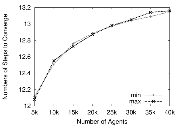
Figure 6: Average number of steps to converge using the rules of movement $min$ and $max$. The average number of steps was averaged over 400 images.

V Experimental Results

In order to evaluate the proposed method, experiments were carried out on image datasets of high variability. We first describe such datasets, the experiments to evaluate the parameters of our proposed method, and then the comparative results with the state-of-the-art methods.

We performed experiments on the two most used image datasets of texture: Brodatz and Vistex. The Brodatz album Brodatz1966 is the most known benchmark for evaluating texture methods. Each class is composed by one image divided into ten non-overlapped samples. The samples have $200\times 200$ pixels with 256 gray levels. In this work, a total of 40 classes with 10 samples per class were used. One example of each class is shown in Figure 7.

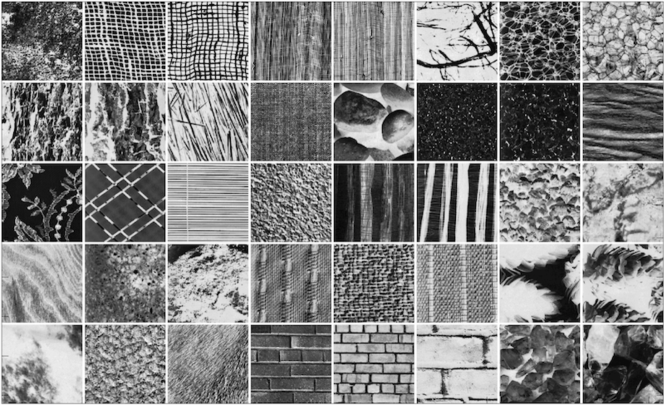
Figure 7: An example of the classes from the Brodatz dataset. Each class has 10 samples of $200\times 200$ pixels and 256 gray levels.

The Vision Texture $-$ Vistex SinghICAPR2001 provides real-world textures under challenging conditions (e.g. lighting and perspective). A total of 54 classes are available, each class containing 16 samples. The samples have $128\times 128$ pixels with 256 gray levels. Figure 8 presents one example of each class.

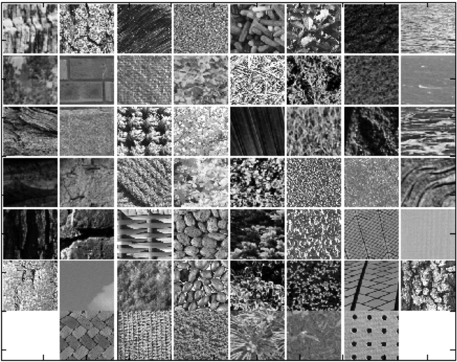
Figure 8: An example of the classes from the Vistex dataset. Each class has 16 samples of $128\times 128$ pixels and 256 gray levels.

In our experiments, Linear Discriminant Analysis (LDA) timm2002applied ; Fukunaga1990 in a 10-fold cross-validation strategy was adopted in the task of classification. The LDA method estimates a linear subspace in which the projection of the vectors presents larger variance inter-classes than the variance intra-classes. The 10-fold cross-validation strategy divides randomly the samples into 10 folds. Each fold is used to test the classifier while the other nine folds are used to train the classifier. This process is repeated 10 times with each fold used once as testing data. To produce a single statistic, the results of the 10 processes are averaged.

The features used in this paper, and the parameter evaluation are in the next section.

V.1 Parameter Evaluation

In this section, we evaluate the three main parameters of our method: number of artificial crawlers $N$, maximum energy $e_{max}$ and maximum radius $r_{m}$ of the fractal dimension. The other parameters were set according to ZhangIJPRAI2005 , since their possible values do not affect the final success rate. Each artificial crawler is born with initial energy $e_{init}=10$, the survival threshold $e_{min}=1$ and the absorption rate $\lambda=0.01$.

The success rates for the different number of artificial crawlers are shown in Figure LABEL:fig:n for both Brodatz and Vistex datasets. The number of artificial crawlers placed on the pixels were initially set to $5k$ with a coverage rate of 5%, varying from $5k$ to $40k$ for the Brodatz dataset and varying from $5k$ to $15k$ for the Vistex dataset due to the size of the samples ($128\times 128$ pixels). We can observe that the highest success rate was obtained for $N=30k$ and $N=15k$ for the Brodatz and Vistex, respectively. Further, it was found that the combination of rules $min$ and $max$ significantly improve the success rate for all number of artificial crawlers in both datasets. Also, the rule of going to the minimum intensity provides similar results to the original rule $-$ $max$. These results suggest that the valleys and peaks are important to obtain a robust texture analysis.

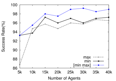
(a) Brodatz

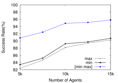
(b) Vistex.

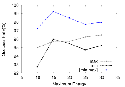
(c) Brodatz

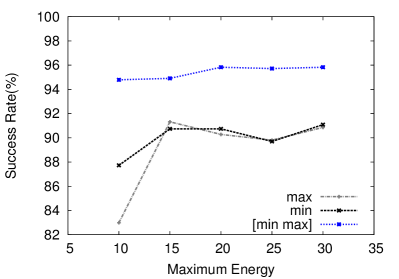
(d) Vistex.

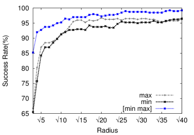
(e) Brodatz

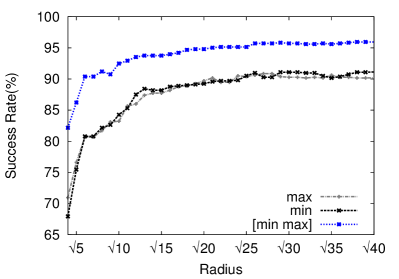
(f) Vistex.

Figure 9: Plots for different The plot for evaluating the number of artificial crawlers in the Brodatz and Vistex datasets.

The maximum energy of the artificial crawlers is evaluated in the plot of the Figure 9. Figure 9 (c) presents the results for the Brodatz dataset while Figure 9 (d) shows the results for the Vistex dataset. The maximum energy parameter was evaluated by the fact that it limits the artificial crawler energy and, consequently, can limit the fractal dimension space. However, the experimental results show that different values of maximum energy do not influence the success rate considerably. The highest success rate was obtained for $e_{max}=15$ using the Brodatz dataset and for $e_{max}=20$ using the Vistex dataset. It can be noted that the same behavior for the rules of movement was obtained here, with the combination of rules providing the highest success rates.

In the plot of Figure 9, the maximum radius of the fractal dimension estimation is evaluated. As expected, the success rate increases as the radius increases and stabilizes after a certain radius. The maximum radius $r_{m}=\sqrt{37}$ provided the highest success rate of $99.25\%$ for the Brodatz dataset. For the Vistex dataset, a success rate of $95.95\%$ was obtained by the maximum radius $r_{m}=\sqrt{38}$. As the previous results, the combination of rules of movement provides the highest success rates. Also, the rule $min$ provides similar results compared to the rule $max$. Using these plots, we can set the parameters of the proposed method for the Brodatz dataset to $N=30k$, $e_{max}=15$, $r_{m}=\sqrt{37}$. For the Vistex dataset, the parameters are $N=15k,e_{max}=20$ and $r_{m}=\sqrt{38}$, which are close to the best parameters for the Brodatz dataset. For other datasets, we recommend using a number of agents $N$ between $60\%$ and $95\%$ of the number of pixels, $10\leq e_{max}\leq 25$ and $\sqrt{30}\leq r_{m}\leq\sqrt{40}$.

V.2 Comparison with other Methods

The proposed method, which is enriched by the fractal dimension estimation of artificial crawler, is compared to traditional texture methods, namely Fourier descriptors azencottPAMI1997 , co-occurrence matrices ChristophPR2004 ; haralickTSMC1973 , Gabor filter Bianconi2007 ; Jain1991 ; gaborJIEE1946 , local binary pattern Ojala2002 , and multi fractal spectrum Xu2009 . Moreover, the texture method using the artificial crawlers proposed in ZhangIJPRAI2005 was also used in this comparison. We considered the traditional implementation of each method and its parameter configuration as described below, which yields the best result.

Fourier descriptors: these descriptors are obtained from the Fourier transform of the texture image. Each descriptor is the sum of the spectrum values within a radius from the center. The best results were obtained by radius with increment by one. Thus, for an image of $200\times 200$ pixels, 99 descriptors are obtained. More information about the Fourier descriptors can be found in azencottPAMI1997 .

Co-occurrence matrices: they are computed by the joint probability distribution between pairs of pixels at a given distance and direction. In these experiments, we consider the distances from 1 to 5 pixels, and the angles $0^{o}$, $45^{o}$, $90^{o}$ and $135^{o}$. Energy and entropy were calculated from these matrices to compose a 40-dimensional feature vector haralickTSMC1973 ; ChristophPR2004 .

Gabor filters: it convolves an image by a bank of Gabor filters (i.e., different scales and orientations). In the experiments, a bank of 40 filters (8 rotations and 5 scales) was used. The energy of each convolved image is used compose the feature vector; in this case a 40-dimensional feature vector. Additional information can be found in Bianconi2007 ; Jain1991 ; gaborJIEE1946 .

Artificial crawlers: $N$ artificial crawler, as those explained earlier, are performed in a texture image. Four features vectors are then calculated: (i) the number of live artificial crawlers at each iteration, (ii) the number of settled artificial crawlers at each iteration, (iii) a histogram of the colony size formed by a certain radius and (iv) scale distribution of the colonies. Finally, the four features vectors are concatenated to compose a single vector. A complete description of the original method can be found in ZhangIAT2004 ; ZhangIJPRAI2005 .

Deterministic tourist walk: this method backesPR2010 is an agent-based method that builds a joint probability distribution of transient and attractor sizes for different values of memory sizes and two walking rules. In the experiments below, we used memory sizes ranging from $0$ to $5$.

Multi Fractal Spectrum: this method Xu2009 extracts the fractal dimension of three categorization of the image: intensity, energy of edges, and energy of the Laplacian. For each categorization, a 26-dimensional MFS vector of uniformly spaced values was computed, totaling a feature vector of 78 dimensions.

Uniform rotation-invariant local binary pattern: the LBP method Ojala2002 calculates the co-occurrence of gray-levels in circular neighborhoods. We used three different spatial resolutions $P$ and three different angular resolutions $R$ $-$ $(P,R)$: (8,1), (16,2) and (24,3).

In Table 1 we present the comparison of the texture methods on the Brodatz dataset. The proposed method provided comparable results to the local binary patterns and superior results to the other state-of-the-art methods. Though local binary patterns features perform slightly better than ours, the test also indicates that the proposed method significantly improves the success rate over the original artificial crawler, i.e., from 89.75% to 99.25%. Despite of the Brodatz dataset is widely used for texture classification, it does not contains textures with changes in terms of lighting conditions and perspectives.

Table 1: The experimental results for texture methods in the Brodatz database.

Method	Correctly classified	Success rate
Fourier descriptors	346	86.50 ($\pm 6.58$)
Artificial Crawler	359	89.75 ($\pm 4.76$)
Co-occurrence matrices	365	91.25 ($\pm 2.65$)
Multi Fractal Spectrum	373	93.25 ($\pm 2.37$)
Gabor filter	381	95.25 ($\pm 3.43$)
Deterministic tourist walk	382	95.50 ($\pm 3.12$)
Local binary patterns	399	99.75 ($\pm 0.79$)
Proposed method	397	99.25 ($\pm 1.69$)

To evaluate the methods in textures closer to real-world applications, we also compared the results for the Vistex dataset which are presented in Table 2. In this test, our method provided the highest success rate of $95.95\%$, which is superior to the result of the local binary patterns. Our method significantly improved the success rate compared to the original artificial crawler. Besides, it can be noted that our method achieved reliable results according to the low standard deviations in both datasets.

Table 2: Experimental results for texture methods in the Vistex database.

Method	Correctly classified	Success rate
Fourier descriptors	672	77.78 ($\pm 4.67$)
Artificial Crawler	691	79.98 ($\pm 4.65$)
Co-occurrence matrices	663	76.74 ($\pm 4.91$)
Deterministic tourist walk	734	84.95 ($\pm 4.13$)
Multi Fractal Spectrum	747	86.46 ($\pm 3.48$)
Gabor filter	774	89.58 ($\pm 2.61$)
Local binary patterns	801	92.71 ($\pm 2.43$)
Proposed method	829	95.95 ($\pm 2.50$)

VI Conclusion

In this paper we have proposed a new method based on artificial crawler and fractal dimension for texture classification. We have demonstrated how the feature vector extraction task can be improved by combining two rules of movement, instead of moving only for the maximum intensity of the neighbor pixels. Moreover, a strategy using fractal dimension was proposed to characterize the path of movement performed by the artificial crawlers. The idea of our approach improves the ability of discrimination obtained from the swarm system of artificial crawlers.

Although traditional methods of texture analysis – e.g. Gabor filters, local binary patterns, and co-occurrence matrices – have provided satisfactory results, the method proposed here has proved to be superior for characterizing textures on the Vistex dataset. On the Brodatz album, our method achieve the second place, being slightly inferior to the local binary pattern method. Experiments on both datasets indicate that our method significantly improved the classification rate with regard to the original artificial crawler method. As future work, we believe that performance gains can be achieved by means of effective descriptors, for example for representing shape.

References

- (1) R. M. Haralick, K. Shanmugam, I. Dinstein, Textural features for image classification, IEEE Transactions on Systems, Man and Cybernetics 3 (6) (1973) 610–621.
- (2) R. M. Haralick, Statistical and structural approaches to texture, Proceedings of the IEEE 67 (5) (1979) 786–804.
- (3) R. L. Kashyap, A. Khotanzad, A model-based method for rotation invariant texture classification, IEEE Trans. Pattern Anal. Mach. Intell. 8 (1986) 472–481.
- (4) D. Chetverikov, Texture analysis using feature based pairwise interaction maps, Pattern Recognition 32 (3) (1999) 487–502.
- (5) G. R. Cross, A. K. Jain, Markov random field texture models, IEEE Trans. Pattern Anal. Mach. Intell. 5 (1983) 25–39.
- (6) R. Chellappa, S. Chatterjee, Classification of textures using gaussian markov random fields, IEEE Transactions on Acoustics, Speech, and Signal Processing 33 (1) (1985) 959–963.
- (7) R. Azencott, J.-P. Wang, L. Younes, Texture classification using windowed fourier filters, IEEE Trans. Pattern Anal. Mach. Intell. 19 (1997) 148–153.
- (8) D. Gabor, Theory of communication, Journal of Institute of Electronic Engineering 93 (1946) 429–457.
- (9) B. B. Machado, W. N. Gonçalves, O. M. Bruno, Enhancing the texture attribute with partial differential equations: a case of study with gabor filters, in: Proceedings of the 13th international conference on Advanced concepts for intelligent vision systems, ACIVS’11, Springer-Verlag, Berlin, Heidelberg, 2011, pp. 337–348.
-
(10)
S. G. Mallat, A theory for
multiresolution signal decomposition: The wavelet representation, IEEE
Trans. Pattern Anal. Mach. Intell. 11 (7) (1989) 674–693.
doi:10.1109/34.192463.
URL http://dx.doi.org/10.1109/34.192463 -
(11)
S. Arivazhagan, L. Ganesan,
Texture classification
using wavelet transform, Pattern Recogn. Lett. 24 (9-10) (2003) 1513–1521.
doi:10.1016/S0167-8655(02)00390-2.
URL http://dx.doi.org/10.1016/S0167-8655(02)00390-2 - (12) J. Serra, Image Analysis and Mathematical Morphology, Academic Press, Inc., Orlando, FL, USA, 1983.
- (13) Y. Chen, E. Dougherty, Gray-scale morphological granulometric texture classification, Optical Engineering 33 (8) (1994) 2713–2722.
- (14) B. B. Mandelbrot, The Fractal Geometry of Nature, W. H. Freeman and Company, New York, 1983.
- (15) O. M. Bruno, R. de Oliveira Plotze, M. Falvo, M. de Castro, Fractal dimension applied to plant identification, Information Sciences 178 (2008) 2722–2733.
- (16) J. Liu, Y. Y. Tang, Adaptive image segmentation with distributed behavior-based agents, IEEE Trans. Pattern Anal. Mach. Intell. 21 (6) (1999) 544–551.
- (17) K.-W. Wong, K.-M. Lam, W.-C. Siu, A novel approach for human face detection from color images under complex background, Pattern Recognition 34 (10) (2001) 1993–2004.
- (18) V. Rodin, A. Benzinou, A. Guillaud, P. Ballet, F. Harrouet, J. Tisseau, J. L. Bihan, An immune oriented multi-agent system for biological image processing, Pattern Recognition 37 (4) (2004) 631–645.
- (19) S.-M. Guo, C.-S. Lee, C.-Y. Hsu, An intelligent image agent based on soft-computing techniques for color image processing, Expert Syst. Appl. 28 (2005) 483–494.
- (20) R. Billon, A. Nédélec, J. Tisseau, Gesture recognition in flow based on pca analysis using multiagent system, in: Proceedings of the International Conference on Advances in Computer Entertainment Technology, ACM International Conference Proceeding Series, ACM, 2008, pp. 139–146.
- (21) A. R. Backes, W. N. Gonçalves, A. S. Martinez, O. M. Bruno, Texture analysis and classification using deterministic tourist walk, Pattern Recogn. 43 (2010) 685–694.
- (22) W. N. Gonçalves, O. M. Bruno, Combining fractal and deterministic walkers for texture analysis and classification, Pattern Recognition 46 (11) (2013) 2953–2968.
- (23) W. N. Gonçalves, O. M. Bruno, Dynamic texture analysis and segmentation using deterministic partially self-avoiding walks, Expert Systems with Applications 40 (11) (2013) 4283–4300.
- (24) H. Zheng, A. Wong, S. Nahavandi, Hybrid ant colony algorithm for texture classification, in: The 2003 Congress on Evolutionary Computation, CEC ’03, Piscataway, N.J., Canberra, Australia, 2003, pp. 2648–2652.
- (25) D. Zhang, Y. Q. Chen, Classifying image texture with artificial crawlers, in: Proceedings of the IEEE/WIC/ACM International Conference on Intelligent Agent Technology, IAT ’04, IEEE Computer Society, Washington, DC, USA, 2004, pp. 446–449.
- (26) D. Zhang, Y. Q. Chen, Artificial life: a new approach to texture classification, International Journal of Pattern Recognition and Artificial Intelligence 19 (3) (2005) 355–374.
- (27) C. Tricot, Curves and fractal dimension, Springer-Verlag, 1995.
- (28) B. B. Mandelbrot, Fractals: form, chance, and dimension, Mathematics Series, W. H. Freeman, San Francisco (CA, USA), 1977.
- (29) F. Hausdorff, Dimension und äusseres mass, Mathematische Annalen 79 (1919) 157–179.
- (30) J. Theiler, Estimating fractal dimension, J. Opt. Soc. Am. A 7 (6) (1990) 1055–1073.
- (31) D. A. Russell, J. D. Hanson, E. Ott, Dimension of strange attractors, Physical Review Letters 45 (14) (1980) 1175–1178.
- (32) B. B. Chaudhuri, N. Sarkar, Texture segmentation using fractal dimension, IEEE Trans. Pattern Anal. Mach. Intell. 17 (1995) 72–77.
- (33) S. Peleg, J. Naor, R. Hartley, D. Avnir, Multiple resolution texture analysis and classification, IEEE Transactions on Pattern Analysis and Machine Intelligence 6 (4) (1984) 518–523.
- (34) A. Pentland, Fractal-based description of natural scenes, in: Proc. of the IEEE Computer Society Conf. on Computer Vision and Pattern Recognition, 1983, pp. 201–209.
- (35) A. Chaudhari, C.-C. S. Yan, S.-L. Lee, Multifractal analysis of growing surfaces, Applied Surface Science 238 (1-4) (2004) 513–517.
- (36) D. C. André R. Backes, O. M. Bruno, Color texture analysis based on fractal descriptors, Pattern Recognition 45 (5) (2012) 1984–1992. doi:10.1016/j.patcog.2011.11.009.
- (37) M. d. C. João B. Florindo, André R. Backes, O. M. Bruno, A comparative study on multiscale fractal dimension descriptors, Pattern Recognition Letters 33 (6) (2012) 798–806. doi:10.1016/j.patrec.2011.12.016.
- (38) J. ao B. Florindo, O. M. Bruno, Fractal descriptors based on fourier spectrum applied to texture analysis, Physica A 391 (20) (2012) 4909–4922. doi:10.1016/j.physa.2012.03.039.
- (39) J. ao B. Forindo, E. C. P. Mariana S. Sikora, O. M. Bruno, Characterization of nanostructured material images using fractal descriptors, Physica A: Statistical Mechanics and its Applications 392 (7) (2013) 1694–1701. doi:10.1016/j.physa.2012.11.020.
- (40) A. R. Backes, D. Casanova, O. M. Bruno, Plant leaf identification based on volumetric fractal dimension, IJPRAI 23 (6) (2009) 1145–1160.
- (41) R. Fabbri, L. da F. Costa, J. C. Torelli, O. M. Bruno, 2d euclidean distance transform algorithms: A comparative survey, ACM Computing Surveys 40 (1) (2008) 1–44.
- (42) T. Saito, J.-I. Toriwaki, New algorithms for euclidean distance transformation of an n-dimensional digitized picture with applications, Pattern Recognition 27 (11) (1994) 1551–1565. doi:10.1016/0031-3203(94)90133-3.
- (43) A. Meijster, J. B. T. M. Roerdink, W. H. Hesselink, A general algorithm for computing distance transforms in linear time, in: Mathematical Morphology and its Applications to Image and Signal Processing, 2000, pp. 331–340. doi:10.1007/0-306-47025-X\_36.
- (44) P. Brodatz, Textures: A Photographic Album for Artists and Designers, Dover Publications, New York, 1966.
- (45) S. Singh, M. Sharma, Texture analysis experiments with meastex and vistex benchmarks, in: Proceedings of the Second International Conference on Advances in Pattern Recognition, ICAPR ’01, Springer-Verlag, London, UK, 2001, pp. 417–424.
- (46) N. H. Timm, Applied multivariate analysis, Springer texts in statistics, Springer, 2002.
- (47) K. Fukunaga, Introduction to statistical pattern recognition (2nd ed.), Academic Press Professional, Inc., San Diego, CA, USA, 1990.
- (48) C. Palm, Color texture classification by integrative co-occurrence matrices, Pattern Recognition 37 (5) (2004) 965–976.
- (49) F. Bianconi, A. Fernández, Evaluation of the effects of gabor filter parameters on texture classification, Pattern Recognition 40 (12) (2007) 3325 – 3335.
- (50) A. K. Jain, F. Farrokhnia, Unsupervised texture segmentation using gabor filters, Pattern Recognition 24 (12) (1991) 1167–1186.
-
(51)
T. Ojala, M. Pietikäinen, T. Mäenpää,
Multiresolution
gray-scale and rotation invariant texture classification with local binary
patterns, IEEE Trans. Pattern Anal. Mach. Intell. 24 (7) (2002) 971–987.
doi:10.1109/TPAMI.2002.1017623.
URL http://dx.doi.org/10.1109/TPAMI.2002.1017623 -
(52)
Y. Xu, H. Ji, C. Fermüller,
Viewpoint invariant
texture description using fractal analysis, Int. J. Comput. Vision 83 (1)
(2009) 85–100.
doi:10.1007/s11263-009-0220-6.
URL http://dx.doi.org/10.1007/s11263-009-0220-6