A Solution of the Hubbard Model

Abstract

We report a ground-state solution for the two-dimensional fermionic Hubbard model, which is obtained via a numerical variational method. The two ingredients in this approach are tensor network states and the time-evolving block decimation. We easily handle the horizontal hopping in the Hamiltonian, and we proceed further to observe the fermion-exchange effect caused by the vertical hopping. By requiring no divergence and no convergence to zero for the ground state, we successively determine the ground-state energy per site as a function of the chemical potential and the lattice length. In addition, we observe saturation in the behavior of the ground-state energy as the lattice length increases.

1 Introduction

In 1963, to understand the behavior of correlated electrons in solids, a fermion lattice model was proposed independently by three physicists: Martin Gutzwiller [1], Junjiro Kanamori [2], and John Hubbard [3]. This model has become widely known as the Hubbard model [4]. Since this model’s relevance to high $T_{c}$ superconductors was first suggested [5], much attention has been paid to it. Recently, it has become possible to construct experimental implementations of the Hubbard model using an optical lattice for cold atoms [6, 7], and hence, the research community has refocused on the Hubbard model. Although the model can be represented in a simple form, we encounter notorious difficulties [8] when we attempt to find a solution even numerically.

One of the main advances in the field of strongly correlated systems is the establishment of the concept of the renormalization group (RG) [9]. In fact, Wilson also invented the numerical RG (NRG) [10] to solve the Kondo problem [11]. Inspired by the NRG, White proposed the density-matrix RG (DMRG) [12], which has proven to be a great success in the simulation of strongly correlated one-dimensional quantum lattice systems. It has been found that the internal structure of the DMRG can be understood with respect to the matrix-product states (MPS) [13, 14, 15, 16]. For two-dimensional systems, the projected entangled-pair states (PEPS) [17, 18] are introduced. More generally, we call all of these states tensor network states (TNS), and they include MPS, PEPS, tree tensor network states [19], the multiscale entanglement renormalization ansatz [20], and matrix-product projected states [21]. Beyond the spin-block concept, the tensor network method based on the coarse-grained tensor RG [22] has been applied to a classical spin system. The method was refined to the second RG [23, 24] by globally optimizing the truncation scheme and improving the accuracy.

When a total Hamiltonian is written as a sum of local Hamiltonians, Vidal [25, 26] introduced a powerful method called time-evolving block decimation (TEBD) for finding correlation functions. If the total Hamiltonian also has a type of symmetry such as translational invariance, we can use the so-called infinite TEBD [27], in which we assume that the matrices in the TNS have the same form, and we update a few matrices to achieve the ground state. However, because the TNS for the Hubbard model is not an eigenstate of the number operator, the TNS breaks the basic symmetry of particle-number preserving. Furthermore, we do not insist on preserving the translational invariance in the TNS. In consequence, we do not use the infinite TEBD here. We alternatively adopt TEBD and extend it to the case of the Hubbard model using PEPS. If the fermion-exchange effect is involved during the TEBD procedure, a long-range entanglement appears between the tensors of the PEPS. The essence of the Hubbard model is to solve the problem caused by the fermion-exchange effect.

In this paper, we focus on updating the large entangled part in the TNS when we apply TEBD to the Hubbard model. To that end, we first describe the nature of the TNS as an approximate ground state for the Hubbard model. The connections between the tensors in the TNS are represented by three types of bonds: horizontal, vertical, and spin bonds. The set of the TNS is a small subspace of the corresponding huge Hilbert space for the Hubbard model. During the imaginary time evolution in TEBD, we restrict the accessible states to the set of the TNS. Furthermore, in the process of updating bonds, we adjust the proportional factor in front of the state. By requiring no divergence and no convergence to zero for the factor, we determine the form of the TNS for the ground state and the corresponding energy.

This paper is organized as follows. In Sec. 2, a detailed description of the Suzuki-Trotter decomposition is given, and we introduce the tensor network state for the Hubbard model. In Sec. 3, using the Suzuki-Trotter decomposition, we present the framework of the algorithm in the spirit of TEBD. Moreover, in this section, we describe how to update the horizontal, vertical, and spin bonds, and present the method of determining the ground-state energy per site. In Sec. 4, we present consistency checks for the method, and we summarize the numerical results obtained when performing TEBD with small bond dimensions; the bond dimensions should be increased in future works. The results for the ground-state energy show evidence of saturation as the lattice length increases, which indicates that the thermodynamic limit is achieved. We observe the spin-flip symmetry breaking, and present the critical strength of the on-site Coulomb repulsion. In conclusion, we discuss a parallelism for implementation in future work to improve the speed of computing.

2 Hamiltonian and Tensor Network States

We begin by presenting the Hamiltonian for the Hubbard model, which is written as

$$H = -t\sum_{\langle ij\rangle}(c^{\dagger}_{i\uparrow}c_{j\uparrow}+c^{\dagger}_{j\uparrow}c_{i\uparrow}+c^{\dagger}_{i\downarrow}c_{j\downarrow}+c^{\dagger}_{j\downarrow}c_{i\downarrow})$$ (1)

$$+U\sum_{i}(n_{i\uparrow}-\frac{1}{2})(n_{i\downarrow}-\frac{1}{2})-\mu\sum_{i}(n_{i\uparrow}+n_{i\downarrow})$$

$$= H^{\uparrow}_{he}+H^{\uparrow}_{ho}+H^{\uparrow}_{ve}+H^{\uparrow}_{vo}+H^{\downarrow}_{he}+H^{\downarrow}_{ho}+H^{\downarrow}_{ve}+H^{\downarrow}_{vo}+H_{d},$$

where $\langle ij\rangle$ represents nearest-neighbor hopping in a two-dimensional lattice, and $n_{i\uparrow}$ and $n_{i\downarrow}$ are the spin-up and the spin-down number operators, respectively. We let the hopping strength $t$ be 1 and vary the strengths of both the on-site Coulomb repulsion $U$ and the chemical potential $\mu$; the number of fermions is controlled by $\mu$. We divide the hopping term into four parts for each spin, which are denoted by $h$(horizontal), $v$(vertical), $e$(even), and $o$(odd), as shown in Fig. 1. The diagonal Hamiltonian $H_{d}$ for a typical basis contains the last two terms of the on-site repulsion and the chemical potential. The Hubbard model may be the simplest quantum system of interacting fermions on a lattice.

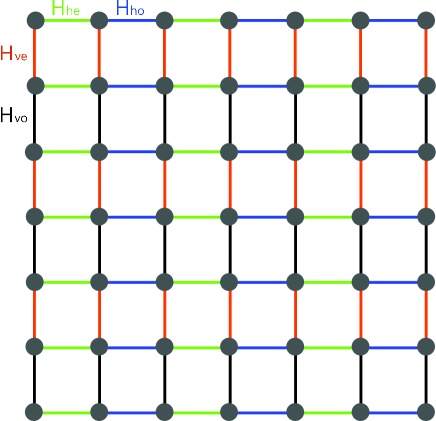
Figure 1: (Color online) Connections between nearby points on the square lattice. The connections are classified into four classes: horizontal-even (denoted by $\langle ij\rangle_{he}$), horizontal-odd, vertical-even, and vertical-odd. Here, the four colors are used to represent four classes, and one hopping Hamiltonian corresponds to each class.

We note that the Hamiltonian has symmetries. First of all, the number operator $N_{op}=\sum_{i}(c^{\dagger}_{i\uparrow}c_{i\uparrow}+c^{\dagger}_{i\downarrow}c_{i\downarrow})$ commutes with the Hamiltonian. When we impose the periodic boundary condition, the translational symmetry appears. Furthermore, the Hamiltonian is invariant under the spin-flip operation such as $c_{i\uparrow}\rightarrow c_{i\downarrow}$ and $c_{i\downarrow}\rightarrow c_{i\uparrow}$. We will discuss these symmetries in relation to the TNS later.

For a given Hamiltonian $H$, we introduce an energy shift $E$ and the inverse of the energy $T$, and then, we consider a formal solution to the imaginary time Schrödinger equation:

$$|\Psi(T)\rangle=\exp\{-(H-E)T\}|\Psi(0)\rangle.$$ (2)

As $T$ goes to infinity, the state $|\Psi(T)\rangle$ becomes the ground state for properly chosen $E$. In fact, when $E$ is larger or smaller than the ground-state energy, $|\Psi(T)\rangle$ blows up or shrinks down, respectively, in the limit as $T\rightarrow\infty$. In a numerical approach, we redefine $E$ as a function of $T$ to determine the ground state.

We rewrite the operator using the Suzuki-Trotter decomposition with a given small time step $\tau$ as

$$\exp\{-(H-E)T\} \cong \prod^{T/\tau}\exp\{(E-H_{d})\tau\}$$ (3)

$$\times \Big{[}\mbox{The same expression for spin down}\Big{]}$$

$$\times \exp(-\frac{1}{4}H^{\uparrow}_{he}\tau)\exp(-\frac{1}{2}H^{\uparrow}_{ho}\tau)\exp(-\frac{1}{4}H^{\uparrow}_{he}\tau)$$

$$\times \exp(-\frac{1}{2}H^{\uparrow}_{ve}\tau)\exp(-H^{\uparrow}_{vo}\tau)\exp(-\frac{1}{2}H^{\uparrow}_{ve}\tau)$$

$$\times \exp(-\frac{1}{4}H^{\uparrow}_{he}\tau)\exp(-\frac{1}{2}H^{\uparrow}_{ho}\tau)\exp(-\frac{1}{4}H^{\uparrow}_{he}\tau).$$

It is not difficult to employ a higher-order Suzuki-Trotter decomposition to obtain a more accurate calculation. Note that we now decompose the operators in Eq. (3) in terms of elementary operators such as

$$\exp(-\frac{1}{4}H^{\uparrow}_{he}\tau)=\prod_{\langle ij\rangle_{he}}\exp\{\frac{1}{4}t\tau(c^{\dagger}_{i\uparrow}c_{j\uparrow}+c^{\dagger}_{j\uparrow}c_{i\uparrow})\},$$

$$~{}~{}~{}~{}~{}~{}~{}~{}\vdots$$

$$\exp\{(E-H_{d})\tau\}=\prod_{i}\exp\{e\tau-U\tau(n_{i\uparrow}-\frac{1}{2})(n_{i\downarrow}-\frac{1}{2})+\mu\tau(n_{i\uparrow}+n_{i\downarrow})\},$$

where $e$ is the energy per site, that is, $E/N$, and $N=\sum_{i}1$. Our strategy is to use Vidal’s TEBD with these elementary operators in a small subset of the Hilbert space. This small subset is composed of the TNS characterized by the fixed bond dimension.

For the fermionic Hubbard model, the usual tensor network states should be suitably modified to describe fermions. In previous works, many such attempts have been made; the Jordan-Wigner strings was noticed in relation to fermions [28], and we find the fermionic projected entangled-pair states [29, 30, 31, 32, 33] and the fermionic multiscale entanglement renormalization ansatz [34, 35, 36, 37] for the ground states. These fermionic modifications share some similarities, but they do not agree with each other completely; thus, they require further investigation. As a first step, we adopt the scheme of Corboz’s fermionic PEPS for our TNS, however for which we do not insist on preserving the fermionic parity.

We use the one-to-one correspondence between a state of the two-state chain and a state of the Fock space. The state of the chain is represented by $\sigma_{i}$ and $\sigma_{N+i}$ for the spin-up and the spin-down, respectively, and the state of the Fock space is written in terms of the creation operators $c^{\dagger}_{i\uparrow}$ and $c^{\dagger}_{i\downarrow}$ as follows:

$$|\sigma_{0}\cdots\sigma_{N-1}\sigma_{N}\cdots\sigma_{2N-1}\rangle$$

$$~{}~{}~{}~{}~{}~{}~{}~{}~{}~{}=(c^{\dagger}_{0\uparrow})^{\sigma_{0}}\cdots(c^{\dagger}_{N-1\uparrow})^{\sigma_{N-1}}(c^{\dagger}_{0\downarrow})^{\sigma_{N}}\cdots(c^{\dagger}_{N-1\downarrow})^{\sigma_{2N-1}}|0\rangle,$$ (4)

where $\sigma_{N+i}=0$ or $1$ means there is a spin-down fermion vacancy or occupancy at the $i$-th site, respectively. It is important to maintain the ordering of the fermions in the state of the Fock space to handle the negative sign caused by the fermion exchange. We adopt the zigzag ordering, which is the approach of numbering sites from left to right and from right to left one by one alternately in horizontal lines. For the example of $N=4\times 4$, the corresponding ordering of sites is

$$\begin{array}[]{ccccccccc}0&1&2&3&{}{}{}{}{}{}\hfil&16&17&18&19\\ 7&6&5&4&{}{}{}{}{}{}\hfil&23&22&21&20\\ 8&9&10&11&{}{}{}{}{}{}\hfil&24&25&26&27\\ 15&14&13&12&{}{}{}{}{}{}\hfil&31&30&29&28\end{array}$$

where the numbers from $0$ to $15$ denote the spin-up sites and the numbers from $16$ to $31$ denote the spin-down sites.

When representing the TNS for the Hubbard model, we should appreciate the area law for the entanglement entropy [38]. Taking into account the square lattice, we include two horizontal bonds and two vertical bonds for each tensor. Because the TNS do not preserve the fermion numbers, it is natural to break the translational symmetry also. Thus, we use different tensors at all sites. In order to consider the general case of the spin-flip symmetry breaking, we introduce different tensors for the spin-down fermions from those for the spin-up fermions. Because the Hubbard model has an on-site interaction, we connect the two tensors of spin-up and spin-down at the same site using the spin bond. In consequence, for each tensor we attach four legs for the right, up, left, and down bonds and one leg for the spin bond as well as the physical index. We assign a Schmidt coefficient vector to each bond. Therefore, for the square system of the length $L$, there are $2L^{2}$ tensors and $2L^{2}\times 2+L^{2}$ Schmidt coefficient vectors in our TNS as shown in Fig. 2. These tensors and vectors will be updated in the process of TEBD with periodic boundary conditions.

A typical one of the $2L^{2}$ tensors, $A_{ruld}^{\sigma s}$, has six indices, among which the physical index $\sigma$ takes a value of $0$ or $1$. For the space-bond degree of freedom, the indices $r$ (right), $u$ (up), $l$ (left), and $d$ (down) run from $0$ to $\chi-1$, where $\chi$ is the bond dimension. For the spin-bond degree of freedom, the index $s$ runs from $0$ to $\kappa-1$, where $\kappa$ is the spin-bond dimension. A state in the space of the tensor network states is written as

$$|\mbox{TNS}\rangle=\sum_{\cdots\sigma\rho\cdots\nu\eta\cdots\alpha\beta\cdots\delta\gamma\cdots} \mbox{Tr}\left[\begin{array}[]{cccc}\ddots&\vdots&\vdots&\\ \cdots&A^{\sigma}_{\uparrow}&B^{\rho}_{\uparrow}&\cdots\\ \cdots&C^{\eta}_{\uparrow}&D^{\nu}_{\uparrow}&\cdots\\ &\vdots&\vdots&\ddots\\ \end{array}\right]\left[\begin{array}[]{cccc}\ddots&\vdots&\vdots&\\ \cdots&A^{\alpha}_{\downarrow}&B^{\beta}_{\downarrow}&\cdots\\ \cdots&C^{\gamma}_{\downarrow}&D^{\delta}_{\downarrow}&\cdots\\ &\vdots&\vdots&\ddots\\ \end{array}\right]$$ (14)

$$\times|\cdots\sigma\rho\cdots\nu\eta\cdots\cdots\alpha\beta\cdots\delta\gamma\cdots\rangle,$$

where we ignore the representation of the internal bond indices on the tensors and all internal bonds are connected by Tr, as shown in Fig. 2. Note that the zigzag ordering puts the physical index $\nu$ before $\eta$ in the spin-like chain basis. The thermodynamic limit will be achieved for $L\rightarrow\infty$ and $\chi,\kappa\rightarrow\infty$.

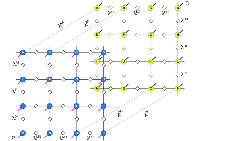
Figure 2: A diagrammatic representation of a coefficient in front of an orthonormal basis of $|\sigma_{0}\cdots\sigma_{N-1}\sigma_{N}\cdots\sigma_{2N-1}\rangle$ for the case of $N=L^{2}=4^{2}$. The closed circles represent $4^{2}\times 2$ six-index tensors. The open diamonds represent the Schmidt coefficients $\lambda$ assigned to each bond. We neglect to draw any spin bonds except the four lines between the spin-up and the spin-down layers. Nevertheless, it should be understood that there are spin bonds between all spin-up and spin-down tensors.

When we consider the case of preserving the spin-flip symmetry, we duplicate the tensors for spin-down using those for spin-up such as

$$|\mbox{TNS}\rangle=\sum_{\cdots\sigma\rho\cdots\nu\eta\cdots\alpha\beta\cdots\delta\gamma\cdots} \mbox{Tr}\left[\begin{array}[]{cccc}\ddots&\vdots&\vdots&\\ \cdots&A^{\sigma}&B^{\rho}&\cdots\\ \cdots&C^{\eta}&D^{\nu}&\cdots\\ &\vdots&\vdots&\ddots\\ \end{array}\right]\left[\begin{array}[]{cccc}\ddots&\vdots&\vdots&\\ \cdots&A^{\alpha}&B^{\beta}&\cdots\\ \cdots&C^{\gamma}&D^{\delta}&\cdots\\ &\vdots&\vdots&\ddots\\ \end{array}\right]$$ (24)

$$\times|\cdots\sigma\rho\cdots\nu\eta\cdots\cdots\alpha\beta\cdots\delta\gamma\cdots\rangle.$$

In the process of TEBD, we update $L^{2}$ tensors and $L^{2}\times(2+1)$ Schmidt coefficient vectors for the ground state preserving the spin-flip symmetry.

The operator $\exp\{(E-H)\tau\}$ of Eq. (3) acts on the state $|\mbox{TNS}\rangle$ of Eq. (5) consecutively. Thus, the output state $\exp\{(E-H)\tau\}|\mbox{TNS}\rangle$, which is outside the space of the TNS, is approximated into a TNS by updating the tensors and the vectors. The updating procedure is the subject of the next section.

3 The Updating Procedure

In order to proceed with TEBD, we consider the single elementary hopping term $\exp\{t\tau(c^{\dagger}_{i\uparrow}c_{j\uparrow}+c^{\dagger}_{j\uparrow}c_{i\uparrow})\}$, where we add a factor of $1/2$ or $1/4$ in front of $t\tau$ if necessary. When the elementary operator acts on the previous TNS, we approximate the output state into our subset of the TNS by updating the tensors and the vectors locally. This procedure is the basic strategy of TEBD.

When the elementary operator $\exp\{t\tau(c^{\dagger}_{i\uparrow}c_{j\uparrow}+c^{\dagger}_{j\uparrow}c_{i\uparrow})\}$ acts on a basis vector $|\sigma_{0}\cdots\sigma_{i}\cdots\sigma_{j}\cdots\sigma_{N-1}\sigma_{N}\cdots\sigma_{2N-1}\rangle$, we find the following important result [39], which is written for four cases that correspond to $\sigma_{i}=0$ or $1$ and $\sigma_{j}=0$ or $1$:

$$\left\{\begin{array}[]{l}\exp\{t\tau(c^{\dagger}_{i\uparrow}c_{j\uparrow}+c^{\dagger}_{j\uparrow}c_{i\uparrow})\}|\cdots 0\cdots 0\cdots\rangle=|\cdots 0\cdots 0\cdots\rangle\\ \exp\{t\tau(c^{\dagger}_{i\uparrow}c_{j\uparrow}+c^{\dagger}_{j\uparrow}c_{i\uparrow})\}|\cdots 0\cdots 1\cdots\rangle=\cosh(t\tau)|\cdots 0\cdots 1\cdots\rangle\\ ~{}~{}~{}~{}~{}~{}~{}~{}~{}~{}~{}~{}~{}~{}~{}~{}~{}~{}~{}~{}~{}~{}~{}~{}~{}~{}~{}~{}+\sinh(t\tau)(-1)^{\sigma_{i+1}+\cdots+\sigma_{j-1}}|\cdots 1\cdots 0\cdots\rangle\\ \exp\{t\tau(c^{\dagger}_{i\uparrow}c_{j\uparrow}+c^{\dagger}_{j\uparrow}c_{i\uparrow})\}|\cdots 1\cdots 0\cdots\rangle=\cosh(t\tau)|\cdots 1\cdots 0\cdots\rangle\\ ~{}~{}~{}~{}~{}~{}~{}~{}~{}~{}~{}~{}~{}~{}~{}~{}~{}~{}~{}~{}~{}~{}~{}~{}~{}~{}~{}~{}+\sinh(t\tau)(-1)^{\sigma_{i+1}+\cdots+\sigma_{j-1}}|\cdots 0\cdots 1\cdots\rangle\\ \exp\{t\tau(c^{\dagger}_{i\uparrow}c_{j\uparrow}+c^{\dagger}_{j\uparrow}c_{i\uparrow})\}|\cdots 1\cdots 1\cdots\rangle=|\cdots 1\cdots 1\cdots\rangle\end{array}\right.$$

The sign of $(-1)^{\sigma_{i+1}+\cdots+\sigma_{j-1}}$ reflects the fermion-exchange effect. Note that the values of the physical indices at the sites numbered from $i+1$ to $j-1$ are related to the sign, which makes it difficult to handle the vertical hopping. The above equations play a key role in updating the TNS.

3.1 Updates to the Horizontal Bonds

Because a horizontal bond connects a site to the next site, that is, to $j=i+1$ in our ordering of sites, it is straightforward to update horizontal bonds. As we can see in the Suzuki-Trotter decomposition of Eq. (3), we first handle $H_{he}$, then $H_{ho}$, and then $H_{he}$ again. Here, we present the typical procedure for updating a horizontal bond.

For example, to update $A$, $B$, and $\lambda^{AB}$ in Fig. 2 with the periodic boundary condition, we consider the tensor product that is represented symbolically as follows:

$$(A\otimes B)^{\sigma s\rho\tilde{s}}_{uld\tilde{r}\tilde{u}\tilde{d}}\equiv\sum_{x=0}^{\chi-1}A^{\sigma s}_{xuld}\lambda^{AB}_{x}B^{\rho\tilde{s}}_{\tilde{r}\tilde{u}x\tilde{d}}\lambda^{AA}_{s}\lambda^{MA}_{u}\lambda^{DA}_{l}\lambda^{AE}_{d}\lambda^{BB}_{\tilde{s}}\lambda^{BC}_{\tilde{r}}\lambda^{NB}_{\tilde{u}}\lambda^{BF}_{\tilde{d}},$$ (25)

where the eight Schmidt coefficients are attached to $A$ and $B$. Using the result of Eq. (7), we find the ten-index tensor $\Theta^{\sigma s\rho\tilde{s}}_{uld\tilde{r}\tilde{u}\tilde{d}}$ to update $A$, $B$, and $\lambda^{AB}$:

$$\left\{\begin{array}[]{l}\Theta^{0s0\tilde{s}}_{uld\tilde{r}\tilde{u}\tilde{d}}=(A\otimes B)^{0s0\tilde{s}}_{uld\tilde{r}\tilde{u}\tilde{d}}\\ \Theta^{0s1\tilde{s}}_{uld\tilde{r}\tilde{u}\tilde{d}}=\cosh(t\tau)\times(A\otimes B)^{0s1\tilde{s}}_{uld\tilde{r}\tilde{u}\tilde{d}}+\sinh(t\tau)\times(A\otimes B)^{1s0\tilde{s}}_{uld\tilde{r}\tilde{u}\tilde{d}}\\ \Theta^{1s0\tilde{s}}_{uld\tilde{r}\tilde{u}\tilde{d}}=\cosh(t\tau)\times(A\otimes B)^{1s0\tilde{s}}_{uld\tilde{r}\tilde{u}\tilde{d}}+\sinh(t\tau)\times(A\otimes B)^{0s1\tilde{s}}_{uld\tilde{r}\tilde{u}\tilde{d}}\\ \Theta^{1s1\tilde{s}}_{uld\tilde{r}\tilde{u}\tilde{d}}=(A\otimes B)^{1s1\tilde{s}}_{uld\tilde{r}\tilde{u}\tilde{d}}\end{array}\right.$$

We emphasize the physical-index exchange between $0$ and $1$ in the tensor product multiplied by $\sinh(t\tau)$. By employing singular value decompositions (SVD), we obtain the updated $\tilde{\lambda}^{AB}_{x}$ by keeping the $\chi$ largest weights:

$$\Theta^{\sigma s\rho\tilde{s}}_{uld\tilde{r}\tilde{u}\tilde{d}} \rightarrow \sum_{x=0}^{\chi-1}\bar{A}^{\sigma s}_{xuld}\tilde{\lambda}^{AB}_{x}\bar{B}^{\rho\tilde{s}}_{\tilde{r}\tilde{u}x\tilde{d}}$$ (26)

$$= \sum_{x=0}^{\chi-1}\tilde{A}^{\sigma s}_{xuld}\tilde{\lambda}^{AB}_{x}\tilde{B}^{\rho\tilde{s}}_{\tilde{r}\tilde{u}x\tilde{d}}\lambda^{AA}_{s}\lambda^{MA}_{u}\lambda^{DA}_{l}\lambda^{AE}_{d}\lambda^{BB}_{\tilde{s}}\lambda^{BC}_{\tilde{r}}\lambda^{NB}_{\tilde{u}}\lambda^{BF}_{\tilde{d}}.$$

By dividing and attaching the eight weights, we find $\tilde{A}$ and $\tilde{B}$ in the above. We denote this process graphically as follows:

$$\begin{array}[]{ccccccccccc}&|&&|&&&&|&&|&\\ -&&\Theta&&-&\rightarrow&-&\tilde{A}&-&\tilde{B}&-\\ &|&&|&&&&|&&|&\end{array}$$

where we omit both the spin bonds and the physical indices.

A similar procedure is performed for other tensors and other vectors. By updating all $2L^{2}$ tensors, we finish the horizontal-bond update. We note that it is possible to update all $2L^{2}$ tensors simultaneously if we use multi-core computers. Thus, we can easily parallelize the horizontal-bond update.

3.2 Updates to the Vertical Bonds

The vertical bonds exhibit a striking difference from the horizontal bonds during the update process: the notorious fermion-exchange effect appears when fermions are hopping vertically. For the vertical bonds, we should consider $\exp\{t\tau(c^{\dagger}_{i\uparrow}c_{j\uparrow}+c^{\dagger}_{j\uparrow}c_{i\uparrow})\}|\cdots\sigma_{i}\cdots\sigma_{j}\cdots\rangle$, where the number of sites between $i$ and $j$ is given by a value from $0$ to $2L-2$ in the zigzag ordering. Therefore, all tensors at the sites between $i$ and $j$ should be updated. Here, we introduce the method for updating the tensors between $i$ and $j$ one by one.

For example, to update $A$, $E$, and $\lambda^{AE}$ on the vertical bond in Fig. 2 with the periodic boundary condition, we begin by writing the tensor product of $A$ and $E$ as follows:

$$\left(\begin{array}[]{l}A\\ \otimes\\ E\end{array}\right){}^{\sigma s\eta\tilde{s}}_{rul\tilde{r}\tilde{l}\tilde{d}}\equiv\sum_{x=0}^{\chi-1}A^{\sigma s}_{rulx}\lambda^{AE}_{x}E^{\eta\tilde{s}}_{\tilde{r}x\tilde{l}\tilde{d}}\lambda^{AA}_{s}\lambda^{AB}_{r}\lambda^{MA}_{u}\lambda^{DA}_{l}\lambda^{EE}_{\tilde{s}}\lambda^{EF}_{\tilde{r}}\lambda^{HE}_{\tilde{l}}\lambda^{EI}_{\tilde{d}}.$$ (27)

From the result of Eq. (7), when the vertical-hopping term acts on the TNS we find the portion that should be updated into a single tensor network:

$$\begin{array}[]{cccccccccccc}&&|&&|&&|&&|&\\ &-&&-&B&-&C&-&D&-\\ &&\Phi&&|&&|&&|&\\ &-&&-&F&-&G&-&H&-\\ &&|&&|&&|&&|&\\ \\ &&|&&|&&|&&|&\\ &-&&-&(-1)^{\rho}B&-&(-1)^{\alpha}C&-&(-1)^{\gamma}D&-\\ +&&\Psi&&|&&|&&|&\\ &-&&-&(-1)^{\nu}F&-&(-1)^{\beta}G&-&(-1)^{\delta}H&-\\ &&|&&|&&|&&|&\\ \end{array}$$

where we omit the spin bonds and the legs for the physical indices. Because of the fermion exchange, the many signs appear in front of the tensors in the second term. Each power of $(-1)$, such as $\rho$, $\nu$, $\alpha$, $\beta$, $\gamma$, or $\delta$, is the physical index of the corresponding tensor. Just as we introduce a ten-index tensor for the horizontal-bond update, we similarly find two ten-index tensors for the vertical-bond update, namely, $\Phi^{\sigma s\eta\tilde{s}}_{rul\tilde{r}\tilde{l}\tilde{d}}$ and $\Psi^{\sigma s\eta\tilde{s}}_{rul\tilde{r}\tilde{l}\tilde{d}}$, which are written in terms of the tensor product as follows:

$$\begin{array}[]{ll}\Phi^{0s0\tilde{s}}_{rul\tilde{r}\tilde{l}\tilde{d}}=\left(\begin{array}[]{l}A\\ \otimes\\ E\end{array}\right){}^{0s0\tilde{s}}_{rul\tilde{r}\tilde{l}\tilde{d}}&\Psi^{0s0\tilde{s}}_{rul\tilde{r}\tilde{l}\tilde{d}}=0\\ \Phi^{0s1\tilde{s}}_{rul\tilde{r}\tilde{l}\tilde{d}}=\cosh(t\tau)\times\left(\begin{array}[]{l}A\\ \otimes\\ E\end{array}\right){}^{0s1\tilde{s}}_{rul\tilde{r}\tilde{l}\tilde{d}}&\Psi^{0s1\tilde{s}}_{rul\tilde{r}\tilde{l}\tilde{d}}=\sinh(t\tau)\times\left(\begin{array}[]{l}A\\ \otimes\\ E\end{array}\right){}^{1s0\tilde{s}}_{rul\tilde{r}\tilde{l}\tilde{d}}\\ \Phi^{1s0\tilde{s}}_{rul\tilde{r}\tilde{l}\tilde{d}}=\cosh(t\tau)\times\left(\begin{array}[]{l}A\\ \otimes\\ E\end{array}\right){}^{1s0\tilde{s}}_{rul\tilde{r}\tilde{l}\tilde{d}}&\Psi^{1s0\tilde{s}}_{rul\tilde{r}\tilde{l}\tilde{d}}=\sinh(t\tau)\times\left(\begin{array}[]{l}A\\ \otimes\\ E\end{array}\right){}^{0s1\tilde{s}}_{rul\tilde{r}\tilde{l}\tilde{d}}\\ \Phi^{1s1\tilde{s}}_{rul\tilde{r}\tilde{l}\tilde{d}}=\left(\begin{array}[]{l}A\\ \otimes\\ E\end{array}\right){}^{1s1\tilde{s}}_{rul\tilde{r}\tilde{l}\tilde{d}}&\Psi^{1s1\tilde{s}}_{rul\tilde{r}\tilde{l}\tilde{d}}=0\end{array}$$ (28)

At this point, we propose a crucial idea to update the long tensor chain given above. We call this idea doubling. Doubling means that we enlarge the bond dimension for the indices $r$(right) and $l$(left) by a factor of two such that they now run from $0$ to $2\chi-1$. Graphically, doubling is represented by changing from $-B-$ to $=B=$, and similarly for $=C=$ and other tensors. Explicitly, we let

$$(=B=)^{\rho s}_{ruld}\equiv\left\{\begin{array}[]{ll}B^{\rho s}_{ruld}&~{}~{}\mbox{for}~{}~{}r<\chi~{}\mbox{and}~{}l<\chi\\ (-1)^{\rho}B^{\rho s}_{(r-\chi)u(l-\chi)d}&~{}~{}\mbox{for}~{}~{}r\geq\chi~{}\mbox{and}~{}l\geq\chi\\ 0&~{}~{}\mbox{otherwise}\end{array}\right.$$

Correspondingly, the ten-index tensors $\Phi$ and $\Psi$ are combined into $\Theta$ as follows:

$$({}^{-}_{-}\Theta^{=}_{=})^{\sigma s\eta\tilde{s}}_{rul\tilde{r}\tilde{l}\tilde{d}}\equiv\left\{\begin{array}[]{ll}\Phi^{\sigma s\eta\tilde{s}}_{rul\tilde{r}\tilde{l}\tilde{d}}&~{}~{}\mbox{for}~{}~{}r<\chi~{}\mbox{and}~{}\tilde{r}<\chi\\ \Psi^{\sigma s\eta\tilde{s}}_{(r-\chi)ul(\tilde{r}-\chi)\tilde{l}\tilde{d}}&~{}~{}\mbox{for}~{}~{}r\geq\chi~{}\mbox{and}~{}\tilde{r}\geq\chi\\ 0&~{}~{}\mbox{otherwise}\end{array}\right.$$

Obviously, the vectors with the enlarged bond dimensions are defined as

$$\lambda^{AB}_{r}\equiv\left\{\begin{array}[]{ll}\lambda^{AB}_{r}&~{}~{}\mbox{for}~{}~{}r<\chi\\ \lambda^{AB}_{r-\chi}&~{}~{}\mbox{for}~{}~{}r\geq\chi\end{array}\right.$$

As a result of doubling, the addition of two tensor networks can be written as a single tensor network but with the increased bond dimensions for the $r$ and $l$ indices. In consequence, we can write the chain as

$$\begin{array}[]{cccccccccccc}&&|&&|&&|&&|&\\ &-&&=&B&=&C&=&D&-\\ &&\Theta&&|&&|&&\parallel&\\ &-&&=&F&=&G&=&H&-\\ &&|&&|&&|&&|&\end{array}$$

where the rightmost tensors $D$ and $H$ have the doubled indices $d$ and $u$, respectively, and are as follows:

$$(=D-)^{\gamma s}_{ruld}\equiv\left\{\begin{array}[]{ll}D^{\gamma s}_{ruld}&~{}~{}\mbox{for}~{}~{}d<\chi~{}\mbox{and}~{}l<\chi\\ (-1)^{\gamma}D^{\gamma s}_{ru(l-\chi)(d-\chi)}&~{}~{}\mbox{for}~{}~{}d\geq\chi~{}\mbox{and}~{}l\geq\chi\\ 0&~{}~{}\mbox{otherwise}\end{array}\right.$$

$$(=H-)^{\delta s}_{ruld}\equiv\left\{\begin{array}[]{ll}H^{\delta s}_{ruld}&~{}~{}\mbox{for}~{}~{}u<\chi~{}\mbox{and}~{}l<\chi\\ (-1)^{\delta}H^{\delta s}_{r(u-\chi)(l-\chi)d}&~{}~{}\mbox{for}~{}~{}u\geq\chi~{}\mbox{and}~{}l\geq\chi\\ 0&~{}~{}\mbox{otherwise}\end{array}\right.$$

It is useful to see the matrix forms of $\Theta$ and $B$ written in the following way:

$${}^{-}_{-}\Theta^{=}_{=}\equiv\left(\begin{array}[]{c|c}{}^{-}_{-}\Phi^{-}_{-}&0\\ \hline\cr 0&{}^{-}_{-}\Psi^{-}_{-}\end{array}\right)~{}~{}~{}\mbox{and}~{}~{}~{}=B=\equiv\left(\begin{array}[]{c|c}-B-&0\\ \hline\cr 0&-(-1)^{\rho}B-\end{array}\right)$$ (29)

and the similar forms for $D$ and $H$.

To maintain the bond dimension, we make an approximation using SVD. We perform SVD for $\Theta$ first; then, we obtain $\acute{A}$, $\acute{E}$, and simultaneously, we obtain the vector $\tilde{\lambda}^{AE}$. Next, we perform SVD again from $-\acute{A}=B=$ to $-\tilde{A}-\acute{B}=$ as follows:

$$\begin{array}[]{cccccccccccccccccc}&|&&|&&&&|&&|&&&&|&&|&\\ -&&=&B&=&&-&\acute{A}&=&B&=&&-&\tilde{A}&-&\acute{B}&=\\ &\Theta&&|&&\rightarrow&&|&&|&&\rightarrow&&|&&|&\\ -&&=&F&=&&-&\acute{E}&=&F&=&&-&\tilde{E}&-&\acute{F}&=\\ &|&&|&&&&|&&|&&&&|&&|&\end{array}$$

For $B$ and $C$ in Fig. 2, we change from $-\acute{B}=C=$ to $-\tilde{B}-\acute{C}=$ by using SVD. We continue performing SVD tensor by tensor until we reach the rightmost $D$. We also do the same thing for the lower half-chain from $E$ to $H$. Finally, we obtain $\acute{D}$ and $\acute{H}$, and we perform SVD as follows:

$$\begin{array}[]{ccccccccc}&|&&&&|&\\ -&\acute{D}&-&&-&\tilde{D}&-\\ &\parallel&&\rightarrow&&|&\\ -&\acute{H}&-&&-&\tilde{H}&-\\ &|&&&&|&\end{array}$$

where the right-hand bonds of $D$ and $H$ are connected to the left-hand bonds of the leftmost tensors by the periodic boundary condition.

It is worth noting that we can approximate the tensor chain in different orderings. For example, we perform SVD first for the bond between $B$ and $C$ or $A$ and $B$ as shown below:

$$\begin{array}[]{cccccccccc}&-&A&=&B&=&C&=&D&-\\ \rightarrow&-&A&=&B&-&C&=&D&-\\ \rightarrow&-&A&-&B&-&C&=&D&-\\ \rightarrow&-&A&-&B&-&C&-&D&-\end{array}$$

or

$$\begin{array}[]{cccccccccc}&-&A&=&B&=&C&=&D&-\\ \rightarrow&-&A&-&B&=&C&=&D&-\\ \rightarrow&-&A&-&B&-&C&=&D&-\\ \rightarrow&-&A&-&B&-&C&-&D&-\end{array}$$

We note that there are twice as many singular values for $=B=C=\rightarrow=B-C=$ as those for $-B=C=\rightarrow-B-C=$ in the approximation by SVD. Because we keep only a fixed number of singular values, we lose more for $=B=C=\rightarrow=B-C=$ than for $-B=C=\rightarrow-B-C=$. It is reasonable to perform SVD one by one from the end as our scheme above.

When we apply $\exp(-\frac{1}{2}H_{ve}^{\uparrow}\tau)$ to the tensor network state, we assume that the elementary operators act on the tensors one by one from right to left. Thus, the vectors on the horizontal bonds are updated repeatedly. This convention is different from the case of the horizontal hopping $\exp(-\frac{1}{4}H_{he}^{\uparrow}\tau)$, which updates the vectors on the horizontal bonds only once. As a result, after we perform SVD repeatedly for $\exp(-\frac{1}{2}H_{ve}^{\uparrow}\tau)$, we return to the same form of the tensor network state with modified tensors and vectors:

$$\begin{array}[]{ccccccccccccccccc}&|&&|&&|&&|&\\ -&\tilde{A}&-&\tilde{B}&-&\tilde{C}&-&\tilde{D}&-\\ &|&&|&&|&&|&\\ -&\tilde{E}&-&\tilde{F}&-&\tilde{G}&-&\tilde{H}&-\\ &|&&|&&|&&|&\end{array}$$

For $\exp(-H_{vo}^{\uparrow}\tau)$, we follow a similar procedure for the odd vertical bonds for example between $H$ and $L$ in Fig. 2. After doubling, we represent the portion that should be updated as

$$\begin{array}[]{ccccccccccc}&|&&|&&|&&|&\\ -&E&=&F&=&G&=&&-\\ &\parallel&&|&&|&&\Theta&\\ -&I&=&J&=&K&=&&-\\ &|&&|&&|&&|&\\ \end{array}$$

We assume that the elementary operators in $\exp(-H_{vo}^{\uparrow}\tau)$ act from left to right. Because doubling should be performed in the left-hand part of our zigzag ordering, $\Theta$ is in the right-hand part of this network. We follow the same procedure for approximation: via the SVD of ${}^{=}_{=}\Theta^{-}_{-}$, we obtain the tensors of $=\acute{H}-$ and $=\acute{L}-$, and simultaneously, we obtain the updated vector $\tilde{\lambda}^{HL}$. Again, we repeat the SVD process to reduce the doubled bond dimensions to the original dimensions. In the end, we obtain updated tensors and vectors.

3.3 Updates to the Spin Bonds

Because the elementary operator for the spin bond $\exp\{e\tau-U\tau(n_{i\uparrow}-\frac{1}{2})(n_{i\downarrow}-\frac{1}{2})+\mu\tau(n_{i\uparrow}+n_{i\downarrow})\}$ is diagonal with respect to our typical base vectors, we obtain

$$\exp\{e\tau-U\tau(n_{i\uparrow}-\frac{1}{2})(n_{i\downarrow}-\frac{1}{2})+\mu\tau(n_{i\uparrow}+n_{i\downarrow})\}|\cdots\sigma_{i}\cdots\sigma_{N+i}\cdots\rangle$$

$$~{}=\exp\{e\tau-U\tau(\sigma_{i}-\frac{1}{2})(\sigma_{N+i}-\frac{1}{2})+\mu\tau(\sigma_{i}+\sigma_{N+i})\}|\cdots\sigma_{i}\cdots\sigma_{N+i}\cdots\rangle.$$

From this equation, we determine the ten-index tensor $\Theta^{\sigma\tilde{\sigma}}_{ruld\tilde{r}\tilde{u}\tilde{l}\tilde{d}}$ to update the vectors on the spin bonds as follows:

$$\Theta^{\sigma\tilde{\sigma}}_{ruld\tilde{r}\tilde{u}\tilde{l}\tilde{d}}=\exp\{e\tau-U\tau(\sigma-\frac{1}{2})(\tilde{\sigma}-\frac{1}{2})+\mu\tau(\sigma+\tilde{\sigma})\}\times\left[\begin{array}[]{c}A_{\uparrow}\\ \otimes\\ A_{\downarrow}\end{array}\right]{}^{\sigma\tilde{\sigma}}_{ruld\tilde{r}\tilde{u}\tilde{l}\tilde{d}}$$ (30)

where the tensor product is given by

$$\left[\begin{array}[]{c}A_{\uparrow}\\ \otimes\\ A_{\downarrow}\end{array}\right]{}^{\sigma\tilde{\sigma}}_{ruld\tilde{r}\tilde{u}\tilde{l}\tilde{d}}\equiv\sum_{x=0}^{\kappa-1}A^{\sigma x}_{\uparrow ruld}\lambda^{AA}_{x}A^{\tilde{\sigma}x}_{\downarrow\tilde{r}\tilde{u}\tilde{l}\tilde{d}}\lambda^{AB}_{\uparrow r}\lambda^{MA}_{\uparrow u}\lambda^{DA}_{\uparrow l}\lambda^{AE}_{\uparrow d}\lambda^{AB}_{\downarrow\tilde{r}}\lambda^{MA}_{\downarrow\tilde{u}}\lambda^{DA}_{\downarrow\tilde{l}}\lambda^{AE}_{\downarrow\tilde{d}}$$ (31)

with the periodic boundary condition in Fig. 2.

As in the horizontal-bond update, we perform SVD for $\Theta$ to find $\tilde{\lambda}^{AA}$. By dividing and attaching the eight vectors, we obtain the tensor update $\tilde{A}$:

$$\Theta^{\sigma\tilde{\sigma}}_{ruld\tilde{r}\tilde{u}\tilde{l}\tilde{d}} \rightarrow \sum_{x=0}^{\kappa-1}\bar{A}^{\sigma x}_{\uparrow ruld}\tilde{\lambda}^{AA}_{x}\bar{A}^{\tilde{\sigma}x}_{\downarrow\tilde{r}\tilde{u}\tilde{l}\tilde{d}}$$ (32)

$$= \sum_{x=0}^{\kappa-1}\tilde{A}^{\sigma x}_{\uparrow ruld}\tilde{\lambda}^{AA}_{x}\tilde{A}^{\tilde{\sigma}x}_{\downarrow\tilde{r}\tilde{u}\tilde{l}\tilde{d}}\lambda^{AB}_{\uparrow r}\lambda^{MA}_{\uparrow u}\lambda^{DA}_{\uparrow l}\lambda^{AE}_{\uparrow d}\lambda^{AB}_{\downarrow\tilde{r}}\lambda^{MA}_{\downarrow\tilde{u}}\lambda^{DA}_{\downarrow\tilde{l}}\lambda^{AE}_{\downarrow\tilde{d}}.$$

We follow the same procedure for all $2L^{2}$ tensors. It is easy to parallelize this process using multi-core computers.

3.4 Energy Updates

Being inspired by the diffusion Monte Carlo [40, 41], we introduced the energy per site $e$ in the operator of the Suzuki-Trotter decomposition. While the energy in the diffusion Monte Carlo is adjusted by controlling the number of replicas, here we determine $e$ by managing the factor in front of the wave function. The algorithm is as follows: when a typical operator $\exp(h\tau)$ acts on a tensor network state $|\mbox{TNS}\rangle$, we perform SVD and obtain $\chi$ singular values of $\lambda_{0}\geq\lambda_{1}\geq\cdots\geq\lambda_{\chi-1}$. We take $\lambda_{0}$ and place it in front of the wave function, and we modify the singular values as follows: $1\geq\lambda_{1}/\lambda_{0}\geq\cdots\geq\lambda_{\chi-1}/\lambda_{0}$. In this way, we normalize $|\mbox{TNS}\rangle$ such that all $5L^{2}$ vectors on each bond have the maximum value of 1. Thus, whenever the weights are modified by $\exp(E_{k}\tau-H\tau)$ acting on the $k$-th time step state $|\mbox{TNS}_{k}\rangle$, we take out the maximum weight to obtain the factor $F$ in front of the state

$$\exp(E_{k}\tau-H\tau)|\mbox{TNS}_{k}\rangle=F|\mbox{TNS}_{k+1}\rangle,$$ (33)

where $|\mbox{TNS}_{k+1}\rangle$ is a normalized TNS. We obtain the factor $F$ such that $F~{}*=\lambda_{0}$ whenever any bond is modified. Because we require no divergence and no convergence to zero for the state, as in the diffusion Monte Carlo, we adjust the next energy value $e_{k+1}$ for $F$ to approach 1 in this way:

$$e_{k+1}=e_{k}-\xi\log F,$$ (34)

where the value of the feedback parameter $\xi$ is not sensitive in this algorithm. After we find $e_{k+1}$, we set $F=1$ again for the next iteration in the computer simulation. We note that during the time evolution, $e_{k}$ is stable and approaches the ground-state energy per site in the limit of $k\rightarrow\infty$. The solution of $|\mbox{TNS}_{\infty}\rangle$ is also stable.

4 Numerical Results

It is instructive to summarize the parameters that are involved in our task of calculating the ground state of the Hubbard model. The model Hamiltonian itself contains three parameters. The tensor network states are defined by the internal-bond dimension, the spin-bond dimension, and the lattice length. We need the Trotter parameter, the feedback parameter for energy adjustment, and the seed for the random number generator we used to set the tensors and vectors for an initial state in TEBD. Thus, we should set nine values initially in the simulation:

$$t,~{}~{}U,~{}~{}\mu ~{}~{}\mbox{in}~{}~{}H,$$

$$\chi,~{}~{}\kappa,~{}~{}L ~{}~{}\mbox{in}~{}~{}|\mbox{TNS}\rangle,$$

$$\tau,~{}~{}\xi,~{}~{}\mbox{seed} ~{}~{}\mbox{in}~{}~{}\mbox{TEBD}.$$

There are several alternative methods for creating initial states; for instance, all components of tensors and vectors are fixed intentionally without using the random number generator. In this case, we need no seed.

Our goal is to find the stable $e$ and $|\mbox{TNS}\rangle$. From the Suzuki-Trotter decomposition of Eq. (3), we describe the procedure for the computational simulation:

1. For a given seed number, all $2\kappa\chi^{4}$ components of the $2L^{2}$ tensors are given by random numbers between $-0.5$ and $0.5$, and all components of the $5L^{2}$ vectors on the bonds are given by random numbers between $0$ and $1$. Another option is that, with no seed numbers, all components of all of the tensors and vectors are given by $1$. After choosing an initial tensor network state, let $e=0$ and $F=1$.

2. Update the horizontal bonds, the vertical bonds, and then the horizontal bonds in the spin-up layer.

3. Update the horizontal bonds, the vertical bonds, and then the horizontal bonds in the spin-down layer.

4. Update the spin bonds.

5. Update $e$, and set $F=1$. Repeat from step (ii) until $F$ remains stably $1$.

First, we present the typical behavior of the converging energy $e$ in Fig. 3. We find that, regardless of which nine parameters are used in our calculations, we obtain similar behavior for $e$ to what is shown in Fig. 3 for all of the other cases. We find that $\xi$ has no effect on the converging energy value as long as it is small enough. Furthermore, we have varied the Trotter parameter $\tau$, and we find that there are no significant variations in the converging energy $e$ as a function of $\tau$. Hence, in the main simulations, we fix $\xi=0.03$ and $\tau=0.02$ for TEBD.

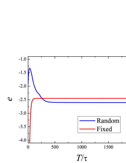
Figure 3: The energy value $e$ as a function of the time $T/\tau$ in the two cases of the initial random tensors and the initial fixed tensors whose components are all 1 for the system of $t=1$, $U=4$, $\mu=1$, $\chi=2$, $\kappa=2$, $L=10$, $\tau=0.02$, and $\xi=0.03$. We let the initial value of $e$ be zero, and we find that $e$ remains unchanged after $T/\tau=1774$ for $\mbox{seed}=7733$ and $T/\tau=255$ for no seed. Thus, we obtain the ground-state energy per site $e=-2.60549$ for the initial random tensors, and $e=-2.45054$ for the initial fixed tensors.

Because it is reasonable that the converging energy value is independent of any initial state, we should obtain the same ground-state energy up to the Suzuki-Trotter uncertainty $\tau^{2}$ as long as $t$, $U$ and $\mu$ are fixed. However, it seems that there are some barriers in the Hilbert space that prevent the evolving state from accessing the true ground state. In other words, if the initial state begins from a topologically different sector, it will never approach the true ground state in the process of TEBD. For example, in Fig. 3, we find the difference between the two converging energy values for the initial random tensors and the initial tensors whose components are fixed as 1. Thus, in further calculations, we should repeat simulations with several seed numbers to study the ground-state degeneracy and the disjoint space of tensor network states.

By changing the other parameters $t$, $U$, $\mu$, $\chi$, $\kappa$, and $L$, we can further verify the consistency. It is obvious that the ground-state energy $e$ should become twice as large when we simultaneously double $t$, $U$, and $\mu$. We have checked this consistency so that we can fix the value of $t$ as usual as $1$. Because the exact ground-state energy for the non-interacting infinite system [42] is known as $-1.6211$, we can compare the exact value to our value of $-1.3422$ for $\chi=\kappa=2$ in the system of $t=1$, $U=0$, $\mu=0$, and $L=10$. Furthermore, there is another exact result of the ground-state energy $-1.8514$ at $t=1$, $U=4$, $\mu=0$, and $L=4$ [43]. We compare it to our result of $-1.6508$ for $\chi=\kappa=2$ and $-1.6539$ for $\chi=\kappa=3$. Because of the finite values of $\chi$ and $\kappa$, there are some differences between the exact and ours. We find a tendency for our value to more closely approach the exact value as we increase $\chi$. However, the difference of $0.2$ is not small, and increasing $\chi$ may not improve the ground-state energy significantly. It indicates that the tensor network state in Fig. 2 may be incorrect.

In order to find the finite size effect related to $L$, we calculate the ground-state energy for the Hamiltonian of $t=1$, $U=4$ and $\mu=0$ by changing $L$. To save computing time, we perform the calculation for only the easy case of $\chi=\kappa=2$. We summarize the numerical results for various values of $L$ in Fig. 4 where we observe the saturation at large $L$.

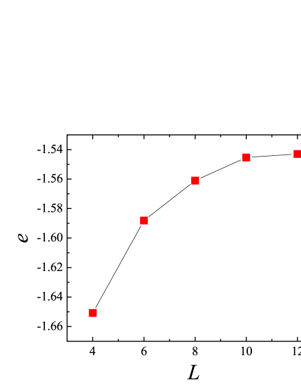
Figure 4: The plot of $e$ versus $L$ for the system of $t=1$, $U=4$, $\mu=0$, $\chi=2$, $\kappa=2$, $\tau=0.02$, and $\xi=0.03$. We note the saturation in the limit of $L\rightarrow\infty$.

Because the spin-flip symmetry preserving states in Eq. (6) are living in the subset of the Hilbert space for the spin-flip symmetry breaking states in Eq. (5), the converging energy for the state of Eq. (6) should be greater than or equal to the energy for the state of Eq. (5). For the spin-flip symmetry preserving states, in the process of TEBD, we perform updating the tensors and vectors in the spin-up layer, and then we duplicate the tensors and vectors in the spin-down layer from those in the spin-up layer. Because we duplicate the bonds in the spin-down layer, we should modify the factor $F$ such as $F~{}*=\lambda_{0}^{2}$ in the process of the horizontal and vertical bonds updating. We present the numerical results at $\mu=0$ in Fig. 5, comparing the ground-state energy of the spin-flip symmetry preserving state with that of the spin-flip symmetry breaking state. We note that the ground-state energy of the spin-flip symmetry preserving state is slightly lower than that of the spin-flip symmetry breaking state at small $U$. This is caused by numerical uncertainties, and it is understood as equality. This means that the symmetry breaking does not take place yet. We find from Fig. 5 that there is a transition at $U=0.39(1)$ for $\mu=0$. At large $U$, the ground-state energy of the spin-flip symmetry breaking state depends heavily on $U$. We note that the ground-state energy of the symmetry preserving state is almost independent of $U$. This independence means that the expectation value of the number operator is given by $\langle n_{i\uparrow}\rangle=\langle n_{i\downarrow}\rangle\approx\frac{1}{2}$ for any $i$.

We conclude that our method is effective in searching for the ground state of the Hubbard model. We emphasize that it is possible to determine the energy and the ground state for any chemical potential.

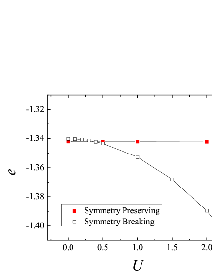
Figure 5: The ground-state energy $e$ versus $U$ for the system of $t=1$, $\mu=0$, $\chi=2$, $\kappa=2$, $L=10$, $\tau=0.02$, and $\xi=0.03$ with respect to the spin-flip symmetry breaking state of Eq. (5) and the spin-flip symmetry preserving state of Eq. (6). At small $U$, the ground-state energy for the state of Eq. (6) is roughly the same as that for the state of Eq. (5). We find a cut-point at $U=0.39(1)$. This is a signal of phase transition that takes place at $U=0.39(1)$ for $\mu=0$. For large $U$, the spin-flip symmetry breaking state is the true ground state in the model.

5 Conclusion

In summary, we have presented a method for obtaining the ground-state energy and the wave function for two-dimensional quantum many-fermion systems, especially the Hubbard model. We may call this method diffusive TEBD. Because there is a certain discrepancy between the exact ground-state energy and our value for the TNS, it is still questionable whether or not the TNS is correct and the diffusive TEBD is useful. We suggest that the diffusive TEBD is an effective method.

Although we built a user-friendly library in the framework of previous computer code [44], we obtain only preliminary numerical results because we use the full SVD, which is very inefficient. In future work, we will implement an SVD package based on the Lanczos algorithm with partial reorthogonalization [45] to find only a few eigenvectors and their corresponding singular values, which are sufficient for our truncation scheme.

When we use multi-core computers, it is possible to parallelize the local updates of the horizontal bonds and the spin bonds. For the vertical-bond update, we may apply the concept of a pipeline to optimize the roles of the multiple cores. We anticipate progress in this parallel computing scheme.

In future work, for a fixed $U$, we need to investigate whether any phase transitions happen as we change the chemical potential $\mu$ in the Hamiltonian. If there are any transitions in simulations, the phase transitions may be related to topological orders [46] or the topological entanglement entropy [47]. In connection with topological orders, we should give a definitive answer to the ground-state degeneracies. Furthermore, it is necessary to perform the same simulation by changing periodic or open boundary conditions.

It is of interest to extend our method to the case of two-body interactions. A typical topic of interest for two-body interactions may be the fractional quantum Hall effect, for which MPS can be used as an accessible subset of the huge Hilbert space. In the fractional quantum Hall effect, the energy gap between the ground state and the first excited state provides a lesser entanglement entropy, which makes it possible to use MPS with a relatively small bond dimension.

References

References

- [1] Gutzwiller M C 1963 Effect of Correlation on the Ferromagnetism of Transition Metals Phys. Rev. Lett. 10 159
- [2] Kanamori J 1963 Electron Correlation and Ferromagnetism of Transition Metals Prog. Theor. Phys. 30 275
- [3] Hubbard J 1963 Electron Correlations in Narrow Energy Bands Proc. R. Soc. A 276 238
- [4] Hubbard J 1964 Electron Correlations in Narrow Energy Bands. III. An Improved Solution Proc. R. Soc. A 281 401
- [5] Dagotto E 1994 Correlated electrons in high-temperature superconductors Rev. Mod. Phys. 66 763
- [6] Greiner M, Mandel O, Esslinger T, Hansch T W and Bloch I 2002 Quantum phase transition from a superfluid to a Mott insulator in a gas of ultracold atoms Nature 415 39
- [7] Jördens R, Strohmaier N, Günter K, Moritz H and Esslinger T 2008 A Mott insulator of fermionic atoms in an optical lattice Nature 455 204
- [8] Troyer M and Wiese U J 2005 Computational Complexity and Fundamental Limitations to Fermionic Quantum Monte Carlo Simulations Phys. Rev. Lett. 94 170201
- [9] Wilson K G and Kogut J 1974 The renormalization group and the expansion Phys. Rep. 12 75
- [10] Wilson K G 1975 The renormalization group: Critical phenomena and the Kondo problem Rev. Mod. Phys. 47 773
- [11] Kondo J 1964 Resistance Minimum in Dilute Magnetic Alloys Prog. Theor, Phys. 32 37
- [12] White S R 1992 Density matrix formulation for quantum renormalization groups Phys. Rev. Lett. 69 2863
- [13] Östlund S and Rommer S 1995 Thermodynamic Limit of Density Matrix Renormalization Phys. Rev. Lett. 75 3537
- [14] García-Ripoll J J 2006 Time evolution of Matrix Product States New J. Phys. 8 305
- [15] Saberi H, Weichselbaum A and von Delft J 2008 Matrix-product-state comparison of the numerical renormalization group and the variational formulation of the density-matrix renormalization group Phys. Rev. B 78 035124
- [16] Schollwöck U 2011 The density-matrix renormalization group in the age of matrix product states Ann. Phys. 326 96
- [17] Pérez-García D, Verstraete F, Wolf M M and Cirac J I 2008 PEPS as unique ground states of local Hamiltonians Quant. Inf. Comp. 8 0650
- [18] Orús R 2012 Exploring corner transfer matrices and corner tensors for the classical simulation of quantum lattice systems Phys. Rev. B 85 205117
- [19] Murg V, Verstraete F, Legeza Ó and Noack R M 2010 Simulating strongly correlated quantum systems with tree tensor networks Phys. Rev. B 82 205105
- [20] Vidal G 2007 Entanglement Renormalization Phys. Rev. Lett. 99 220405
- [21] Chou C P, Pollmann F and Lee T K 2012 Matrix-product-based projected wave functions ansatz for quantum many-body ground states Phys. Rev. B 86 041105
- [22] Levin M and Nave C P 2007 Tensor Renormalization Group Approach to Two-Dimensional Classical Lattice Models Phys. Rev. Lett. 99 120601
- [23] Jiang H C, Weng Z Y and Xiang T 2008 Accurate Determination of Tensor Network State of Quantum Lattice Models in Two Dimensions Phys. Rev. Lett. 101 090603
- [24] Xie Z Y, Chen J, Qin M P, Zhu J W, Yang L P and Xiang T 2012 Coarse-graining renormalization by higher-order singular value decomposition Phys. Rev. B 86 045139
- [25] Vidal G 2003 Efficient Classical Simulation of Slightly Entangled Quantum Computations Phys. Rev. Lett. 91 147902
- [26] Vidal G 2004 Efficient simulation of one-dimensional quantum many-body systems Phys. Rev. Lett. 93 040502
- [27] Vidal G 2007 Classical Simulation of Infinite-Size Quantum Lattice Systems in One Spatial Dimension Phys. Rev. Lett. 98 070201
- [28] Barthel T, Pineda C and Eisert J 2009 Contraction of fermionic operator circuits and the simulation of strongly correlated fermions Phys. Rev. A 80 042333
- [29] Kraus C V, Schuch N, Verstraete F and Cirac J I 2010 Fermionic projected entangled pair states Phys. Rev. A 81 052338
- [30] Corboz P, Orús R, Bauer B and Vidal G 2010 Simulation of strongly correlated fermions in two spatial dimensions with fermionic projected entangled-pair states Phys. Rev. B 81 165104
- [31] Pižorn I and Verstraete F 2010 Fermionic implementation of projected entangled pair states algorithm Phys. Rev. B 81 245110
- [32] Corboz P, Jordan J and Vidal G 2010 Simulation of fermionic lattice models in two dimensions with projected entangled-pair states: Next-nearest neighbor Hamiltonians Phys. Rev. B 82 245119
- [33] Corboz P, White S R, Vidal G and Troyer M 2011 Stripes in the two-dimensional t-J model with infinite projected entangled-pair states Phys. Rev. B 84 041108
- [34] Pineda C, Barthel T and Eisert J 2010 Unitary circuits for strongly correlated fermions Phys. Rev. A 81 050303
- [35] Corboz P and Vidal G 2009 Fermionic multiscale entanglement renormalization ansatz Phys. Rev. B 80 165129
- [36] Corboz P, Evenbly G, Verstraete F and Vidal G 2010 Simulation of interacting fermions with entanglement renormalization Phys. Rev. A 81 010303
- [37] Marti K H, Bauer B, Reiher M, Troyer M and Verstraete F 2010 Complete-graph tensor network states: a new fermionic wave function ansatz for molecules New J. Phys. 12 103008
- [38] Eisert J, Cramer M and Plenio M B 2010 Area laws for the entanglement entropy Rev. Mod. Phys. 82 277
- [39] Chung M H 2014 Diffusive time-evolving block decimation method for matrix product states in one-dimensional spinless fermion systems J. Korean Phys. Soc. 64 999
- [40] Ceperley D and Alder B 1986 Quantum Monte Carlo Science 231 555
- [41] Chung M H and Landau D P 2012 Diffusion Monte Carlo for fermions with replica reduction Phys. Rev. B 85 115115
- [42] Valentí R, Stolze J and Hirschfeld P J 1991 Lower bounds for the ground-state energies of the two-dimensional Hubbard and - models Phys. Rev. B 43 13743
- [43] Parola A, Sorella S, Baroni S, Parrinello M and Tosatti E 1989 Static properties of the 2D Hubbard model on a cluster Int. J. Mod. Phys. B 3 1865
- [44] Chung M H 2008 Science Code .Net: Object-oriented programming for science Sci. Comput. Program. 71 242
- [45] Simon H D 1984 The Lanczos algorithm with partial reorthogonalization Math. Comp. 42 115
- [46] Wen X G 1990 Topological Orders in Rigid States Int. J. Mod. Phys. B 4 239
- [47] Kitaev A and Preskill J 2006 Topological Entanglement Entropy Phys. Rev. Lett. 96, 110404