Formulation for zero mode of Bose-Einstein condensate beyond Bogoliubov approximation

Abstract

It is shown for the Bose-Einstein condensate of cold atomic system that the new unperturbed Hamiltonian, which includes not only the first and second powers of the zero mode operators but also the higher ones, determines a unique and stationary vacuum at zero temperature. From the standpoint of quantum field theory, it is done in a consistent manner that the canonical commutation relation of the field operator is kept. In this formulation, the condensate phase does not diffuse and is robust against the quantum fluctuation of the zero mode. The standard deviation for the phase operator depends on the condensed atom number with the exponent of $-1/3$, which is universal for both homogeneous and inhomogeneous systems.

I Introduction

Since the realization of Bose-Einstein condensate (BEC) in cold atomic systems Cornell ; Ketterle ; Bradley , it has been offering challenging subjects in theoretical foundations of quantum many-body problem. The theoretical description of BEC uses the complex order parameter or macroscopic wave function which is subject to the Gross-Pitaevskii (GP) equation, and is in very good agreement with the experiments at lower temperatures Dalfovo , as long as atomic interaction is weak and both quantum and thermal fluctuations can be neglected. The experimental observation of the interference between two condensates interference indicates that the order parameter of each condensate has a definite phase. The theoretical calculation based on the order parameter reproduces the interference fringe accurately Rohrl .

Quantum field theory, as the most fundamental one of quantum many-body problem, provides us with a clear and sound interpretation of the condensation: It is the ordered state associated with the spontaneous breakdown of the global gauge symmetry. At the same time the zero mode must exist according to the Nambu-Goldstone theorem NGtheorem1 ; NGtheorem2 , implying that it plays a crucial role in creating and retaining the ordered state. However, it is often, typically in the Bogoliubov approximation, neglected in formulating the quantum fluctuation at the sacrifice of the theoretical consistency. This is mainly because of its infrared singular property which is intractable and of a naive and groundless expectation that it does not affect the system very much. In this paper, we take full account of the zero mode from the standpoint of quantum field theory, in which the order parameter at zero temperature is given by the vacuum expectation of the field operator. The calculational scheme of quantum field theory is constructed in the interaction picture with an unperturbed Hamiltonian which contains the first and second powers of the field operator only but none of higher ones. Both of the zero and excitation modes on the condensate are described by the Bogoliubov-de Gennes (BdG) equation Bogoliubov ; deGennes ; Fetter , and the unperturbed field operator is expanded in the BdG complete set. While the unperturbed Hamiltonian of the excitation mode sector is diagonalized, that of the zero mode one is not Lewenstein ; Matsumoto2 ; Mine . Rather the dynamics of the zero mode should be represented by a pair of quantum coordinate $Q$ and momentum $P$, and the corresponding Hamiltonian is one of a free particle. Then the vacuum including the zero mode sector can not be determined for certain, because a stationary ground state does not exist. To overcome this problem, Lewenstein and You have introduced a new expansion of the field operator in which $Q$ becomes a phase operator of the condensate and concluded a phase diffusion, growing quadratically in time Lewenstein . We however note that their new field operator breaks the canonical commutation relation which is the very foundation of quantum field theory. Moreover, the predicted phase diffusion has not been observed experimentally, and several experiments are consistent with no phase diffusion Hall ; Greiner ; Gati . The treatment of the zero mode is still an open question.

In what follows, we consider a Bose–Einstein condensed system of weakly interacting atoms at zero temperature. Our proposition is that all the terms of the total Hamiltonian, consisting only of $Q$ and $P$, are taken in the unperturbed Hamiltonian. Then we naturally obtain a unique vacuum which is a stationary ground state of the zero mode sector and causes no infrared divergence, while the canonical commutation relation is not violated. We conclude from the evaluation of the variance in phase that no phase diffusion occurs and that the standard deviation of the phase decreases with the exponent $-1/3$ as the condensate number increases. It is shown that the exponent is universal and independent of whether the system is homogeneous or not.

II Ordinary Formulation and Dilemma of Zero Mode

Let us briefly sketch the ordinary formulation for the system at zero temperature, and see the dilemma of the zero mode mentioned above. We start with the total Hamiltonian,

$$H=\int\!d^{3}x\;\left[\psi^{\dagger}\left(-\frac{\nabla^{2}}{2m}+V_{\mathrm{ex}}-\mu\right)\psi+\frac{g}{2}\psi^{\dagger}\psi^{\dagger}\psi\psi\right]\,,$$ (1)

where $m$, $V_{\mathrm{ex}}$, $\mu$, and $g$ represent the mass of an atom, the confinement potential, the chemical potential, and the coupling constant, respectively, and $\hbar$ is set to be unity. The bosonic field operator $\psi$ obeys the canonical commutation relations ($x=({\bm{x}},t)$)

$$\bigl{[}\psi(x),\psi^{\dagger}(x^{\prime})\bigr{]}_{t=t^{\prime}}=\delta(\bm{x}-\bm{x}^{\prime})\,,\quad\bigl{[}\psi(x),\psi(x^{\prime})\bigr{]}_{t=t^{\prime}}=0\,,$$ (2)

and is divided into a classical part $\xi$ and an operator $\varphi$ on the criterion $\bigl{\langle}0\bigr{|}\varphi\bigl{|}0\bigr{\rangle}=0$. Note that the vacuum $\bigl{|}0\bigr{\rangle}$ is not specified yet and should be determined self-consistently. The total Hamiltonian is rewritten in terms of $\varphi$ as

$$H=H_{1}+H_{2}+H_{3}+H_{4}\,,$$ (3)

where

$$H_{1} =\int\!d^{3}x\;\left[(\varphi+\varphi^{\dagger})(h_{0}-\mu+g\xi^{2})\xi\right]\,,$$ (4)

$$H_{2} =\int\!d^{3}x\;\left[\varphi^{\dagger}\mathcal{L}\varphi+\frac{1}{2}\varphi\mathcal{M}\varphi+\frac{1}{2}\varphi^{\dagger}\mathcal{M}\varphi^{\dagger}\right]\,,$$ (5)

$$H_{3} =g\int\!d^{3}x\;\xi(\varphi^{\dagger}\varphi\varphi+\varphi^{\dagger}\varphi^{\dagger}\varphi)\,,$$ (6)

$$H_{4} =\frac{g}{2}\int\!d^{3}x\;\varphi^{\dagger}\varphi^{\dagger}\varphi\varphi\,,$$ (7)

with $h_{0}=-\nabla^{2}/2m+V_{\mathrm{ex}}\,,$ $\mathcal{L}=h_{0}-\mu+2g\xi^{2}\,,$ $\mathcal{M}=g\xi^{2}\,$. Here the order parameter $\xi$ is taken to be real for simplicity.

On the premise of small $\varphi$, the customary step is to choose $H_{1}+H_{2}$ as the unperturbed Hamiltonian except for the renormalization counter terms in the interaction picture. From $\bigl{\langle}0\bigr{|}\varphi\bigl{|}0\bigr{\rangle}=0$ for a time-independent vacuum $\bigl{|}0\bigr{\rangle}$ and any $t$ follows

$$i\partial_{t}\bigl{\langle}0\bigr{|}\varphi\bigl{|}0\bigr{\rangle}=\bigl{\langle}0\bigr{|}[\varphi,H_{1}+H_{2}]\bigl{|}0\bigr{\rangle}=0\,.$$ (8)

It implies $H_{1}=0$ and therefore the GP equation at the leading order GP ,

$$(h_{0}-\mu+g\xi^{2})\xi=0\,.$$ (9)

In an attempt to diagonalize $H_{2}$ Lewenstein ; Matsumoto2 ; Mine , we introduce the BdG equation $T\bm{y}_{\ell}=\omega_{\ell}\bm{y}_{\ell}\,$ with the doublet notations,

$$T=\begin{pmatrix}\mathcal{L}&\mathcal{M}\\ -\mathcal{M}&-\mathcal{L}\end{pmatrix}\,,\qquad\bm{y}_{\ell}=\begin{pmatrix}u_{\ell}\\ v_{\ell}\end{pmatrix}\,.$$ (10)

Due to the non-hermiticity of $T$, $\omega_{\ell}$ can be complex in general. The diagonalization of the complex mode part is also a subject to be settled Mine2007 . We restrict ourselves only to the real eigenvalues below. Because the global phase symmetry is spontaneously broken, there is a eigenfunction belonging to a zero eigenvalue, i.e. $T\bm{y}_{0}=0\,$ with $\bm{y}_{0}=(\xi,\;-\xi)^{t}\,$, and an additional adjoint function $\bm{y}_{-1}=(\eta,\;\eta)^{t}$ has to be introduced for the completeness, where $\eta=\frac{\partial\xi}{\partial N_{0}}$ and $N_{0}=\int\!d^{3}x\;\xi^{2}\,$. We adopt the following linear expansion of $\varphi(x)$ by the BdG complete set,

$$\varphi(x) =-iQ(t)\xi(\bm{x})+P(t)\eta(\bm{x})+\varphi_{\mathrm{ex}}(x)\,,$$ (11)

$$\varphi_{\mathrm{ex}}(x) =\sum_{\ell}\left[a_{\ell}(t)u_{\ell}(\bm{x})+a_{\ell}^{\dagger}(t)v_{\ell}^{*}(\bm{x})\right]\,.$$ (12)

The first two terms in Eq. (11) correspond to the zero mode part, while $\varphi_{\mathrm{ex}}$ represents the excited modes. The commutation relation of $\varphi$ leads us to

$$[Q(t),P(t)]=i\,,\quad[a_{\ell}(t),a_{\ell^{\prime}}^{\dagger}(t)]=\delta_{\ell\ell^{\prime}}\,,$$ (13)

and the vanishing ones otherwise, where $Q(t)$ and $P(t)$ are hermitian. Substituting the expansion (11) to Eq. (5), we obtain

$$H_{2}=\frac{IP^{2}}{2}+\sum_{\ell}\omega_{\ell}a_{\ell}^{\dagger}a_{\ell}\,,$$ (14)

where $I=\partial\mu/\partial N_{0}$. Thus the unperturbed Hamiltonian is diagonalized except for the zero mode part, which involves the fatal dilemma in choosing the vacuum. If one chooses the zero momentum state with the least eigenvalue as the vacuum, one has $\bigl{\langle}0\bigr{|}P^{2}(t)\bigl{|}0\bigr{\rangle}=0\,$, and the uncertainty relation implies $\bigl{\langle}0\bigr{|}Q^{2}(t)\bigl{|}0\bigr{\rangle}=\infty\,$, which is inconsistent with the assumption of the small $\varphi$. In general, one may choose a wave packet state with finite $\bigl{\langle}0\bigr{|}P^{2}(0)\bigl{|}0\bigr{\rangle}\,$ at $t=0$ as the vacuum, but the Heisenberg equation gives $Q(t)=Q(0)+IP(0)t$ and $\bigl{\langle}0\bigr{|}Q^{2}(t)\bigl{|}0\bigr{\rangle}$ grows as $t^{2}\,$. It shows that the choice of the wave packet is inadequate, or that it is valid only for a short time. Moreover, note that the unperturbed total atom number $\int\!d^{3}x\;\!\bigl{\langle}0\bigr{|}\psi^{\dagger}\psi\bigl{|}0\bigr{\rangle}$ also grows as $t^{2}\,$. To avoid the difficulties, Lewenstein and You have introduced a new expression of $\varphi(x)$ Lewenstein ,

$$\psi_{\rm LY}\equiv\bigl{(}\xi+\eta P+\varphi_{\mathrm{ex}}\bigr{)}e^{-iQ}\simeq\xi-iQ\xi+P\eta+\varphi_{\mathrm{ex}}\,,$$ (15)

where the last approximate expression is true only for small $Q$. Then the conservation of the total atomic number is recovered for the short time duration. However, we emphasize that because $\psi_{\rm LY}$ violates the canonical commutation relations which is the foundation of the quantum field theory, the formulation of quantum field theory in the interaction picture as a whole becomes unfounded.

III Treatment of Zero Mode Beyond Bogoliubov Approximation

The discussions above indicate that the simultaneous assumptions of the linear expansion of $\varphi$, the bilinear unperturbed Hamiltonian and small $\varphi$, are incompatible in treating the inevitable zero mode. We lift the choice of the unperturbed Hamiltonian, keeping the linear expansion and small $\varphi$, and instead include the terms with the third and forth order powers of the zero mode operators into the unperturbed Hamiltonian $H_{u}$ as follows:

$$H_{u}=H_{1}+H_{2}+\left[H_{3}+H_{4}\right]_{QP}-\delta\mu P\,,$$ (16)

where the symbol $\left[\cdots\right]_{QP}$ represents to pick up all the terms consisting only of the zero mode operators $Q$ and $P$, and the coefficient of the counter term $\delta\mu$ will be determined later. The remaining terms, e.g. the terms such as $a^{4}$ or $Pa^{\dagger}a$, are put into the interaction Hamiltonian. It is stressed that the canonical commutation relations are respected because the temporal evolution of $Q(t)$ and $P(t)$ are unitary, such as $Q(t)=e^{iH_{u}t}Q(0)e^{-iH_{u}t}\,$.

Substituting the expansion (11) into Eq. (16), we gather it as $H_{u}=H_{u}^{QP}+H_{u}^{\mathrm{ex}}\,$ with

$$H_{u}^{QP} =(2J-\mu+2B-\delta\mu-4C)P+\frac{I-4D}{2}P^{2}$$

$$\hskip 14.22636pt+2BQPQ+2DP^{3}+\frac{1}{2}AQ^{4}-2BQ^{2}$$

$$\hskip 28.45274pt+CQP^{2}Q+\frac{1}{2}EP^{4}\,,$$ (17)

$$H_{u}^{\mathrm{ex}} =\int\!d^{3}x\;(\varphi_{\mathrm{ex}}+\varphi_{\mathrm{ex}}^{\dagger})(h_{0}-\mu+g\xi^{2})\xi+\sum_{\ell}\omega_{\ell}a_{\ell}^{\dagger}a_{\ell}\,,$$ (18)

where

$$A =g\int\!d^{3}x\;\xi^{4}\,,\;\; B =g\int\!d^{3}x\;\xi^{3}\eta\,,\;\; C =g\int\!d^{3}x\;\xi^{2}\eta^{2}\,,\;\;$$

$$D =g\int\!d^{3}x\;\xi\eta^{3}\,,\;\; E =g\int\!d^{3}x\;\eta^{4}\,,\;\;$$

$$I =\frac{\partial\mu}{\partial N_{0}}\,,\;\; J =\int\!d^{3}x\;\eta h_{0}\xi\,.$$ (19)

Since $H_{u}$ contains no cross-term between $\{Q,P\}$ and $\varphi_{\mathrm{ex}}$, the whole unperturbed vacuum $\bigl{|}0\bigr{\rangle}$ is expressed as the direct product $\bigl{|}0\bigr{\rangle}=\bigl{|}\Psi\bigr{\rangle}\otimes\bigl{|}0\bigr{\rangle}_{\mathrm{ex}}$ where $\bigl{|}\Psi\bigr{\rangle}$ and $\bigl{|}0\bigr{\rangle}_{\mathrm{ex}}$ are vacua of the zero mode and excited mode sectors, respectively. The criterion of division $\bigl{\langle}0\bigr{|}\varphi\bigl{|}0\bigr{\rangle}=0$ leads

$${\!\!\phantom{\big{\langle}}}_{\mathrm{ex}}\bigl{\langle}0\bigr{|}\varphi_{\mathrm{ex}}\bigl{|}0\bigr{\rangle}_{\mathrm{ex}}=0\,,\quad\bigl{\langle}\Psi\bigr{|}Q\bigl{|}\Psi\bigr{\rangle}=0\,,\quad\bigl{\langle}\Psi\bigr{|}P\bigl{|}\Psi\bigr{\rangle}=0\,.$$ (20)

The time derivative of the first equality, in the same manner as in Eq. (8), derives the GP equation (9), which implies $2J-\mu+2B=0$ . The zero mode part of the unperturbed Hamiltonian $H_{u}^{QP}$ then becomes

$$H_{u}^{QP} =-(\delta\mu+4C)P+\frac{I-4D}{2}P^{2}+2BQPQ+2DP^{3}$$

$$+\frac{1}{2}AQ^{4}-2BQ^{2}+CQP^{2}Q+\frac{1}{2}EP^{4}\,.$$ (21)

Similarly, the time derivative of the second equality in Eq. (20) derives the identity

$$\bigl{\langle}\Psi\bigr{|}\bigl{[}-\delta\mu-4C+(I-4D)P+2BQ^{2}$$

$$\hskip 42.67912pt+6DP^{2}+2CQPQ+2EP^{3}\bigr{]}\bigl{|}\Psi\bigr{\rangle}=0\,,$$ (22)

which fixes $\delta\mu$ as

$$\delta\mu=\bigl{\langle}\Psi\bigr{|}\bigl{[}-4C+2BQ^{2}+6DP^{2}+2CQPQ+2EP^{3}\bigr{]}\bigl{|}\Psi\bigr{\rangle}\,,$$ (23)

to satisfy the third equality in Eq. (20). Here, the vacuum of the zero mode $\bigl{|}\Psi\bigr{\rangle}$ should be the ground state of the stationary Schrödinger equation,

$$H_{u}^{QP}\bigl{|}\Psi\bigr{\rangle}=E_{0}\bigl{|}\Psi\bigr{\rangle}\,,$$ (24)

and $\delta\mu$ is to be determined self-consistently. As there are terms with odd powers of $P$ but not of $Q$ in $H_{u}^{QP}$, the second equality in Eq. (20) is satisfied automatically when $\bigl{\langle}q\big{|}\Psi\bigr{\rangle}$ is an even function of $q$.

III.1 Variational Estimation for Homogeneous System

We first estimate $\bigl{|}\Psi\bigr{\rangle}$ variationally with the trial function,

$$\bigl{\langle}q\big{|}\Psi\bigr{\rangle}=\left(\frac{1}{2\pi\alpha^{2}}\right)^{1/4}e^{-\frac{q^{2}}{4\alpha^{2}}}\,.$$ (25)

The variational parameter $\alpha$ is related to the expectation value of $Q^{2}$ as $\alpha^{2}=\bigl{\langle}\Psi\bigr{|}Q^{2}\bigl{|}\Psi\bigr{\rangle}$. From Eq. (23), $\delta\mu$ is also expressed in terms of $\alpha$ as $\delta\mu=2B\alpha^{2}-4C+3D/2\alpha^{2}\,$. The parameter $\alpha$ is determined to minimize the expectation value $f(\alpha)=\bigl{\langle}\Psi\bigr{|}H_{u}^{QP}\bigl{|}\Psi\bigr{\rangle}\,$, that is

$$\frac{\partial f}{\partial\alpha}=6A\alpha^{3}-4B\alpha^{2}-\frac{I-4D}{4\alpha^{3}}-\frac{3E}{8\alpha^{5}}=0\,.$$ (26)

In the large $N_{0}$ limit, only the terms proportional to $A$ and $I$ are dominant in Eq. (26), and we obtain

$$\alpha=\sqrt[6]{\frac{I}{24A}}\,.$$ (27)

When we consider a homogeneous system ($V_{\mathrm{ex}}=0$ and $\xi=$ constant) where $\xi=N_{0}/V\,,\mu=gN_{0}/V\,,$ and $I=g/V$ with the volume $V$, Eq. (27) leads to $\alpha=(1/{\sqrt[6]{24}})\,N_{0}^{-1/3}$. It is independent of both $g$ and $V$, and depends only on $N_{0}$. The standard deviation of $Q$, denoted by $\Delta Q=\sqrt{\bigl{\langle}\Psi\bigr{|}Q^{2}\bigl{|}\Psi\bigr{\rangle}-\bigl{\langle}\Psi\bigr{|}Q{\bigl{|}\Psi\bigr{\rangle}}^{2}}$, is equal to $\alpha$ since $\bigl{\langle}\Psi\bigr{|}Q\bigl{|}\Psi\bigr{\rangle}=0$ for the trial function (25). As long as $\Delta Q$ is sufficiently small, it is interpreted as the fluctuation of the phase, $\psi\simeq\xi-iQ\xi+\cdots\simeq e^{-iQ}\xi+\cdots$, similarly as in Eq. (15) which is not adopted in our approach though. Our estimation of Eq. (27) shows that the uncertainty of the condensate phase decreases as $N_{0}^{-1/3}$, and vanishes at the thermodynamical limit.

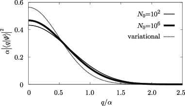
Figure 1: The ground state distribution for the homogeneous system. The thin and bold lines denote the numerical results for $N_{0}=10^{2}$ and $10^{6}$, respectively. For comparison the variational result is shown as the dotted line. As the axes are scaled by $\alpha$, the dotted line is true for an arbitrary $N_{0}$.

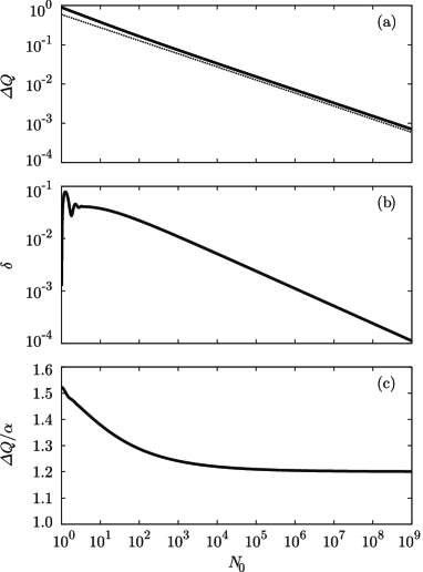
Figure 2: $N_{0}$ dependences of (a) $\Delta Q$, (b) $\delta$, and (c) $\Delta Q/\alpha$ for the homogeneous system. The dotted line in (a) indicates the variational estimation $\alpha=(1/\sqrt[6]{24})N_{0}^{-1/3}$. The quality $\delta=-1/3-\frac{d\log\Delta Q}{d\log N_{0}}$ in (b) indicates the shift of the exponent of $\Delta Q$ from $-1/3$.

III.2 Numerical Calculation for Homogeneous System

We next solve Eq. (24) numerically for the homogeneous system. The numerical results of the ground state distribution is depicted in Fig. 1, and allow us to calculate $\Delta Q\,$. Figure 2 (a) shows that the variational estimation ($\alpha$, dotted line) is in good agreement with the numerical result ($\Delta Q$, solid line). Let us introduce the quantity $\delta$ by parameterizing $\Delta Q\sim N_{0}^{-(1/3+\delta)}$. As shown in Fig. 2 (b), $\delta$ decreases exponentially for large $N_{0}$ and implies that the exponent converges to $-1/3$ in the limit $N_{0}\to\infty\,$, as is estimated variationally. Unlike in the case of the exponent, the coefficient in $\Delta Q$ differs from the variational estimation, and the ratio $\Delta Q/\alpha$ converges to about $1.20$ as Fig. 2 (c) shows. It is not negligible small but one may conclude that the variational estimation is valid.

III.3 Inhomogeneous System

Finally, we confirm that the behavior of $\Delta Q\sim N_{0}^{-1/3}$ for large $N_{0}$ is universal even for an inhomogeneous system with $V_{\mathrm{ex}}(\bm{x})\neq 0$ and is independent of the interaction strength, dimension, and the shape of the confinement potential. We consider a $d$-dimensional system with a repulsive interaction $g>0\,$, and the attractive case is excluded because then the condensate collapses for large $N_{0}$. Let us suppose that $V_{\mathrm{ex}}(\bm{x})$ has a form of homogeneous function: $V_{\mathrm{ex}}(\lambda\bm{x})=\lambda^{\nu}V_{\mathrm{ex}}(\bm{x})$ with a parameter $\nu\geq 1$. Then the virial theorem yields PethickSmith the relation $2E_{\mathrm{kin}}-\nu E_{\mathrm{pot}}+dE_{\mathrm{int}}=0$, where $E_{\mathrm{kin}}=\frac{1}{2m}\int\!d^{d}x\,\left|\nabla\xi(\bm{x})\right|^{2}$ , $E_{\mathrm{pot}}=\int\!d^{d}x\,V_{\mathrm{ex}}(\bm{x})\left|\xi(\bm{x})\right|^{2}$ , and $E_{\mathrm{int}}=\frac{g}{2}\int\!d^{d}x\,\left|\xi(\bm{x})\right|^{4}$ . Besides, one derives $E_{\mathrm{kin}}+E_{\mathrm{pot}}+2E_{\mathrm{int}}=\mu N_{0}$ from the Gross-Pitaevskii equation. Taking the large $N_{0}$ limit and using the Thomas–Fermi approximation, $E_{\mathrm{kin}}=0$, we obtain $\mu=E_{\mathrm{int}}(d+2\nu)/\nu N_{0}$. The interaction energy $E_{\mathrm{int}}$ is equal to $A/2$ [see Eq.(III)], and its leading term in the large $N_{0}$ limit can be expressed as $A\simeq c_{1}N_{0}^{c_{2}}$ with $c_{1}>0$ and $c_{2}>1$. Using Eqs. (III) and (27), we obtain

$$\Delta Q=\sqrt[6]{\frac{(d+2\nu)(c_{2}-1)}{48\nu}}N_{0}^{-1/3}\,,$$ (28)

where the power of $N_{0}$ is independent of the other parameters and equals to $-1/3$.

IV Summary

In summary, including the terms with higher powers of the zero mode operators $Q$ and $P$ in the unperturbed Hamiltonian, we have obtained the appropriate vacuum which is stationary and whose validity is not restricted to a finite time duration. This is a contrast to the previous theoretical formulation in which no discrete ground state exist and the phase of the order parameter diffuses out. The difference comes simply from the choices of the unperturbed Hamiltonian in both the cases. We have evaluated the standard variation $\Delta Q$ which is interpreted as the condensate phase when $\Delta Q\ll 1$. The phase fluctuation $\Delta Q$ decreases as $\sim N_{0}^{-1/3}$ for large $N_{0}$. This power law is universal and independent of the other parameters for the both homogeneous and inhomogeneous systems. We note that while the power law is independent of the interaction constant $g$, the presence of non-zero $g$ is crucial to the robustness of the condensate phase against the quantum fluctuation of the zero mode. If the higher powers of the zero mode operators, i.e. $[H_{3}+H_{4}]_{QP}$, are excluded from the unperturbed Hamiltonian, the present formulation reduces to that of Lewenstein and You Lewenstein . The higher power contribution of the zero mode operators is essential to go beyond Bogoliubov approximation and to determine a unique stationary vacuum. In this paper, we have considered only the case where the quantum fluctuation of the exited modes and the thermal one of all the modes are negligibly small. To extend the present formulation to a system at finite temperature would be the future work.

- (1) M. H. Anderson, J. R. Ensher, M. R. Matthews, C. E. Wieman, and E. A. Cornell, Science 269, 198 (1995).
- (2) K. B. Davis, M.-O. Mewes, M. R. Andrews, N. J. van Druten, D. S. Durfee, D. M. Kurn, and W. Ketterle, Phys. Rev. Lett. 75, 3969 (1995).
- (3) C. C. Bradley, C. A. Sackett, J. J. Tollett, and R. G. Hulet, Phys. Rev. Lett. 75, 1687 (1995).
- (4) F. Dalfovo, S. Giorgini, L. P. Pitaevskii, and S. Stringari, Rev. Mod. Phys. 71, 463 (1999).
- (5) M. R. Andrews, C. G. Townsend, H.-J. Miesner, D. S. Durfee, D. M. Kurn, and W. Ketterle, Science 275, 637 (1997).
- (6) A. Röhrl, M. Naraschewski, A. Schenzle, and H. Wallis, Phys. Rev. Lett. 78, 4143 (1997).
- (7) J. Goldstone, Nuovo Cimento 19, 154 (1961).
- (8) Y. Nambu and G. Yona-Lasinio, Phys. Rev. 122, 345 (1961).
- (9) N. N. Bogoliubov, J. Phys. (Moscow) 11, 32 (1947).
- (10) P. G. de Gennes, Superconductivity of Metals and Alloys (Benjamin, New York, 1966).
- (11) A. L. Fetter, Ann. Phys. (N.Y.) 70, 67 (1972).
- (12) M. Lewenstein and L. You, Phys. Rev. Lett. 77, 3489 (1996).
- (13) H. Matsumoto and S. Sakamoto, Prog. Theor. Phys. 107, 679 (2002).
- (14) M. Mine, M. Okumura, and Y. Yamanaka, J. Math. Phys. 46, 042307 (2005).
- (15) D. S. Hall, M. R. Matthews, C. E. Wieman, and E. A. Cornell, Phys. Rev. Lett. 81, 1543 (1998).
- (16) M. Greiner, O. Mandel, T. Esslinger, T. W. Hänsch, and I. Bloch, Nature 415, 39 (2002).
- (17) R. Gati, B. Hemmerling, J. Fölling, M. Albiez, and M. K. Oberthaler Phys. Rev. Lett. 96, 130404 (2006).
- (18) E. P. Gross, Nuovo Cimento 20, 454 (1961); J. Math. Phys. 4, 195 (1963). L. P. Pitaevskii, Zh. Eksp. Teor. Fiz. [Soc. Phys. JETP] 40, 546 (1961); Sov. Phys. JETP 13, 451 (1961).
- (19) M. Mine, M. Okumura, T. Sunaga, and Y. Yamanaka, Ann. Phys. (N.Y.) 322, 2327 (2007).
- (20) C. J. Pethick and H. Smith, Bose–Einstein Condensation in Dilute Gases (Cambridge University Press, Cambridge, 2008).