Statistics and Classification of the Microwave Zebra Patterns Associated with Solar Flares

Abstract

The microwave zebra pattern (ZP) is the most interesting, intriguing, and complex spectral structure frequently observed in solar flares. A comprehensive statistical study will certainly help us to understand the formation mechanism, which is not exactly clear now. This work presents a comprehensive statistical analysis on a big sample with 202 ZP events collected from observations at the Chinese Solar Broadband Radio Spectrometer at Huairou and the Ondŕejov Radiospectrograph in Czech Republic at frequencies of 1.00 - 7.60 GHz during 2000 - 2013. After investigating the parameter properties of ZPs, such as the occurrence in flare phase, frequency range, polarization degree, duration, etc., we find that the variation of zebra stripe frequency separation with respect to frequency is the best indicator for a physical classification of ZPs. Microwave ZPs can be classified into 3 types: equidistant ZP, variable-distant ZP, and growing-distant ZP, possibly corresponding to mechanisms of Bernstein wave model, whistler wave model, and double plasma resonance model, respectively. This statistical classification may help us to clarify the controversies between the existing various theoretical models, and understand the physical processes in the source regions.

1 Introduction

As we have known, zebra pattern (ZP) is a kind of spectral fine structure superposed on the solar radio broadband type IV continuum spectrogram, which consists of several almost parallel and equidistant stripes. It is the most intriguing and interesting fine structure on the dynamic spectra of solar radio observations, especially at microwave frequency range, which may reveal the original information of the solar flaring processes, such as the magnetic fields and its configurations, particle acceleration, and the plasma features in the source regions where the primary energy releases. The nature of ZP structures has been a widely discussed subject for more than 40 years. The historical development of observations and various theoretical models is assembled in the review of Chernov (2006), Zlotnik (2009), and so on (Rosenberg 1972, Kuijpers 1975, Zheleznyakov & Zlotnik 1975, Chernov 1976, 1990, LaBelle et al. 2003, Kuznetsev 2005, Ledenev et al. 2006, Tan 2010, Karlicky 2013). These models include:

(1) Bernstein wave (BW) model

It is the first model interpreting the formation of ZP structure which proposed that all the stripes in a ZP structure are generated from a small compact source, and the emission produces from some nonlinear coupling processes between two Bernstein waves, or Bernstein wave and other electrostatic upper hybrid waves. The electrons with non-equilibrium distribution over velocities perpendicular to the magnetic field are located in a small source, where the plasma is weakly and uniformly magnetized ($f_{pe}\gg f_{ce}$). These electrons excite longitudinal electrostatic waves at frequency of the sum of Bernstein modes frequency $sf_{ce}$ and the upper hybrid frequency $f_{uh}$: $f=f_{uh}+sf_{ce}\approx f_{pe}+sf_{ce}$. Here, $f_{pe}$ is the electron plasma frequency, $f_{ce}$ the electron gyro-frequency, $s$ is harmonics number. The BW excitation occurs in relatively narrow frequency band. This model predicts the frequency separation between the adjacent zebra stripes just as the electron gyro-frequency: $\Delta f=f_{ce}$ (Rosenberg 1972, Chiuderi et al. 1973, Zheleznyakov & Zlotnik 1975, Zaitsev & Stepanov 1983), it approximates a constant.

(2) Whistler wave (WW) model

This is an important model based on propagation of whistler wave packets across or along the magnetic loop where the energetic electrons generate Langmuir waves (Kuijpers 1975, Chernov 1976, Maltseva & Chernov 1989). The quasi-standing whistler packets can be driven by loss-cone distribution of fast electrons in the entire magnetic trap at some cyclotron resonance conditions. The coupling of plasma Langmuir waves and whistler wave packets can operate in different resonance conditions: when whistlers generate at the normal Doppler cyclotron resonance they can escape along the magnetic loop and yield fiber bursts ($f_{w}-\frac{k_{\parallel}}{2\pi}v_{\parallel}-f_{ce}=0$, $f_{w}$ is the whistler wave frequency, $k_{\parallel}$ is the whistler wave number paralleled to magnetic field, $v_{\parallel}$ is the fast electron velocity paralleled to magnetic field); when whistlers generate at the anomalous Doppler cyclotron resonance ($f_{w}-\frac{k_{\parallel}}{2\pi}v_{\parallel}+f_{ce}=0$) under large angles to the magnetic field they may form standing wave packets in front of the shock wave, and when the group velocity of whistlers is approximated to the shock velocity, a ZP structure with slow oscillating frequency drift will appear. Each zebra stripe corresponds to one propagating whistler wave packet. The emission frequency at $f=f_{pe}+sf_{w}$, $f_{w}\approx 0.1-0.5f_{ce}$ is the whistler wave frequency. Here, $f_{pe}\gg f_{ce}$. The frequency separation $\Delta f$ of adjacent zebra stripes is about 2 times of whistler wave frequency: $\Delta f\sim 2f_{w}$. As $f_{w}$ varies in a small range, the whistler wave group velocity peaks at frequency of $\frac{1}{4}f_{ce}$, therefore, $\Delta f$ will vary around $\frac{1}{2}f_{ce}$.

(3) Double plasma resonance (DPR) model

The most developed heterogenous ZP model is called double plasma resonance model (DPR model), which proposed that enhanced excitation of plasma waves occurs at some resonance levels where the upper hybrid frequency coincides with the harmonics of electron gyro-frequency in the inhomogeneous flux tube (Pearlstein et al. 1966, Zheleznyakov & Zlotnik 1975, Berney & Benz 1978, Winglee & Dulk 1986, Zlotnik et al. 2003, Yasnov & Karlicky 2004, Kuznetsov & Tsap 2007): $f_{uh}=(f_{pe}^{2}+f_{ce}^{2})^{1/2}=sf_{ce}$. The emission frequency is dominated not only by the electron gyro-frequency, but also by plasma frequency. When the emission generates from the coalescence of two excited plasma waves, the polarization may be very weak, the emission frequency is $f\approx 2f_{pe}\approx 2sf_{ce}$, and the stripe frequency separation is $\Delta f=\frac{2sf_{ce}H_{b}}{|sH_{b}-(s+1)H_{p}|}$. Here, $H_{b}$ and $H_{p}$ are the scale heights of magnetic field and the plasma density in the source regions, respectively. When the emission generates from the coalescence of an excited plasma wave and a low frequency electrostatic wave, the polarization will be strong, the emission frequency is $f\approx f_{pe}\approx sf_{ce}$, and the stripe frequency separation is $\Delta f=\frac{sf_{ce}H_{b}}{|sH_{b}-(s+1)H_{p}|}$. In DPR model, $\Delta f$ has a regular changing trend with a fairly large number of stripes. Here, $\Delta f$ depends on $H_{b}$ and $H_{p}$, which therein depends on the models of coronal magnetic field and plasma density. For most models, we can deduce that $\Delta f$ will increase with respect to the frequency.

(4) Propagating model

There are also some models proposed that ZP stripes could be formed in the propagating processes after emitted from source regions. The interference model suggests that ZP is formed from some interference mechanisms in the propagating processes (Bárta & Karlický 2006, Ledenev et al. 2006). Some inhomogeneous layers with small size may appear in source region, they can change the emission into direct and reflected rays. When the direct and reflected rays meet at some places, interference will take place and produce ZP. This model needs a structure with great number of discrete sources in small size, such structure may exist in the current-carrying flaring plasma loop (Tan 2010) where the tearing-mode instability forms a great number of magnetic islands which may provide the main conditions for the interference mechanism, similar to the crystal lattice. Very recently, Karlicky (2013) proposed a new model that links ZP with propagating compressive MHD waves. However, so far, the propagating model is hard to predict the zebra stripe frequency separation, and the relationship between the zebra parameters and the magnetic field in the source region is also unknown.

Until now, the real formation of microwave ZPs is still controversial. It is very difficult to interpret all observing properties by using a unique existing model. It is meaningful to make a classification of microwave ZPs. Possibly, the different microwave ZPs may have different formation mechanism. Therefore, a comprehensive statistical analysis of microwave ZPs is most necessary.

In previous literatures, there are some statistical works on ZP structures (Huang et al. 2008, 2010, Huang & Tan 2012, Yu et al. 2012), but a physical classification is still missing. This work will present a comprehensive statistical investigation on the microwave ZPs at frequency of above 1000 MHz. Section 2 introduces the observations and the composition of the statistical sample, section 3 presents the statistical properties of ZP parameters. A physical classification of ZPs is presented in section 4. Finally, some conclusions discussions are summarized in section 5.

2 Statistical Sample

2.1 Observation data

In this work, the statistical sample in obtained from the following two broadband solar radio spectrometers:

(1) The Chinese Solar Broadband Radio Spectrometers at Huairou (SBRS/Huairou)

SBRS is an advanced solar radio telescope with super high cadence, broad frequency bandwidth, and high frequency resolution, which can distinguish the super fine structures from the spectrogram (Fu et al. 1995, 2004, Yan et al. 2002). Its daily observational window is 0:00-8:00 UT in winter seasons and 23:00-9:00 UT in summer seasons. It includes 3 parts: 1.10 - 2.06 GHz (with the antenna diameter of 7.0 m), 2.60 - 3.80 GHz (with the antenna diameter of 3.2 m), and 5.20 - 7.60 GHz (share the same antenna of the second part). The antenna points to the center of solar disk automatically controlled by a computer. The spectrometer receives the total flux of solar radio emission with dual circular polarization (left- and right handed circular polarization, LCP and RCP), and the dynamic range is 10 dB above quiet solar background emission. The observation sensitivity is: $S/S_{\bigodot}\leq 2\%$, here $S_{\bigodot}$ is the quiet solar background emission. Our observation data includes:

During 2000-2003 and 2006-2008, 1.10-2.06 GHz with cadence of 5 ms and frequency resolution of 4 MHz;

During 2004 - 2005, 1.10 - 1.34 GHz with cadence of 1.25 ms and frequency resolution of 4 MHz;

During 2000 - 2013, 2.60 - 3.80 GHz with cadence of 8 ms and frequency resolution of 10 MHz;

During 2000 - 2008, 5.20 - 7.60 GHz with cadence of 5 ms and frequency resolution of 20 MHz.

(2) Ondŕejov radiospectrograph in Czech Republic (ORSC/Ondŕejov).

ORSC is another broadband spectrometer located at Ondŕejov, Czech republic. It can receive solar radio total flux at frequencies of 0.80 - 5.00 GHz during 2000 - 2013 (Jiricka et al. 1993). Its daily observational window is 7:00-16:00 UT in winter seasons and 6:00-17:00 UT in summer seasons. Our observation data includes:

During 2000 - 2005, 0.80 - 2.00 GHz with cadence of 100 ms and frequency resolution of 5 MHz; 2.00 - 4.50 GHz with cadence of 100 ms and frequency resolution of 10 MHz;

During 2006 - 2013, 0.80 - 2.00 GHz with cadence of 10 ms and frequency resolution of 5 MHz; 2.00 - 5.00 MHz with cadence of 100 ms and frequency resolution of 12 MHz.

SBRS/Huairou and ORSC/Ondŕejov have a overlapping observational window 7:00 - 8:00 UT in winter seasons and 6:00-9:00 UT in summer seasons.

2.2 Statistical Parameters

It is necessary to make a clear definition of a ZP event. Here we define a ZP event as an isolated spectral structure, which consists of at least 2 almost-parallel stripes with approximately equidistant separation and slowly frequency drifting rate, the time gap between two such adjacent similar ZP events is at least longer than the duration of each ZP event, and the frequency gap between two such adjacent similar ZP events is at least wider than the frequency range of each ZP event. Based on such definition, we find that some flares have only one ZP event, while some flares may accompany with several ZP events. By scrutinizing the broadband spectrograms, we find that there are 154 ZP events in 27 flares observed by SBRS, and 49 ZP events in 13 flares observed by ORSC during 2000 - 2013. There is only one ZP event observed simultaneously by SBRS and ORSC in an M6.5 flare on 2013 April 11. There are totally 202 ZP events in 40 flares, which are listed in Table 1.

Table 1: List of solar flares with microwave ZPs during 2000 - 2013

Date	Class	$t_{st}$(UT)	$t_{fp}$(UT)	$D_{ri}$(min)	phase	$N_{zp}$	$f_{zp}$	Telescope
2013-04-11	M6.5	06:58	07:16	18	rising	4	2.6-3.8	SBRS,ORSC
2012-06-13	M1.1	12:04	13:15	71	peak	3	1.3-1.8	ORSC
2011-08-09	X6.9	08:00	08:04	4	peak	1	2.6-3.8	SBRS
2011-02-24	M3.5	07:26	07:35	9	peak	2	2.6-3.8	SBRS
2011-02-15	X2.2	01:46	01:56	10	rising	1	5.2-7.6	SBRS
					decay	2	2.6-3.8	SBRS
2010-08-01	C3.2	07:55	09:00	65	rising	8	1.1-1.5	ORSC
2006-12-13	X3.4	02:14	02:40	26	rising	4	2.6-3.8	SBRS
					peak	1	2.6-3.8	SBRS
					decay	4	2.6-3.8	SBRS
2006-12-05	X9.0	10:18	10:35	17	rising	6	2.4-3.6	ORSC
2005-07-11	C1.0	16:33	16:37	4	decay	2	1.3-1.6	ORSC
2005-07-09	M2.8	21:47	22:06	19	rising	4	2.6-3.8	SBRS
2005-06-01	C2.3	10:41	10:51	10	rising	1	1.0-1.3	ORSC
2005-01-16	X2.6	22:25	23:02	37	decay	1	1.1-2.06	SBRS
2005-01-15	X1.2	00:22	00:43	21	peak	1	2.6-3.8	SBRS
2005-01-15	M8.6	05:54	06:37	43	rising	7	2.6-3.8, 1.1-1.34	SBRS
					peak	3	2.6-3.8, 1.1-1.34	SBRS
					decay	3	1.1-1.34	SBRS
2004-12-02	M1.5	23:44	00:06	22	rising	4	1.1-1.34	SBRS
2004-12-01	M1.1	07:00	07:20	20	rising	3	2.6-3.8, 1.1-1.34	SBRS
2004-11-10	X2.5	01:59	02:13	14	decay	1	2.6-3.8	SBRS
2004-10-30	M3.7	09:09	09:28	19	rising	2	2.1-3.4	ORSC
2004-10-30	C3.7	12:45	12:51	6	peak	1	2.1-2.4	ORSC
2004-09-12	M4.8	00:04	00:56	52	rising	9	2.6-3.8	SBRS
					peak	1	2.6-3.8	SBRS
2004-05-17	C7.0	04:11	04:17	6	peak	3	1.1-2.06	SBRS
2004-04-06	M2.4	12:30	13:28	58	peak	3	2.5-4.0	ORSC
2004-01-09	M1.1	01:13	01:22	9	peak	7	1.1-2.06	SBRS
2004-01-05	M6.9	02:50	03:45	55	rising	2	1.1-2.06	SBRS
2003-11-18	M3.9	08:12	08:31	19	rising	6	2.6-3.8	SBRS
2003-10-28	X17	11:00	11:10	10	decay	1	2.0-2.4	ORSC
2003-10-26	X1.2	05:57	06:54	57	rising	14	1.1-2.06	SBRS
2003-05-29	M1.5	02:09	02:18	9	rising	2	5.2-7.6	SBRS
2003-05-27	M1.6	05:06	06:26	80	rising	1	1.1-2.06	SBRS
					peak	12	1.1-2.06	SBRS
2003-03-18	X1.5	11:52	12:08	16	decay	1	2.0-2.4	ORSC
2003-01-05	C5.8	05:51	06:17	26	rising	2	5.2-7.6	SBRS
2002-09-17	C8.8	09:17	09:21	4	peak	5	2.0-4.5	ORSC
2002-04-21	X1.5	00:43	01:10	27	decay	12	2.6-3.8	SBRS
2001-10-19	X1.6	00:47	01:05	18	rising	5	2.6-3.8	SBRS
					decay	2	2.6-3.8	SBRS
2001-09-16	C4.3	07:40	07:45	5	rising	1	1.2-1.6	ORSC
2000-11-25	M8.2	00:59	01:31	32	rising	10	2.6-3.8	SBRS
2000-11-24	X2.0	04:55	05:02	7	rising	2	2.6-3.8	SBRS
					peak	2	2.6-3.8	SBRS
2000-10-29	M4.4	01:28	01:57	29	decay	14	2.6-3.8	SBRS
2000-06-06	X2.3	15:00	15:26	26	decay	14	2.0-3.5	ORSC
2000-04-09	M3.1	23:26	23:42	16	rising	1	2.6-3.8	SBRS
Sum	40 flares					202

Note. — $Class$: the GOES soft X-ray class, $t_{st}$: flare start time, $t_{fp}$: flare peak time, $D_{ri}$: flare rising time, $t_{zp}$: the central time of ZP; $f_{zp}$: frequency range of ZP (GHz); $N_{zp}$: number of ZP events in the flare. SBRS indicates the Chinese Solar Broadband Radio Spectrometers at Huairou, and ORSC indicates the Ondŕejov radiospectrograph in Czech Republic.

In order to investigate the relationship between ZP and the flaring processes, we define a phase time $P_{ph}$ to describe the relative time of ZP structure occurrence with respect to the maximum of solar flare:

$$P_{ph}=(t_{zp}-t_{fp})/(t_{fp}-t_{st}).$$ (1)

$t_{zp}$ is the central time of ZP structure. $t_{fp}$ and $t_{st}$ are the peak and start time of the GOES soft X-ray (SXR) flare, respectively. $t_{st}$ is defined when four consecutive 1 minutes SXR values have met all three of the following conditions: (1) all four values are above the background threshold, (2) all four values are strictly monotonically increasing, and (3) the last value is 1.4 times greater than the value occurred 3 minutes earlier. $D_{ri}=t_{fp}-t_{st}$ is the flare rising time. $P_{ph}=-1.00$ indicates the time at flare start, $P_{ph}=0$ indicates the flare maximum (peak time), and $P_{ph}>0$ indicates the time after the flare maximum. According to $P_{ph}$, the flaring process can be partitioned into three phases:

(1) Rising phase: $P_{ph}\leq-0.25$, SXR intensity is increasing rapidly. During this phase, the flaring region may undergo continuously magnetic flux emergence, reconnections, energy releasing, and plasma heating.

(2) Peak phase: $-0.25<P_{ph}\leq 0.25$, SXR intensity is relatively stable, and has only a slightly variation. During this phase, the magnetic flux emergence and the magnetic energy releasing in the flaring region may reach to a steady state.

(3) Decay phase: $P_{ph}>0.25$, SXR intensity is decreasing slowly and continuously. During this phase, besides some local small scale magnetic reconnections, the main energy releasing is ended, and the flaring region may undergo a process of thermal dissipations and cooling.

In left panel of Figure 1, the dotted curve is an example profile of GOES SXR emission in a typical flare, the vertical dashed lines partition flaring process into rising, peak, and decay phases.

Table 2: The parameters of microwave ZPs in a M8.6 flare on 2005 January 15

Phase	$t_{zp}$	$P_{ph}$	$N_{str}$	$f_{zp}$(MHZ)	$\Delta f$   (MHz)	$\Delta f/f_{zp}$(%)	$r(\%)$	$D_{zp}$   (s)
rising	06:13:10	-0.55	5	1204	28	2.33	100	0.5
	06:13:27	-0.54	5	1296	36	2.78	100	4.0
	06:14:58	-0.51	2	2680	100	3.73	0	5.0
	06:15:20	-0.50	5	1192	26	2.18	100	2.0
	06:16:32	-0.48	2	2730	90	3.30	0	3.0
	06:23:02	-0.32	5	1196	18	1.51	100	0.8
	06:24:34	-0.29	4	1196	20	1.67	100	3.5
peak	06:27:39	-0.22	3	2750	105	3.82	0	4.0
	06:28:36	-0.22	3	2750	120	4.36	0	4.5
	06:31:44	-0.12	6	1240	52	6.77	0	30.0
decay	06:49:10	0.28	5	1224	48	3.92	20	45.0
	06:51:07	0.33	9	1180	18	1.53	85	0.8
	07:17:32	1.18	8	1150	14	1.22	100	3.3

Note. — $t_{zp}$: central time (UT); $P_{ph}$: phase time, $f_{zp}$: central frequency; $\Delta f$: frequency separation of zebra stripes, $\Delta f/f_{zp}$: relative frequency separation, $N_{str}$: zebra stripe number, $D_{zp}$: ZP duration, $r$: averaged polarization degree.

Besides the phase time $P_{ph}$, we also collect the ZP central frequency ($f_{zp}$), stripe number ($N_{zp}$), frequency separation between adjacent zebra stripes ($\Delta f$), relative frequency separation ($\Delta f/f_{zp}$), averaged degree of polarization ($r$), and the ZP duration ($D_{zp}$). Table 2 lists the parameters of ZPs occurring in a long-duration flare. In this work, we measured all above parameters of each ZP event in the sample, which will be analyzed in the following sections.

3 Statistical Results and Analysis

Based on the above sample of 202 microwave ZP events, we present comprehensively statistical investigations in this section.

3.1 The ZP dependence with flares

At first, we hope to know which kind of flares and what phase of the flare may be preferential to produce ZP phenomena. Table 1 indicates that among the 40 flares accompanying with ZPs, there are 23 flares having ZPs at rising phase, 14 flares having ZPs at peak phase, and 12 flares having ZPs at decay phase. There are only 2 flares having ZPs at all three phases (an M8.6 flare on 2005 January 15, and an X3.4 flare on 2006 December 13).

Table 1 also shows that there are 14 X-class flares with averaged rising time $D_{ri}$ 25.5 min, 18 M-class flares with averaged rising time $D_{ri}$ 31.7 min, and 8 C-class flares averaged rising time $D_{ri}$ 15.8 min accompanying with microwave ZPs. During the same observing period, the whole numbers of X, M, and C-class flares observed by the two instruments are 75, 805, and 1330, respectively, and their averaged rising times are 16.5 min, 14.8 min, and 11.5 min, respectively. Additionally, as for the flares accompanying with microwave ZPs, the correlation coefficient between the flare’s rising time and the ZP number is 0.56, which implies that they have significant correlation. The comparison of these numerical values imply that flares with longer rising time are preferential to produce microwave ZPs. At the same time, the powerful flares are more preferential to produce microwave ZPs than the relatively weak flares.

The left panel of Figure 1 presents the ZP distribution with respect to the phase time in flares, which shows that the microwave ZP can occur in all rising, peak, and decay phases of flares. Among the 202 microwave ZPs, there are 96 (47.5%) occurred in the flare rising phase, 50 (24.7%) occurred in the flare peak phase, and 56 (27.8%) occurred in the flare decay phase. The contour profile of the ZP distribution in Figure 1 implies that microwave ZPs are more preferential to produce before the flare maximum (64.9%).

3.2 The parameter properties of ZPs

(1) ZP Frequency distribution

Among the 202 ZPs, there are 72 ZPs with central frequency in the range of 1.00 - 2.00 GHz, 87 ZPs with central frequency in the range of 2.00 - 3.00 GHz, 37 with central frequency in the range of 3.00 - 4.00 GHz, and only 6 ZPs with central frequency above 4.00 GHz. However, as there is a difference of the observation time between different frequency range, we make a generalization on the above statistical values by the time lengths of the instrument observations at each frequency domain. Additionally, as the cadence of ORSC during 2000 - 2005 is 100 ms, which is much longer than after 2006 and SBRS/huairou, we multiply a weight factor 0.5 to its time length during the corresponding period, empirically. The right panel of Figure 1 is the ZP distribution with respect to the emission frequency, which shows that almost 90% ZPs are occurring below 4.00 GHz, and 2.00 - 3.00 GHz is the most preferential frequency domain to produce ZP structures.

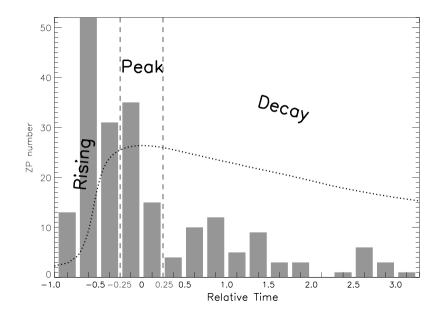
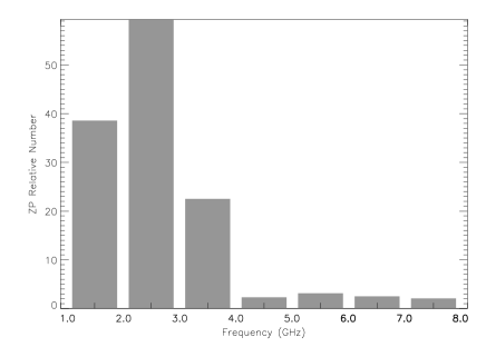
Figure 1: Left is the ZP distribution with respect to the phase time in flares. The dotted curve is an example profile of GOES soft X-ray emission in a typical flare. The two vertical dashed lines partition flaring process into rising, peak, and decay phases. Right is the ZP distribution with respect to the emission frequency.

(2) Polarization

Generally, the polarization sense of spectral fine structures is an important parameter. From Table 2, we may find that the microwave ZPs in a same flare may have almost all polarization modes from very weak (near 0) to very strong (near 100% at LCP or RCP). As there is no polarization observation from ORSC, here, we only analyze the polarization properties of the 154 ZPs obtained by SBRS/Huairou. Among these 154 ZP events, there are 68 (44.2%) ZPs have strong polarization degree ($r\geq 80\%$), 38 (24.7%) ZPs have moderate polarization degree ($20\%<r<80\%$), and 48 (31.1%) ZPs have no obviously polarizations ($r<20\%$). This fact indicates that there is no dominated polarization modes in microwave ZPs.

(3) Duration

Table 2 indicates that the duration of ZPs even in same flare are also distributed in a wide range from sub-second to several decades seconds. The left-lower panel of Figure 2 presents the distribution of ZP durations with respect to the relative time of ZP occurred in the flares, which shows that ZP duration has a moderate linear increase from the flare early rising phase to its late decay phase. The dash-dotted line is a result of chi-square goodness linear fitting. Although the distribution is very disperse in the flare rising and peak phases. Maybe the statistical averaged values of the ZP duration can give some supplementary inspirations. In the flare rising phase, the averaged ZP duration is 5.41 s with variance 8.85 s, and the relative variation is 1.64. Around the flare peak phase, the averaged ZP duration is 6.95 s with variance 11.03 s, and the relative variation is 1.59. While in the flare decay phase the averaged ZP duration is 17.55 s with variance 21.44 s, and the relative variation is 1.22, which is much smaller than that in the other two phases and in the whole sample.

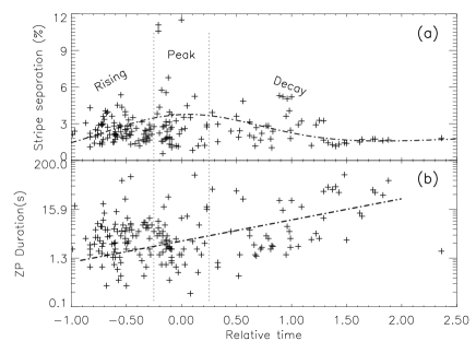
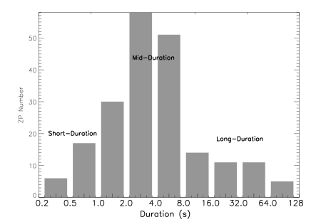
Figure 2: Left is the distributions of zebra stripe frequency separation (a) and durations (b) with respect to the phase time of ZP occurring. Right is the generalized ZP distribution with respect to the durations.

Actually, the minimum duration in the whole sample (with 202 ZP events) is only 0.2 s, while the longest duration is 95 s, which covers about 3 orders of magnitude. The right panel of Figure 2 presents a histogram of the distribution of ZPs numbers with respect to ZP durations. Here, we set the interval scale of the ZP duration in power exponent of 2. It is showed that there are 153 ZPs (75.7%) having the duration in range of 1 - 16 s, while only 23 ZPs (11.4%) have durations $<1.0$ s and 26 (12.9%) ZPs have durations $>16.0$ s. This fact implies that the very short and very long duration ZPs are very rare.

(4) Frequency separation of zebra stripes

The frequency separations between the adjacent zebra stripes are in the range of 14 - 340 MHz. It depends on the ZP central frequency. Generally, the higher ZP central frequency, the wider of the frequency separations among zebra stripes. We define a relative separation: $\Delta f/f_{zp}$, here, $\Delta f$ and $f_{zp}$ are the zebra stripe frequency separation and the ZP central frequency, respectively. The sixth and seventh column of Table 2 listed the $\Delta f$ and $\Delta f/f_{zp}$ in a typical flare, which indicates that $\Delta f/f_{zp}$ is in the range of several percents. In fact, among the whole sample, the maximum of $\Delta f/f_{zp}$ can be high up to 10%, while the minimum can be low down to below 1%. Statistical calculation indicates that averaged $\Delta f/f_{zp}$ is 2.42% in the flare rising phase, 3.23% in the flare peak phase, and 2.49% in the flare decay phase. This variation can be fitted by an exponential curve, showed in the left-bottom panel of Figure 2 (the dash-dotted curve), although it is very scattered in a broad range around the flare peak.

It is very interesting to investigate the variations of the frequency separation with respect to its frequency in each ZP event. In order to make such investigation, we just analyze the ZP events with at least 4 zebra stripes (there are at least 3 values of the frequency separation), and totally there are 151 ZP events occurring in 33 flares in our sample. Here, we find that there exist three kinds of obviously different variations of the frequency separation:

(1) Constant separation, the amplitude of $\triangle f$ variation does not exceed the frequency resolution of the spectrometer, which can be approximately regarded as a constant. A1 panel of Figure 3 is an example of this kind, here, the $\triangle f$ variation is 4 MHz, which is just the frequency resolution of the telescope.

(2) Varying separation, the amplitude of $\triangle f$ variation exceeds the frequency resolution of the spectrometer, and is scattered in a wide range. A2 panel of Figure 3 is an example of this kind, here, the total variation of $\triangle f$ is 44 MHz which is 11 times of the frequency resolution (4 Mhz) and has changes in addition-and-deletion.

(3) Rising separation, the amplitude of $\triangle f$ variation also exceeds the frequency resolution of the spectrometer and increases continuously with respect to its frequency. A3 panel of Figure 3 is an example of such kind.

4 Classification of ZPs

It is meaningful to make a physical classification of the microwave ZPs, which may help us to understand the basic properties of their origin and applications to solar eruptions. However, so far, there is no such work in the existing publications. The main reason is that it is very difficult to collect enough microwave ZP events to form a considerable big sample for a reasonable physical classification. The statistical analysis in above sections indicates that parameters of emission frequency, stripe frequency separation, polarization degree, stripe number, and the phase time in the associated flare are always distributed dispersively in wide ranges. For example, the ZPs occurred in flare rising phase may have all polarization degrees from very weak ($r\rightarrow 0$) to very strong ($r\rightarrow 100\%$) circular polarized modes as well as in flare peak phase or decay phase. The most of the other parameters also have the similar dispersive characteristics.

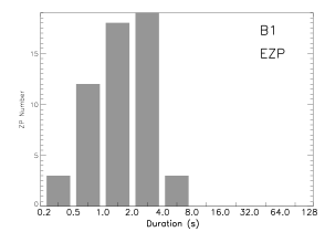
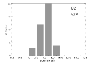
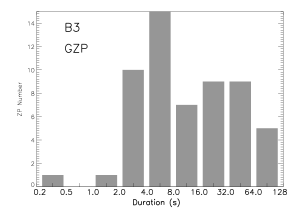
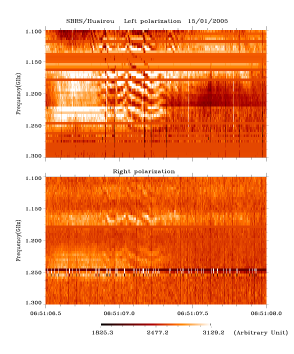
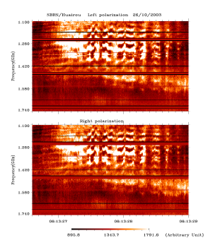
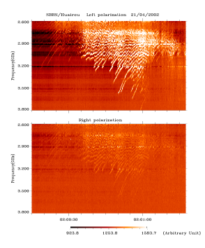
Figure 3: A1, A2, and A3 show the variations of the frequency separation between adjacent zebra stripes versus the stripe number from low to high frequency in typical equidistant ZP, variable-distant ZP, and growing-distant ZP; B1, B2, and B3 show the ZP distributions versus durations in these three ZP types; C1, C2, and C3 are the magnetic fields in the source regions deduced from each type of ZPs, respectively. The bottom panels are the spectrograms of typical equidistant ZP (left) with constant separation, variable-distant ZP (middle) with varying separation and growing-distant ZP (right) with rising separation, respectively.

However, the above analysis implies that it is very valuable when we combine duration and the variation of the frequency separation with respect to its frequency in each ZP event. According to these two factors, we may classify ZPs into three types with other parameters having relatively narrow range. The detailed properties can be presented as following:

Equidistant ZP (EZP), which stripe frequency separation approximates to a constant. Among the 151 ZPs with more than 4 stripes, there are 55 ZPs belonging to EZP, and their distribution to the duration is showed in B1 of Figure 3. Additionally, we find that (1) the durations of EZP is ranging from 0.3 s to 5.0 s, and most of them have durations around 1 - 2 s, the average duration is 1.6 s. (2) most EZPs are strong circular polarization, there are 33 short-duration ZPs observed by SBRS/Huairou which show that there are 20 events with strong circular polarizations, the averaged polarization degree $r\sim 70\%$. (3) most EZPs occurred in the flare rising and peak phases, only 7 events occurred at the flare decay phase, and the averaged $P_{ph}=-0.31$. (4) The zebra stripe number is less than 10 with average value of about 6.5. (5) Most EZPs are simple and isolated far away from the other spectral fine structures. The bottom left panel of Figure 3 is an example of EZP, which is very simple and isolated ZP without any other fine spectral structures before and after it. The duration is only 0.6 s, with strong left-handed circular polarization.

Variable-distant ZP (VZP), which stripe frequency separation varies in a wide range and with irregularly increasing or decreasing. Among the 151 ZPs, there are 39 ZPs belonging to VZP, and their distribution to the duration is showed in B2 of Figure 3. Additionally, we find that (1) the duration of VZP is in the range of 1.5 - 14 s, and most of them are around 2 - 10 s, the averaged value is 6.4 s. (2) The polarization degree has a very wide range from 0 to 100%. (3) VZPs can appear in flare rising, peak phases as well as in flare decay phase. (4) The zebra stripe number of VZP is also in a wide range of 2 - 28, and most of them are less than 10 stripes. (5) most VZPs are relatively complex, and always accompanying with other fine structures. The bottom middle panel of Figure 3 is a typical example of VZP, which is occurred in the rising phase of an X1.2 flare on 2003 October 26. The duration is 2.2 s with weakly polarization. It is a complex ZP modulated by a quasi-periodic pulsation with period of about 100 ms, similar to the quasi-periodic wiggles modulated by some MHD oscillations (Yu et al. 2013).

Growing-distant ZP (GZP), which stripe frequency separation has a big variation and increases continuously with respect to its frequency. Among the 151 ZPs, there are 57 ZPs belonging to GZPs, and their distribution to duration is showed in B3 of Figure 3. Additionally, we find that (1) their duration ranges from 0.2 s to 95 s, most of them are longer than 10 s, the average duration is 27.6 s. (2) most GZPs are moderate or very weak circular polarizations. Among these 57 GZPs, there are 35 events having polarization degree $r<50\%$. (3) most GZPs occurred in the flare decay phase. Totally, there are 41 ZPs occurring in flare decay phase, therein 25 ZPs belong to GZP. (4) most GZPs have more than 15 zebra stripes, the average stripe number in each ZP is 14.9, which is much more than that occurring in EZPs and VZPs. (5) most GZPs are very complex and accompanied or superimposed with many other spectral fine structures, such as fibers, spikes, narrow band type III bursts, fast quasi-periodic pulsations, etc. The bottom right panel of Figure 3 is a typical example of GZP, which is occurred in the very deep decay phase of a long-duration X1.5 flare on 2002 April 21. The ZP duration is about 70 s, besides its left-handed circular polarization can be distinguished bright zebra stripes, the right-handed circular polarization can be also identified zebra stripes clearly. It is a very complex ZP accompanying with many other spectral fine structures. On the whole, it is a combination of ZP structure with quasi-periodic wiggles at the relatively low frequency side and a fiber structure at the relatively high frequency side. On the details, each zebra stripe are consisting of superfine millisecond spikes (Chernov et al. 2005, Chen & Yan 2007).

Figure 3 can present a clearly comparison among the three kinds of ZP types. Actually, the comparison indicates that the above classification of microwave ZPs can present the different physical processes with each other to some extent, although there are a bit of overlapping between EZP and VZP, or between VZP and GZP at durations. Sometimes, there may be a transition from EZP to VZP, or from VZP to GZP in a same ZP structure.

As we know that BW model induced that the frequency separation between the adjacent zebra stripes is a constant and approximates the electron gyro-frequency $f_{ce}$, and all stripes may produce from a small compact source region. The corresponding duration will be very short, and the resulting spectrum has only a few harmonics (less than 10). These items conform with the basic characteristics of the EZPs. Therefore, BW model possibly reveals the basic mechanism of EZPs, and the stripe frequency separation can directly measure the magnetic field in the source region: $B\approx 3.56\times 10^{-7}\Delta f$. Here, the unit of $B$ is Gs, and $\Delta f$ in Hz. C1 panel of Figure 3 presents the magnetic fields in the source regions deduced from EZPs. Here, we find that the magnetic field strength ranges mainly from 10 Gs to 45 Gs, and has an increasing trend with emission frequencies.

DPR model proposes that zebra stripes is produced from some resonance levels where the upper hybrid frequency coincides with the harmonics of electron gyro-frequency in the inhomogeneous flux tube, and the frequency separation is dominated not only by the electron gyro-frequency, but also by the gradient of plasma density. Since the DPR levels present in the non-uniform trap and the kinetic instability can be excited by a small quantity of trapped non-equilibrium electrons, the DPR mechanism can provide a fairly large number of stripes (e.g., more than 20 stripes) in the ZP spectra with comparatively long durations. Based on the common value of magnetic field and plasma density around the flaring source region, we know that the frequency separation will have a slowly increase with respect to the frequency. These facts conform with the main characteristics of GZPs, which shows that DPR model may explain their formation. By using DPR model, we can also deduce the magnetic fields in the source region: $B\approx 3.56\times 10^{-7}Q\cdot\Delta f$, $Q=\frac{1}{n}|\frac{2H_{p}}{H_{b}}-1|$, when polarization is strong, $n=1$, and when polarization is weak, $n=2$. C3 panel of Figure 3 is the distribution of magnetic field strength with respect to emission frequency deduced from GZPs, the magnetic field strength ranges from 10 Gs to 75 Gs, which is more dispersed than that of EZPs and VZPs.

It seems very difficult to make a reasonable explanation to the formation of VZPs for their irregular variation of frequency separations. WW model induced that the zebra stripes frequency separation is about: $\Delta f=2f_{w}$, and the whistler wave frequency: $f_{w}\approx 0.1-0.5f_{ce}$, here, $f_{ce}\ll f_{pe}$. Therefore, $\Delta f$ will have variations in a relatively narrow band. These properties seem to indicate that the WW model should be the possible mechanism to explain the formation of VZPs. Applying WW model, an approximated estimation of the magnetic field in the source region can be obtained. As we know that the whistler wave group velocity peaks at frequency $\frac{1}{4}f_{ce}$, which indicates that the frequency separation $\Delta f$ may vary around $\frac{1}{2}f_{ce}$. Then we may estimate the magnetic field strength just by the frequency at whistler peak group velocity: $B\approx 7.12\times 10^{-7}\Delta f$. C2 panel of Figure 3 is the distribution of magnetic field strength with respect to emission frequency deduced from VZPs by above method. Here, we find that the magnetic field strength ranges from 10 Gs to 145 Gs, which is stronger and much wider distribution than that in the source of EZPs. However, as we know that the WW model has many problems which have not been proved so far. There are many work need to study comprehensively. The diversity of polarization sense of VZPs imply that it is also possible that the VZP may be a blended spectral structure produced from some combined mechanisms (for example, the propagating model, or the combination of DPR and WW models, etc.).

Because the BW mechanism requires a larger number of non-equilibrium electrons than that of DPR mechanism, and there are more non-equilibrium electrons in the flare rising phase for the continuously magnetic reconnection than that in the flare decay phase, BW mechanism may be more preferential to work in the flare early phase and small source region to produce EZPs. The DPR mechanism may be more preferential to work in the flare decay phase and produce GZPs from different resonance levels in relatively stable flaring loop. In the flare decay phase, there are many small scale magnetic reconnections and energy releases in the hot magnetized plasma loops, many small scale microwave bursts (Tan 2013) may take place accompanying with microwave ZPs, such as microwave spikes, narrow band type III bursts, and fast quasi-periodic pulsations or wiggles (Tan et al. 2007, Yu et al. 2013). In WW mechanism, the low-frequency whistler waves are excited by non-equilibrium electrons with loss-cone distributions in coronal traps with intermittent non-uniform layers (Chernov 2006), such conditions may appear in all phases of solar flares, and therefore VZPs may take place in all flaring phases.

5 Conclusions and Discussions

There are many parameters which apply to describe the characteristics of microwave ZPs associated with solar flares, such as the central frequency ($f_{zp}$), phase time ($P_{ph}$), polarization degree ($r$), zebra stripe number ($N_{str}$), duration ($D_{zp}$), frequency separation between adjacent zebra stripes ($\Delta f$) and the relative value ($\Delta f/f$). However, from the statistical investigation, we find that most parameters can not act as the classifying indicator of microwave ZPs, while the combination of duration and the variation of the frequency separation with respect to its frequency in each ZP event may provide a physical classification. With such combination, we may classify the microwave ZPs into three types:

(1) EZP, simple and isolated with constant frequency separation of the adjacent zebra stripes, very short duration ($1.0-2.0s$), relatively strong polarization, less than 10 stripes, and mainly occurred in the flare rising phase.

(2) VZP, relatively complex with irregular varying frequency separation of the adjacent zebra stripes and mid-term durations ($2.0-10.0s$), diverse polarization modes, and always overlapped by some other structures, such as quasi-periodic pulsations or wiggles, etc.

(3) GZP, very complex with increasing frequency separation of the adjacent zebra stripes and long duration ($>10s$), relatively weak polarization, and mainly occurred in the flare decay phase with more than 10 stripes and accompanying with many spectral fine structures, such as spikes, fibers, and quasi-periodic pulsations.

Different types of microwave ZPs may have different formation mechanisms, and therefore may reveal different physical processes in the source regions. The main properties of EZP indicate that the BW model should be the best mechanism to explain its formation. VZPs may produce from WW wave mechanism or from some complex multi-mechanisms. And the DPR model may reveal the physical processes of GZPs. The estimation of the magnetic field strengths deduced from the above models and ZP structures shows that the magnetic field in the microwave ZP source regions ranges from 10 Gs to 145 Gs, which is in the acceptable domain of the magnetic field in coronal flaring source regions.

The above classification may help us to clarify the controversies among the existing various ZP models. Of course, since the theories of BW model, WW model, and DPR model are far from perfect (Zlotnik 2009). Many physical details are still not clear, we do not know exactly which model is the best one to explain the formation of a given ZP event. For example, it is difficult to distinguish whether a ZP with only three or less zebra stripes belongs to EZP, or VZP, even or GZP. We have to look for other properties of ZPs and further theoretical and observational investigations. The another problem is the formation of VZPs for their diversity and irregularity, it is possible that it is formed from some complex mechanism. Additionally, it is still a big problem why some zebra stripes are composed of many millisecond spikes with super-high brightness temperature? And what is the physical relationship between ZP structure and its inner millisecond spikes? These questions need us to study more comprehensively, especially the observational information with high spatial resolutions at the corresponding frequencies.

From the statistical analysis, it is found that microwave ZPs can occur in the flare rising and peak phases as well as in the flare decay phase, especially more preferential to produce in long-duration powerful flares around frequency of 3.00 GHz. Such fact implies that there are some common characters attached in microwave ZPs. As we know the microwave emission source region around 3.00 GHz is possibly very closed to the core region of solar flaring and energy releasing, microwave ZPs may reveal some fundamental nature of solar eruptive processes.

References

- Barta (2006) Bárta, M., & Karlický, M., 2006, AA, 450, 359
- Berney (1978) Berney, M., & Benz, A.O., 1978, AA, 65, 369
- Chen (2007) Chen, B., & Yan, Y.H., 2007, Solar Phys., 246, 431
- Chernov (1976) Chernov, G.P., 1976, Sov. Astron., 20, 582
- Chernov (1990) Chernov, G.P., 1990, Solar Phys., 130, 75
- Chernov (2005) Chernov, G.P., Yan, Y.H., Fu, Q.J., & Tan, C.M., 2005, AA, 437, 1047
- Chernov (2006) Chernov, G.P., 2006, Space Sci. Rev., 127, 195
- Chiuderi (1973) Chiuderi, C., Giaghetti, R., & Rosenberg, H., 1973, Solar Phys., 33, 335
- Fu (1995) Fu, Q.J., Qin, Z.H., Ji, H.R., & Pei, L., 1995, Sol. Phys., 160, 97
- Fu (2004) Fu, Q.J., Ji, H.R., Qin, Z.H. et al., 2004, Sol. Phys., 222, 167
- Huang (2008) Huang, J., Yan, Y.H., Liu, Y.Y., 2008, Sol. Phys., 253, 143
- Huang (2010) Huang, J., Yan, Y.H., Liu, Y.Y., 2010, Adv. Space Res., 46, 1388
- Huang (2012) Huang, J., Tan, B.L., 2012, ApJ, 745, 186
- Jiricka (1993) Jirícká, K., Karlický, M., Kepka, O., & Tlamicha, A., 1993, Sol. Phys., 147, 203
- Karlicky (2013) Karlický, M., 2013, AA, 552, 90
- Kuijpers (1975) Kuijpers, J., 1975, Sol. Phys., 44, 173
- Kuznetsov (2005) Kuznetsov, A.A., 2005, AA, 438, 341
- Kuznetsov (2007) Kuznetsov, A.A., & Tsap, Yu, 2007, Solar Phys., 241, 127
- LaBelle (2003) LaBelle, J., Treumann, R. A., Yoon, P.H., & Karlichy, 2003, ApJ,593, 1195
- Ledenev (2006) Ledenev, V.G., Yan, Y.H., & Fu, Q.J, 2006, Solar Phys., 233, 129
- Maltseva (1989) Maltseva, O.A., & Chernov, G.P., 1989, KFNT, 5, 44
- Pearlstein (1966) Pearlstein, L.D., Rosenbluth, M.N., & Chang, D.B., 1966, Phys. Fluid, 9, 953
- Rosenberg (1972) Rosenberg, H., 1972, Solar Phys., 25, 188
- Tan (2007) Tan, B.L., Yan, Y.H., Tan, C.M., & Liu, Y.Y., 2007, ApJ, 671, 964
- Tan (2010) Tan, B.L., 2010, Astrophys. Space Sci., 325, 251
- Tan (2013) Tan, B.L., 2013, ApJ, 773, 165
- Winglee (1986) Winglee, R.M., & Dulk, G.A., 1986, ApJ, 307, 808
- Yan et al (2002) Yan, Y.H., Tan, C.M., & Xu, L., et al., 2002, Sci. Chin. A Suppl., 45, 89.
- Yasnov (2004) Yasnov, L., & Karlicky, M.G., 2004, Sol. Phys., 219, 289
- Yu (2012) Yu, S.J., Yan, Y.H., & Tan, B.L.: 2012, ApJ, 761, 136
- Yu (2013) Yu, S.J., Nakariakov, V.M., Seilzer, L.A., Tan, B.L., & Yan, Y.H.: 2013, ApJ, 777, 159
- Zaitsev (1983) Zaitsev, V. V. & Stepanov, A. V., 1983, Sol. Phys., 88, 297
- Zheleznyakov (1975) Zheleznyakov, V.V., & Zlotnik, E.YA, 1975, Solar Phys., 44, 461
- Zlotnik (2003) Zlotnik, E. Ya, Zaitsev, V.V., Aurass, H., Mann, G., & Hofmann, A., 2003, AA, 410, 1011
- Zlotnik (2009) Zlotnik, E. Ya, 2009, Cent. Eur. Astrophys. Bull., 33, 281