Three-body bound states in dipole-dipole interacting Rydberg atoms

Abstract

We show that the dipole-dipole interaction between three identical Rydberg atoms can give rise to bound trimer states. The microscopic origin of these states is fundamentally different from Efimov physics. Two stable trimer configurations exist where the atoms form the vertices of an equilateral triangle in a plane perpendicular to a static electric field. The triangle edge length typically exceeds $R\approx 2\,\mu\text{m}$, and each configuration is two-fold degenerate due to Kramers’ degeneracy. The depth of the potential wells and the triangle edge length can be controlled by external parameters. We establish the Borromean nature of the trimer states, analyze the quantum dynamics in the potential wells and describe methods for their production and detection.

Rydberg atoms gallagher:ryd are ideal candidates for the investigation of few-body quantum phenomena for several reasons. First, their internal and external degrees of freedom can be accurately controlled and manipulated in state-of-the-art experiments. This gives rise to theoretically well-understood and tunable dipole-dipole (DD) interactions saffman:10 ; beguin:13 between ultra-cold Rydberg atoms. Second, the range of these DD interactions is extremely large - it typically extends to several microns. This feature allows the study of few-body quantum systems whose constituents can be prepared, manipulated and detected individually. Several quantum phenomena arising from strong interactions between two Rydberg atoms were investigated recently. Examples are given by the Rydberg blockade effect jaksch:00 ; lukin:01 ; urban:09 ; gaetan:09 and the realization of quantum gates and entanglement wilk:10 ; isenhower:10 . Rydberg atoms can form giant diatomic molecules via different binding mechanisms between their constituents greene:00 ; bendkowsky:09 ; boisseau:02 ; samboy:11 ; kiffner:12 ; overstreet:09 . Artificial gauge fields induced by the DD interaction yao:12 ; yao:13 and acting on the relative motion of two Rydberg atoms were predicted in zygelman:12 ; kiffner:13 ; kiffner:13b .

In few body-physics, systems with three particles often show qualitatively different features as compared to two particles pohl:09 ; wuster:11 ; yarkony:96 ; domcke:ci ; efimov:70 ; kraemer:06 ; pollack:09 ; roy:13 ; braaten:06 ; wang:11 ; efremov:13 . For example, it has been shown pohl:09 that the dipole blockade can be broken by adding a third Rydberg atom. Furthermore, it has been predicted wuster:11 that systems of more than two DD interacting atoms exhibit conical intersections yarkony:96 ; domcke:ci , which are relevant for photo-chemical processes. A paradigm of few-body quantum physics is the Efimov effect efimov:70 ; kraemer:06 ; pollack:09 ; roy:13 . Here a short-range resonant two-body interaction between identical bosons gives rise to a universal set of bound trimer states braaten:06 . Recently, it was shown that the Efimov effect persists wang:11 even for a resonant long-range DD interaction.

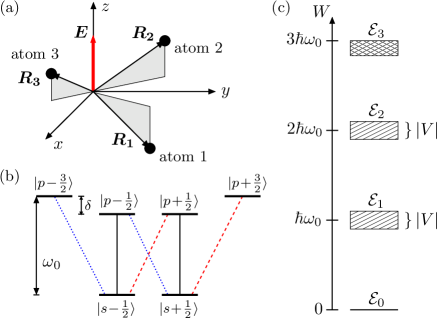
Figure 1: (Color online) (a) System configuration of three DD interacting Rydberg atoms. $\boldsymbol{R}_{\alpha}$ is the position of atom $\alpha$. An external electric field $\boldsymbol{E}$ is applied in the $z$ direction. (b) Internal level structure of each Rydberg atom. The Stark shifts $\hbar\delta\equiv W_{p\pm 1/2}-W_{p\pm 3/2}$ of the $|p\pm 1/2\rangle$ states are negative and $\omega_{0}$ is the transition frequency on the $|p\pm 3/2\rangle\leftrightarrow|s\pm 1/2\rangle$ transitions kiffner:12 . The dipole transitions indicated by solid, blue dotted and red dashed lines couple to $\pi$, $\sigma^{-}$ and $\sigma^{+}$ polarized fields, respectively. (c) Level structure of the three-atom state space. $\mathcal{E}_{i}$ contains all states where $i$ atoms are in an $np$ state and all other in an $ns$ state. States within $\mathcal{E}_{1}$ and $\mathcal{E}_{2}$ are coupled by the DD interaction $V$.

Here we show that the DD interaction between three distant Rydberg atoms with non-overlapping electron clouds can induce bound trimer states. These states arise from the rich internal level structure of the Rydberg atoms. A crucial point is the presence of several dipole transitions in each atom and the interplay between distance-dependent DD interactions and Stark-shifted Zeeman states. In stark contrast to the systems described in efimov:70 ; kraemer:06 ; pollack:09 ; wang:11 , the two-body interaction in our setup cannot be described by a single scattering length exceeding all physically relevant length scales. The microscopic origin of our states is thus fundamentally different from universal Efimov states. The considered setup is shown in Fig. 1, and the level scheme of each atom was introduced in the context of Rydberg macrodimers kiffner:12 . We find two stable trimer configurations where the atoms form the vertices of an equilateral triangle in a plane perpendicular to a static electric field [see Fig. 2(a)]. The triangle edge length typically exceeds $R\approx 2\,\mu\text{m}$ and thus the bound states occur at extremely long range which is experimentally resolvable. We find that our Hamiltonian gives rise to Kramers’ degeneracy, and thus the two trimer potential curves are two-fold degenerate. The depth of the potential well and the triangle edge length can be controlled by the external electric field and the principal quantum number of the Rydberg level. We discuss the width and the depth of the potential wells and describe methods for their production and detection. The stable trimer configurations arise from a genuine three-particle effect since two-atom systems are unbound for the considered atomic setup. The nature of the trimer bond can thus be illustrated by the Borromean rings shown in Fig. 2(b): If any of the three rings is removed, the remaining two are unbound.

The geometry of the three-atom system is shown in Fig. 1(a). We denote the position of atom $\alpha$ by $\boldsymbol{R}_{\alpha}$, and a DC electric field $\boldsymbol{E}$ in the $z$ direction defines the quantization axis. The Born-Oppenheimer potential surfaces of this system are determined by the Hamiltonian

$$H=\sum\limits_{\alpha=1}^{3}H_{\text{A}}^{(\alpha)}+V_{13}+V_{23}+V_{12},$$ (1)

where $H_{\text{A}}^{(\alpha)}$ describes the internal levels of atom $\alpha$ kiffner:12 . In each Rydberg atom we consider two angular momentum multiplets as shown in Fig. 1(b). The lower $ns_{1/2}$ states have total angular momentum $J=1/2$, and the excited multiplet is comprised of $np_{3/2}$ states with total angular momentum $J=3/2$. We specify the individual atomic states $|\ell m_{j}\rangle$ by their orbital angular momentum $\ell$ and azimuthal total angular momentum $m_{j}$. The energy difference $\hbar\delta\equiv W_{p\pm 1/2}-W_{p\pm 3/2}$ denotes the Stark shift of the $|p\pm 1/2\rangle$ states with respect to the $|p\pm 3/2\rangle$ states. The symbol $V_{\alpha\beta}$ in Eq. (1) represents the DD interaction tannoudji:api between atoms $\alpha$ and $\beta$,

$$V_{\alpha\beta}=\frac{1}{4\pi\varepsilon_{0}R_{\alpha\beta}^{3}}[\boldsymbol{\hat{d}}^{(\alpha)}\cdot\boldsymbol{\hat{d}}^{(\beta)}-3(\boldsymbol{\hat{d}}^{(\alpha)}\cdot\vec{\boldsymbol{R}}_{\alpha\beta})(\boldsymbol{\hat{d}}^{(\beta)}\cdot\vec{\boldsymbol{R}}_{\alpha\beta})],$$ (2)

where $\boldsymbol{\hat{d}}^{(\alpha)}$ is the electric dipole-moment operator of atom $\alpha$, $\boldsymbol{R}_{\alpha\beta}=R_{\alpha}-R_{\beta}$ describes the relative position of atom $\alpha$ with respect to atom $\beta$ and $\vec{\boldsymbol{R}}_{\alpha\beta}=\boldsymbol{R}_{\alpha\beta}/R_{\alpha\beta}$ is the corresponding unit vector.

The total state space $\mathcal{E}$ of the three atoms is spanned by the $6^{3}=216$ tensor product states of the individual atoms, $|\ell m_{j}\rangle\otimes|\tilde{\ell}\tilde{m}_{j}\rangle\otimes|\ell^{\prime}m^{\prime}_{j}\rangle$. We divide $\mathcal{E}$ into four subspaces $\mathcal{E}_{i}$ ($i\in\{0,1,2,3\}$), where $\mathcal{E}_{i}$ contains all three-atom states with $i$ atoms in an $np$ state and $3-i$ atoms in an $ns$ state. All three-atom states belonging to different subspaces are well separated in energy. This is shown in Fig. 1(c), illustrating that states in $\mathcal{E}_{i}$ are clustered around $i\times\hbar\omega_{0}$. Due to the large energy separation of the subspaces $\mathcal{E}_{i}$ we neglect any DD induced coupling between them and diagonalize $H$ in Eq. (1) in each subspace independently. The DD interaction $V$ in Eq. (2) vanishes in $\mathcal{E}_{0}$ and $\mathcal{E}_{3}$. On the contrary, $V$ has non-zero matrix elements between the $N_{1}=48$ ($N_{2}=96$) states in $\mathcal{E}_{1}$ ($\mathcal{E}_{2}$). Since the bare three-atom states in $\mathcal{E}_{1}$ ($\mathcal{E}_{2}$) differ at most by $\hbar|\delta|$ ($2\hbar|\delta|$) in energy, they are coupled resonantly by the DD interaction $V\propto 1/R^{3}$ for interatomic distances $R\leq R_{0}$. The characteristic length scale $R_{0}$ where the strength of the DD interaction equals $\hbar|\delta|$ is

$$R_{0}=[|\mathcal{D}|^{2}/(4\pi\epsilon_{0}\hbar|\delta|)]^{1/3},$$ (3)

and $|\mathcal{D}|$ is the reduced dipole matrix element of the $ns\leftrightarrow np$ transition kiffner:12 . The value of $R_{0}$ can be adjusted via the principal quantum number $n$ of the Rydberg level and the DC electric field and is typically of the order of several microns (see below).

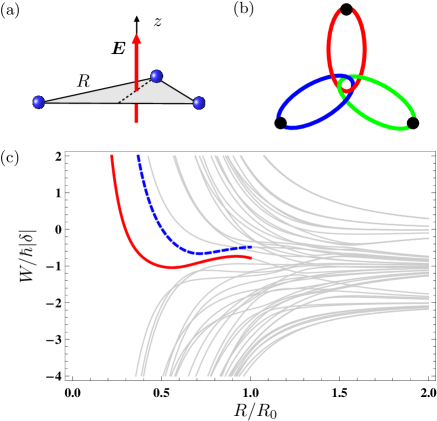
Figure 2: (Color online) (a) Geometry where the atoms form the vertices of an equilateral triangle with edge length $R$ in the $x-y$ plane. The $z$ direction is distinguished by an external electric field $\boldsymbol{E}$. (b) illustrates the Borromean nature of the trimer configurations. (c) All potential curves within the manifold $\mathcal{E}_{2}$. The solid red curve shows $\epsilon_{\text{t}}$, and the blue dashed curve labels $\epsilon_{\text{s}}$. $W+2\hbar\omega_{0}$ represents the absolute energies of the potential curves.

The Hamiltonian in Eq. (1) is time-reversal invariant haake:qsc ; supp . The time-reversal operator is given by $T=\exp(\imath\pi J_{y})\mathcal{K}$, where $J_{y}$ is the $y$ component of the spin angular momentum operator of the three atoms and $\mathcal{K}$ denotes complex conjugation with respect to the basis states $|\ell m_{j}\rangle\otimes|\tilde{\ell}\tilde{m}_{j}\rangle\otimes|\ell^{\prime}m^{\prime}_{j}\rangle$. Since $T^{2}=-1$, the time-reversal symmetry gives rise to Kramers’ degeneracy; every eigenvalue of $H$ in Eq. (1) is (at least) two-fold degenerate.

The main result of this letter is that our system exhibits two stable trimer configurations if the atoms form the vertices of an equilateral triangle in the $x-y$ plane [see Fig. 2(a)]. A first indication for three-body bound states is shown in Fig. 2(c), where all potential curves in the $\mathcal{E}_{2}$ manifold are shown as a function of the triangle edge length $R$. We refer to the potential curve represented by the red solid (blue dashed) line as $\epsilon_{\text{t}}$ ($\epsilon_{\text{s}}$). The latter two potential curves exhibit a clear minimum, and are well isolated from all other curves. Each potential curve is two-fold degenerate due to Kramers’ degeneracy, thus giving rise to four trimer states. The minima in $\epsilon_{\text{t}}$ and $\epsilon_{\text{s}}$ can be explained with the same mechanism leading to bound dimer states kiffner:12 . As the separation between atom pairs is reduced, the DD interaction becomes stronger and eventually couples non-degenerate three-atom states. These couplings lead to avoided crossings between repulsive and attractive potential curves and to the formation of potential wells.

In order to establish that the minima shown in Fig. 2(c) correspond to bound three-particle states, we describe the spatial degrees of freedom in terms of the centre-of-mass coordinate and two relative position vectors $R_{\alpha 3}$ ($\alpha\in\{1,2\}$) supp ,

$$\boldsymbol{R}_{\alpha 3}=R_{\alpha 3}(\sin\theta_{\alpha}\cos\phi_{\alpha},\sin\theta_{\alpha}\sin\phi_{\alpha},\cos\theta_{\alpha}).$$ (4)

Since the DD interaction in Eq. (2) depends only on $R_{13}$ and $R_{23}$, the energy surfaces do not depend on the centre-of-mass coordinates. In addition, the energies are independent of the sum $\phi_{1}+\phi_{2}$ due to the azimuthal symmetry of the system. We set $\phi_{1}+\phi_{2}=0$ such that we have $\phi_{1}=\phi/2$ and $\phi_{2}=-\phi/2$, where $\phi=\phi_{1}-\phi_{2}$. It follows that all eigenvalues of the Hamiltonian in Eq. (1) are uniquely described in terms of five independent variables $\boldsymbol{v}=(R_{13},R_{23},\theta_{1},\theta_{2},\phi)$.

The potential well $\epsilon_{\text{t}}$ in Fig. 2(c) has a local minimum as a function of the triangle edge length $R$ at $R_{\text{t}}=0.56R_{0}$. This minimum corresponds to the parameters $\boldsymbol{v}_{\text{t}}=(R_{\text{t}},R_{\text{t}},\pi/2,\pi/2,\pi/3)$. We evaluate the gradient and the Hessian matrix of $\epsilon_{\text{t}}$ with respect to the independent variables $\boldsymbol{v}$ and find supp that $\epsilon_{\text{t}}$ has indeed a local minimum at $\boldsymbol{v}_{\text{t}}$. For practical purposes it is important to know how deep and how broad the potential minima are around their equilibrium positions. The energy surface $\epsilon_{\text{t}}$ is shown in Fig. 3(a) as a function of $R_{13}$ and $R_{23}$ for $\theta_{1}=\theta_{2}=\pi/2$ and $\phi=\pi/3$. On the other hand, Fig. 3(b) shows the dependence of $\epsilon_{\text{t}}$ on $\theta_{1}$ and $\theta_{2}$ for $R_{13}=R_{23}=R_{\text{t}}$ and $\phi=\pi/3$. The width of this potential well about $\theta_{1}=\theta_{2}=\pi/2$ is approximately $\pm 45^{\circ}$. These results demonstrate that the potential curve $\epsilon_{\text{t}}$ exhibits a relatively broad minimum with respect to all variables. Similarly, we find supp that $\epsilon_{\text{s}}$ has a local minimum for $\boldsymbol{v}_{\text{s}}=(R_{\text{s}},R_{\text{s}},\pi/2,\pi/2,\pi/3)$ with $R_{\text{s}}=0.71\,R_{0}$. The minimum of the potential curve $\epsilon_{\text{s}}$ is more shallow and narrower as compared to $\epsilon_{\text{t}}$ [see Figs. 3(c) and (d)]. The minimal depth of the potential well in $\epsilon_{\text{t}}$ ($\epsilon_{\text{s}}$) is $0.3\,\hbar|\delta|$ ($0.14\,\hbar|\delta|$).

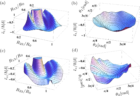
Figure 3: (Color online) (a) Variation of the shifted energy surface $\tilde{\epsilon}_{\text{t}}=\epsilon_{\text{t}}-2\hbar\omega_{0}$ with $R_{13}$ and $R_{23}$ for $\theta_{1}=\theta_{2}=\pi/2$ and $\phi=\pi/3$. (b) Dependence of $\tilde{\epsilon}_{\text{t}}$ on $\theta_{1}$ and $\theta_{2}$ for $R_{13}=R_{23}=R_{\text{min}}$ and $\phi=\pi/3$. (c) and (d) correspond to (a) and (b), respectively, with $\tilde{\epsilon}_{\text{t}}$ replaced by $\tilde{\epsilon}_{\text{s}}=\epsilon_{\text{s}}-2\hbar\omega_{0}$.

We emphasize that the bound trimer states arise from a genuine three-particle effect, i.e., they cannot be explained by a pairwise binding of the atoms. In order to establish this result, we consider any of the trimer states at the local minimum of the corresponding potential curve and calculate the reduced quantum state $\rho_{\text{dimer}}$ of two atoms. Since all trimer states are entangled, $\rho_{\text{dimer}}$ is a mixed state. We find that $1/3$ of the population of $\rho_{\text{dimer}}$ resides in the $npnp$ subspace which experiences no first-order DD interaction. The remaining $2/3$ of the population is found in $nsnp$ states that are DD coupled. However, all two-atom potential curves are either strongly repulsive or attractive for interatomic separations $R_{\text{t}}$ or $R_{\text{s}}$ kiffner:12 ; supp , leading to attraction and subsequent ionization or repulsion on timescales much shorter than the Rydberg lifetime li:05 ; amthor:07 ; viteau:08 ; park:11b . It follows that the pairwise interaction cannot explain the stability of the trimer configurations which establishes the Borromean nature of the three-particle bound states.

Next we study the quantum dynamics of the atoms in the trimer configuration by a harmonic approximation of the potential well $\epsilon_{\text{t}}$ near its local minimum supp . Since the momenta corresponding to the relative coordinates $\boldsymbol{R}_{13}$ and $\boldsymbol{R}_{23}$ are coupled in the kinetic energy part of the Hamiltonian, the normal modes are not simply given by the eigenvalues and eigenvectors of the Hessian matrix with respect to the relative coordinates. We find that the normal mode with the largest frequency $\omega_{\text{s}}=2.93\sqrt{\hbar|\delta|/(\mu R_{0}^{2}})$ is the symmetric stretch mode. There are five different eigenmodes in total, and all frequencies are of the same order of magnitude. The scissor and asymmetric stretch modes describe oscillations in the $x-y$ plane and are degenerate. The remaining two modes (wagging and twisting) are degenerate as well and correspond to oscillations in the $z$ direction.

The depth and the spatial extend of the trimer potentials near their local minima can be adjusted by the strength of the DC electric field and the principal quantum number $n$ of the Rydberg excitation. The DC electric field is typically of the order of $1\,V/\text{cm}$ anderson:98 and determines the Stark splitting directly, and $\hbar\delta$ and $n$ determine the characteristic length scale $R_{0}$ in Eq. (3). We note that $\hbar\delta$ and $n$ cannot be chosen independently. In particular, the Stark splitting of the $np_{3/2}$ level must be small compared to the $np$ fine structure interval $E_{\text{FS}}$. In order to give an explicit example, we consider Rb or Cs where $E_{\text{FS}}\sim 0.01n^{-3}E_{\text{h}}$ gallagher:ryd and $R_{0}=[E_{\text{h}}n^{4}/(3|\hbar\delta|)]^{1/3}a_{0}$ kiffner:12 . Here $E_{\text{h}}$ is the Hartree energy and $a_{0}$ the Bohr radius. A reasonable constraint on $\delta$ is thus given by $\hbar|\delta|<1.5\times 10^{-4}n^{-3}E_{\text{h}}$. Note that this choice implies $R_{0}>(10^{4}n/4.5)^{1/3}n^{2}a_{0}$, ensuring that $R_{0}$ is substantially larger than an individual Rydberg atom. For Rb $n=40$ atoms with $\delta=2\pi\times 10$ MHz we find $R_{0}=4.37\,\mu\text{m}$, $R_{\text{t}}=2.45\,\mu\text{m}$ and $R_{\text{s}}=3.12\,\mu\text{m}$. These parameters result in $\omega_{\text{s}}/(2\pi)\approx 33\,\text{kHz}$ for the largest oscillation frequency in the potential well $\epsilon_{\text{t}}$. The lifetime of the trimer states can be calculated from the 300 K radiative lifetimes of the $ns$ and $np$ Rydberg states beterov:09 . We find that the lifetime of the trimer state $|\psi_{\text{t}}\rangle$ is given by $45.5\,\mu\text{s}$ for $n=40$, resulting in roughly $1.5$ oscillations in the well before the atoms decay. We emphasize that this number can be increased for smaller principal quantum numbers $n$. For example, for Rb $n=30$ atoms with $\delta=2\pi\times 36$ MHz, the atoms oscillate 3 times during the lifetime and hence these oscillations can in principle be resolved via spectroscopic techniques.

The experimental implementation of our scheme can be realized in different ways. Optical potentials allow one to prepare three ground state atoms in the triangle configuration with the equilibrium edge length $R_{\text{t}}$ or $R_{\text{s}}$. For example, this could be achieved with an optical tweezer setup similar to the one described in gaetan:09 ; urban:09 . Alternatively, one could utilize Kagomé optical lattices santos:04 or engineer the desired triangular structure via the controlled occupation of specific sites in, e.g., a triangular lattice via advanced experimental techniques Weitenberg2011 . Subsequently all three atoms are excited in a two-photon process to the $ns$ Rydberg level park:11 ; park:11b ; miroshnychenko:10 ; li:05 . These states experience only a weak van der Waals shift such that the dipole blockade effect is negligible. The desired trimer state can then be excited by microwave radiation. Since states in the subspace $\mathcal{E}_{2}$ have no direct dipole matrix element with the $ns$ states in $\mathcal{E}_{0}$, the trimer states have to be excited via a two-photon process. We find that the trimer states have large dipole matrix elements with states in $\mathcal{E}_{1}$, and thus efficient excitation processes are possible via tailored microwave fields. From recent experiments miroshnychenko:10 ; park:11 we estimate that the two-step excitation can be achieved in less than $1\,\mu\text{s}$. Since ultra-cold Rydberg atoms are effectively stationary on this timescale, the atoms remain in their initial configuration during the excitation process.

A necessary condition for the detection of the trimer states is that their kinetic energy is smaller than the depth of the local minima in $\epsilon_{\text{t}}$ and $\epsilon_{\text{s}}$. The minimal depth for the potential curve $\epsilon_{\text{t}}$ ($\epsilon_{\text{s}}$) and for the $n=40$ Rubidium parameters above corresponds to a temperature of $144\,\mu\text{K}$ ($67\,\mu\text{K}$). This is much higher than typical temperatures of atoms in optical lattices, and still higher than the temperature of laser-cooled atoms in optical tweezers tuchendler:08 . There are several routes towards the detection of atoms in stable trimer configurations. First, they can be detected by spectroscopic methods similar to the suggested procedure for the detection of dimer states in kiffner:12 . Here the microwave excitation from a trimer state to another state showing no DD interaction should exhibit a resonant feature removed from the atomic transition by the well depth. Second, advanced imaging techniques schwarzkopf:11 ; schauss:12 allow one to observe spatially resolved patterns of Rydberg excitations. While Rydberg atoms in attractive or repulsive three-atom states will quickly leave their initial spatial configuration li:05 ; amthor:07 ; viteau:08 ; park:11b , stable trimer configurations will stay put. Thus the direct observation of the triangular configuration of Rydberg atoms after a time delay following their excitation would provide further evidence for the preparation of a trimer state. In conclusion, we are confident that the trimer states can be produced and detected with current experimental techniques.

In summary, we have shown that three dipole-dipole interacting Rydberg atoms can give rise to bound trimer states. Our scheme applies to ultra-cold Rydberg atoms where experimental techniques offer exquisite control over the external and internal atomic degrees of freedom. The trimer states are well separated from other potential curves such that the quantum dynamics remains adiabatic. Finally, we would like to mention that the opposite regime of non-adiabatic spin dynamics, whose study is beyond the scope of this work, might also give rise to novel few body effects. For instance, we find that the spectrum of the system Hamiltonian exhibits level repulsion haake:qsc , and hence expect the atomic motion to display chaotic behavior in the semi-classical regime. Moreover, in the absence of geometrical symmetries our time-reversal invariant Hamiltonian belongs to the symplectic symmetry class, giving rise to as yet unobserved quartic level repulsion haake:qsc . In conclusion, our system offers fascinating possibilities for future theoretical and experimental studies with ultra-cold and semi-classical Rydberg atoms.

I Time-reversal symmetry

The action of the time-reversal operator $T=\exp(\imath\pi J_{y})\mathcal{K}$ on the three-atom states $|\ell m_{j}\rangle\otimes|\tilde{\ell}\tilde{m}_{j}\rangle\otimes|\ell^{\prime}m^{\prime}_{j}\rangle$ changes the sign of the magnetic quantum number in each state,

$$T|\ell m_{j}\rangle\otimes|\tilde{\ell}\tilde{m}_{j}\rangle\otimes|\ell^{\prime}m^{\prime}_{j}\rangle$$

$$=\pm|\ell-m_{j}\rangle\otimes|\tilde{\ell}-\tilde{m}_{j}\rangle\otimes|\ell^{\prime}-m^{\prime}_{j}\rangle.$$ (5)

Since the atomic level scheme in Fig. 1(a) of the manuscript is symmetric with respect to a sign change of the magnetic quantum number, $T$ commutes with the atomic Hamiltonian,

$$\left[T,\sum\limits_{\alpha=1}^{3}H_{\text{A}}^{(\alpha)}\right]=0.$$ (6)

We note that the commutator in Eq. (6) will be different from zero if the level scheme is made asymmetric kiffner:13bb by magnetic or additional AC electric fields. It follows that the time-reversal symmetry of the Hamiltonian $H$ can be broken by external fields.

In order to evaluate the transformation behavior of the dipole-dipole terms in $H$ in Eq. (1) of the manuscript, we consider the electric dipole-moment operator of one atom and find

$$T\boldsymbol{\hat{d}}^{(\alpha)}T^{-1}=-\boldsymbol{\hat{d}}^{(\alpha)}.$$ (7)

Each term in the dipole-dipole Hamiltonian contains a product of two dipole operators, and hence we have

$$T(V_{13}+V_{23}+V_{12})T^{-1}=(V_{13}+V_{23}+V_{12}),$$ (8)

which implies that $T$ commutes with the dipole-dipole interaction part in $H$. Combining Eqs. (6) and (8) we obtain $[T,H]=0$, which proves the time-reversal symmetry of the Hamiltonian $H$.

In the manuscript we describe that we neglect the dipole-dipole coupling between different subspaces $\mathcal{E}_{i}$ due to the large energy gap between them. Here we point out that this approximation leaves the time-reversal symmetry intact, i.e., the approximated Hamiltonian is (exactly) time-reversal invariant. In order to show this, we write the dipole operator of one atom as

$$\boldsymbol{\hat{d}}^{(\alpha)}=\boldsymbol{\hat{d}}_{+}^{(\alpha)}+\boldsymbol{\hat{d}}_{-}^{(\alpha)},$$ (9)

where

$$\boldsymbol{\hat{d}}_{+}^{(\alpha)}=\sum\limits_{i=1}^{6}\boldsymbol{d}_{i}\,S_{i+}^{(\alpha)}$$ (10)

is the rising part of the dipole operator, $\boldsymbol{d}_{i}$ and $S_{i+}^{(\alpha)}$ are the dipole moments and atomic rising operators of the six dipole transitions indicated in Fig. 1(b) of the manuscript, respectively, and

$$\boldsymbol{\hat{d}}_{-}^{(\alpha)}=\left[\boldsymbol{\hat{d}}_{+}^{(\alpha)}\right]^{\dagger}.$$ (11)

The omission of the off-resonant couplings amounts to replacing the dipole-dipole coupling in Eq. (2) of the manuscript by

$$V_{\alpha\beta}= \frac{1}{4\pi\varepsilon_{0}R_{\alpha\beta}^{3}}\left[\boldsymbol{\hat{d}}_{+}^{(\alpha)}\cdot\boldsymbol{\hat{d}}_{-}^{(\beta)}-3(\boldsymbol{\hat{d}}_{+}^{(\alpha)}\cdot\vec{\boldsymbol{R}}_{\alpha\beta})(\boldsymbol{\hat{d}}_{-}^{(\beta)}\cdot\vec{\boldsymbol{R}}_{\alpha\beta})\right.$$

$$+\left.\boldsymbol{\hat{d}}_{-}^{(\alpha)}\cdot\boldsymbol{\hat{d}}_{+}^{(\beta)}-3(\boldsymbol{\hat{d}}_{-}^{(\alpha)}\cdot\vec{\boldsymbol{R}}_{\alpha\beta})(\boldsymbol{\hat{d}}_{+}^{(\beta)}\cdot\vec{\boldsymbol{R}}_{\alpha\beta})\right].$$ (12)

Since the transformation relation in Eq. (7) holds for the rising and lowering parts of the dipole operator individually,

$$T\boldsymbol{\hat{d}}_{\pm}^{(\alpha)}T^{-1}=-\boldsymbol{\hat{d}}_{\pm}^{(\alpha)},$$ (13)

we find that the approximated Hamiltonian is time-reversal invariant.

II Local Minima of the Trimer configurations

Here we show that $\epsilon_{\text{t}}$ has indeed a local minimum at $\boldsymbol{v}_{\text{t}}$ with respect to all independent variables. In a first step, we verify that all partial derivatives of $\epsilon_{\text{t}}$ vanish at $\boldsymbol{v}_{\text{t}}$. To this end we employ the Hellmann-Feynman theorem feynman:39 and find

$$\partial_{i}\epsilon_{\text{t}}(\boldsymbol{a})=\langle\psi_{\text{t}}|\left[\partial_{i}H\right]|\psi_{\text{t}}\rangle,$$ (14)

where we introduced the short-hand notation $\partial_{i}=\partial/(\partial a_{i})$ and $|\psi_{t}\rangle$ is an eigenstate corresponding to $\epsilon_{\text{t}}$. A necessary condition for a local minimum of $\epsilon_{\text{t}}$ at $\boldsymbol{v}_{\text{t}}$ is

$$\partial_{i}\epsilon_{\text{t}}(\boldsymbol{v}_{\text{t}})=0,$$ (15)

which holds within the available numerical accuracy. A sufficient criterion can be derived from the Hessian matrix $M_{\text{H}}$ with components $[M_{\text{H}}]_{ij}=\partial_{i}\partial_{j}\epsilon_{\text{t}}$. The second order derivatives of $\epsilon_{\text{t}}$ can be evaluated according to

$$\partial_{i}\partial_{j}\epsilon_{\text{t}}(\boldsymbol{a})=\langle\psi_{\text{t}}|\left[\partial_{i}\partial_{j}H\right]|\psi_{\text{t}}\rangle$$ (16)

$$+\sum\limits_{\epsilon_{\mu}\not=\epsilon_{\text{t}}}\frac{2}{\epsilon_{t}-\epsilon_{\mu}}\text{Re}\left\{\langle\psi_{\text{t}}|\left[\partial_{i}H\right]|\psi_{\mu}\rangle\langle\psi_{\mu}|\left[\partial_{j}H\right]|\psi_{\text{t}}\rangle\right\},$$

where the sum runs over all energies $\epsilon_{\mu}\not=\epsilon_{\text{t}}$ and their corresponding eigenstates $|\psi_{\mu}\rangle$. We compute $M_{\text{H}}$ at $\boldsymbol{v}_{\text{t}}$ and find that all eigenvalues of $M_{\text{H}}(\boldsymbol{v}_{\text{t}})$ are strictly larger than zero, and hence $M_{\text{H}}(\boldsymbol{v}_{\text{t}})$ is positive definite. This establishes that $\epsilon_{\text{t}}$ exhibits indeed a local minimum with respect to all independent variables. Similarly, we find that $\epsilon_{\text{s}}$ has a local minimum for $R_{\text{s}}=R_{1}=R_{2}=0.71\,R_{0}$, $\theta_{1}=\theta_{2}=\pi/2$ and $\phi=\pi/3$.

III Normal Modes

Throughout the manuscript we have studied the Born-Oppenheimer surfaces of the Hamiltonian $H$ in Eq. (1) of the main text where all spatial degrees of freedom enter as classical parameters. Here we consider the Hamiltonian of the system including the quantized motion of the atoms. For conceptual clarity we label operator-valued position and momentum variables by a caret. The system Hamiltonian $H_{\text{S}}$ of the three Rydberg atoms, including all kinetic energy terms, can be written as

$$H_{\text{S}}=\sum\limits_{\alpha=1}^{3}\frac{\boldsymbol{\hat{P}}_{\alpha}^{2}}{2m}+H,$$ (17)

where $\hat{P}_{\alpha}$ is the momentum of atom $\alpha$ with coordinates $\boldsymbol{\hat{R}}_{\alpha}$ [see Fig. 1(a) of the manuscript], $m$ is the atomic mass and $H$ is the Hamiltonian of the internal degrees of freedom [see Eq. (1) of the manuscript]. Next we introduce a new set of coordinates and describe the system in terms of the centre-of-mass position and two relative coordinates,

$$\boldsymbol{\hat{R}}_{\text{CM}}=\frac{1}{3}(\boldsymbol{\hat{R}}_{1}+\boldsymbol{\hat{R}}_{2}+\boldsymbol{\hat{R}}_{3}),$$

$$\boldsymbol{\hat{r}}_{1}=\boldsymbol{\hat{R}}_{1}-\boldsymbol{\hat{R}}_{3},\quad\boldsymbol{\hat{r}}_{2}=\boldsymbol{\hat{R}}_{2}-\boldsymbol{\hat{R}}_{3}.$$ (18)

Note that the classical counterpart $\boldsymbol{r}_{1}$ ($\boldsymbol{r}_{2}$) of $\boldsymbol{\hat{r}}_{1}$ ($\boldsymbol{\hat{r}}_{2}$) equals the relative position vector $\boldsymbol{R}_{13}$ ($\boldsymbol{R}_{23}$) introduced in the main text and shown in Fig. 4.

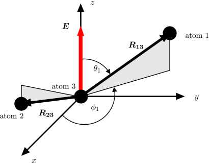
Figure 4: (Color online) Relative position vectors $\boldsymbol{R}_{13}$ and $\boldsymbol{R}_{23}$. In Eq. (4) of the main text, $\boldsymbol{R}_{\alpha 3}$ ($\alpha\in\{1,2\}$) is expressed in terms of spherical coordinates $R_{\alpha 3}$, $\theta_{\alpha}$ and $\phi_{\alpha}$. The angles $\theta_{1}$ and $\phi_{1}$ are indicated in the figure, while $\theta_{2}$ and $\phi_{2}$ were omitted in order to keep the drawing concise.

The new canonical momenta corresponding to the coordinates in Eq. (18) are given by

$$\boldsymbol{\hat{P}}_{\text{CM}}=\sum\limits_{\alpha=1}^{3}\boldsymbol{\hat{P}}_{\alpha},\quad\boldsymbol{\hat{p}}_{1}=\frac{2}{3}(\boldsymbol{\hat{P}}_{1}-\frac{1}{2}\boldsymbol{\hat{P}}_{2}-\frac{1}{2}\boldsymbol{\hat{P}}_{3}),$$ (19)

$$\boldsymbol{\hat{p}}_{2}=\frac{2}{3}(\boldsymbol{\hat{P}}_{2}-\frac{1}{2}\boldsymbol{\hat{P}}_{1}-\frac{1}{2}\boldsymbol{\hat{P}}_{3}).$$ (20)

The new coordinates and momenta obey canonical commutation relations

$$\left[\hat{R}_{\text{CM}}^{(i)},\hat{P}_{\text{CM}}^{(j)}\right]=\imath\hbar\delta_{ij},$$ (21)

$$\left[\hat{r}_{1}^{(i)},\hat{p}_{1}^{(j)}\right]=\imath\hbar\delta_{ij},\quad\left[\hat{r}_{2}^{(i)},\hat{p}_{2}^{(j)}\right]=\imath\hbar\delta_{ij},$$ (22)

where superscripts describe Cartesian components of the corresponding vectors and $\delta_{ij}$ is the Kronecker delta. All other commutators between coordinate and momentum components vanish. In the new coordinates and momenta, the system Hamiltonian can be written as

$$H_{\text{S}}=H_{\text{CM}}+H_{\text{rel}}+H,$$ (23)

where

$$H_{\text{CM}}=\frac{\boldsymbol{\hat{P}}_{\text{CM}}^{2}}{2(3m)}$$ (24)

is the centre-of-mass motion that we omit in the following. The kinetic energy of the relative motion is described by

$$H_{\text{rel}}=\frac{1}{2\mu}\boldsymbol{\hat{p}}_{1}^{2}+\frac{1}{2\mu}\boldsymbol{\hat{p}}_{2}^{2}+\frac{1}{2\mu}\boldsymbol{\hat{p}}_{1}\cdot\boldsymbol{\hat{p}}_{2},$$ (25)

where $\mu=m/2$ is the reduced two-body mass. Note that the last term in $H_{\text{rel}}$ mixes the two relative momenta. We combine all momentum components into one column vector

$$\boldsymbol{\hat{p}}=\left(\begin{array}[]{c}\boldsymbol{\hat{p}}_{1}\\ \boldsymbol{\hat{p}}_{2}\end{array}\right)$$ (28)

such that $H_{\text{rel}}$ can be written as

$$H_{\text{rel}}=\frac{1}{2\mu}\boldsymbol{\hat{p}}^{\text{t}}K\boldsymbol{\hat{p}},$$ (29)

where

$$K=\left(\begin{array}[]{cccccc}1&0&0&\frac{1}{2}&0&0\\ 0&1&0&0&\frac{1}{2}&0\\ 0&0&1&0&0&\frac{1}{2}\\ \frac{1}{2}&0&0&1&0&0\\ 0&\frac{1}{2}&0&0&1&0\\ 0&0&\frac{1}{2}&0&0&1\end{array}\right)$$ (36)

and the row vector $\boldsymbol{\hat{p}}^{\text{t}}$ is the transpose of $\boldsymbol{\hat{p}}$.

Next we determine the vibrational eigenmodes of the system in the trimer state $|\psi_{\text{t}}\rangle$. To this end, we combine all coordinates into one column vector

$$\boldsymbol{\hat{r}}=\left(\begin{array}[]{c}\boldsymbol{\hat{r}}_{1}\\ \boldsymbol{\hat{r}}_{2}\end{array}\right),$$ (39)

and its classical counterpart $\boldsymbol{r}$ contains the Cartesian coordinates of the relative position vectors $\boldsymbol{r}_{1}$ and $\boldsymbol{r}_{2}$. In particular, we denote the Cartesian coordinates of the local minimum of $\boldsymbol{\epsilon}_{\text{t}}$ by $\boldsymbol{r}_{\text{t}}$. We assume adiabatic motion in the internal state $|\psi_{\text{t}}\rangle$ and consider the harmonic part of the potential $\boldsymbol{\epsilon}_{\text{t}}$ near its minimum $\boldsymbol{r}_{\text{t}}$. With these approximations, the potential energy can be written as

$$V_{\text{pot}}=\frac{1}{2}\boldsymbol{\hat{x}}^{\text{t}}M\boldsymbol{\hat{x}},$$ (40)

where $\boldsymbol{\hat{x}}=\boldsymbol{\hat{r}}-\boldsymbol{r}_{\text{t}}\mathds{1}$ is the displacement from equilibrium and

$$M_{ij}=\frac{\partial^{2}}{\partial r^{(i)}\partial r^{(j)}}\left.\epsilon_{\text{t}}\right|_{\boldsymbol{r}_{\text{t}}}$$ (41)

are the Cartesian components of the Hessian matrix evaluated at $\boldsymbol{r}_{\text{t}}$. The eigenmodes and frequencies are thus determined by the Hamiltonian

$$H_{\text{osc}}=\frac{1}{2\mu}\boldsymbol{\hat{p}}^{\text{t}}K\boldsymbol{\hat{p}}+\frac{1}{2}\boldsymbol{\hat{x}}^{\text{t}}M\boldsymbol{\hat{x}}.$$ (42)

Here we follow the approach described in xiao:09 for the diagonalization of $H_{\text{osc}}$ and note that the matrix $K$ in Eq. (36) is positive definite, and hence a unique Cholesky decomposition of $K$ exists,

$$K=CC^{\text{t}},$$ (43)

where $C$ is a real and invertible matrix.

Figure 5: (Color online) Eigenmodes near the minimum of the potential curve $\epsilon_{\text{t}}$ in the laboratory frame. The arrows indicate the displacements of the position vectors $\boldsymbol{R}_{\alpha}$. The modes can be described as (a) symmetric stretch, (b) scissor, (c) asymmetric stretch, (d) wagging and (e) twisting. The modes in (b), (c) and (d), (e) are degenerate.

Note that the symmetric $6\times 6$ matrix $M$ is only positive semi-definite since $\boldsymbol{\epsilon}_{\text{t}}$ has not a strict minimum with respect to all six variables $\boldsymbol{r}$. In contrast to the five independent variables chosen in the main text, $\boldsymbol{r}$ can parametrize atomic configurations that leave $\boldsymbol{\epsilon}_{\text{t}}$ unchanged due to the azimuthal symmetry of the system. Next we introduce the matrix

$$L=C^{\text{t}}MC$$ (44)

which is real, symmetric and positive semi-definite. It can be diagonalized by an orthogonal transformation $S$,

$$S^{\text{t}}LS=\Omega,$$ (45)

where $\Omega=\mu\,\text{diag}(\omega_{1}^{2},\omega_{2}^{2},\ldots,\omega_{6}^{2})$ is a $6\times 6$ diagonal matrix. With the definition $A=CS$, Eqs. (43)-(45) imply

$$A^{-1}K[A^{-1}]^{\text{t}}=\mathds{1}_{6},\quad A^{\text{t}}MA=\Omega.$$ (46)

With the definitions

$$\boldsymbol{\hat{q}}=A^{-1}\boldsymbol{\hat{x}},\quad\boldsymbol{\hat{w}}=A^{\text{t}}\boldsymbol{\hat{p}},$$ (47)

we thus find that Eq. (42) can be written as

$$H_{\text{osc}}=\sum\limits_{i=1}^{6}\left(\frac{1}{2\mu}\left[\hat{w}^{(i)}\right]^{2}+\frac{1}{2}\mu\omega_{i}^{2}\left[\hat{q}^{(i)}\right]^{2}\right).$$ (48)

The commutation relations in Eq. (22) and $AA^{-1}=A^{-1}A=\mathds{1}_{6}$ ensure that $\boldsymbol{\hat{q}}$ and $\boldsymbol{\hat{w}}$ obey canonical commutation relations,

$$\left[\hat{q}^{(i)},\hat{w}^{(j)}\right]=\imath\hbar\delta_{ij},\quad\left[\hat{q}^{(i)},\hat{q}^{(j)}\right]=0,\quad\left[\hat{w}^{(i)},\hat{w}^{(j)}\right]=0.$$ (49)

Furthermore, Eqs. (43)-(45) allow us to derive the relation

$$A^{-1}KMA=\Omega.$$ (50)

It follows that the normal frequencies are determined by the eigenvalues of the matrix $KM$, and the eigenmodes are the corresponding eigenvectors which are the column vectors of $A$.

We find that the normal frequencies of the potential curve $\epsilon_{\text{t}}$ near its local minimum are given by

$$\omega_{1}=2.93\times\omega_{\text{vib}}, \omega_{2}=\omega_{3}=1.82\times\omega_{\text{vib}},$$

$$\omega_{4}=\omega_{5}=1.10\times\omega_{\text{vib}}, \omega_{6}=0,$$ (51)

where

$$\omega_{\text{vib}}=\sqrt{\frac{\hbar|\delta|}{\mu R_{0}^{2}}}.$$ (52)

In order to visualize the corresponding eigenmodes, we calculate the eigenvectors and employ the inverse relations of Eq. (18) to obtain the displacements of the atoms in the laboratory frame. The largest frequency $\omega_{1}=\omega_{\text{s}}$ belongs to the symmetric stretch mode shown in Fig. 5(a). The doubly degenerate frequency $\omega_{2}=\omega_{3}$ corresponds to the scissor and asymmetric stretch modes shown in Figs. 5(b) and (c), respectively. The two degenerate modes in Figs. 5(d) and (e) oscillate with frequency $\omega_{4}=\omega_{5}$ and describe wagging and twisting, respectively. Finally, the last mode with frequency $\omega_{6}=0$ corresponds to a circular motion of the three atoms in the $x-y$ plane and around their centre-of-mass.

A crucial assumption of our approach is that the dynamics in the trimer states remains adiabatic. Physically this is a reasonable assumption because the trimer states are well-separated in energy from the remaining states, see Fig. 2(c) of the main text. In addition, we have carried out semi-classical calculations in order to verify this assumption explicitly. To this end, we start from the full Hamiltonian $H_{\text{S}}$ (without $H_{\text{CM}}$) in Eq. (23) and derive a set of coupled equations for the mean values $\langle\boldsymbol{\hat{r}}\rangle$ and $\langle\boldsymbol{\hat{p}}\rangle$ tannoudji:lc ,

$$\partial_{t}\langle\boldsymbol{\hat{r}}\rangle =\frac{1}{\mu}K\langle\boldsymbol{\hat{p}}\rangle,$$

$$\partial_{t}\langle\boldsymbol{\hat{p}}\rangle =-\langle\nabla_{\boldsymbol{r}}H\rangle,$$

$$\imath\hbar\partial_{t}|\psi\rangle =H(\langle\boldsymbol{\hat{r}}\rangle)|\psi\rangle,$$ (53)

where $\nabla_{\boldsymbol{r}}=(\partial/\partial r^{(1)},\ldots,\partial/\partial r^{(6)})^{\text{t}}$ and $|\psi\rangle$ denotes the quantum state of the internal three-atom states. At $t=0$ we assume that the system is prepared in the trimer state $|\psi_{\text{t}}\rangle$ near the potential minimum and with initial momentum $\langle\boldsymbol{\hat{p}}\rangle_{0}$. Numerical integration of Eq. (53) yields $|\psi(t)\rangle$, and the overlap with the trimer state $|\psi_{\text{t}}\rangle$ at position $\langle\boldsymbol{\hat{r}}\rangle(t)$ is a direct measure of the adiabaticity of the evolution. We find that the evolution remains adiabatic to a very good approximation for various parameters and kinetic energies corresponding to several oscillation quanta $\hbar\omega_{\text{vib}}$.

IV Dimer states

The potential curves of two dipole-dipole interacting Rydberg atoms with the level scheme shown in Fig. 1(a) of the manuscript have been investigated in kiffner:12b . There are 16 dipole-dipole coupled $nsnp$ states shown in Fig. 6, where $R$ labels the distance between the atoms and both atoms are located in a plane perpendicular to the electric field $\boldsymbol{E}$.

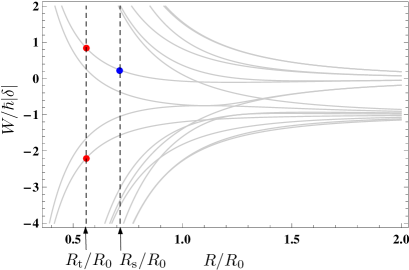
Figure 6: (Color online) All potential curves in the $nsnp$ subspace of two dipole-dipole coupled Rydberg atoms with the level scheme shown in Fig. 1(a) of the manuscript. The atoms are in the $x-y$ plane and $R$ is the atomic separation. See text for explanation of the blue and red dots.

Figure 6 illustrates that all potential curves are either strongly repulsive or attractive for $R_{\text{t}}=0.56\,R_{0}$ and $R_{\text{s}}=0.71\,R_{0}$, which establishes the Borromean nature of the trimer states. In general, the reduced density matrix $\rho_{\text{dimer}}$ of two atoms has an overlap with all 16 $nsnp$ states. The states corresponding to the potential curves indicated by the red dots contribute the most to $\rho_{\text{dimer}}$ (approximately 16% each) for the trimer state $|\psi_{\text{t}}\rangle$. The state corresponding to the potential curve indicated by the blue dot contributes the most to $\rho_{\text{dimer}}$ (approximately 21% ) for the trimer state $|\psi_{\text{s}}\rangle$.

References

- (1) M. Kiffner, W. Li, and D. Jaksch, Phys. Rev. Lett. 110, 170402 (2013)
- (2) R. P. Feynman, Phys. Rev. 56, 340 (1939)
- (3) M.-W. Xiao, arXiv:0908.0787.
- (4) See, e.g., chapter V.C.2 in: C. Cohen-Tannoudji, J. Dupont-Roc, and G. Grynberg, Atom- Photon Interactions (Wiley, New York, 1998).
- (5) M. Kiffner, H. Park, W. Li, and T. F. Gallagher, Phys. Rev. A 86, 031401(R) (2012)