Computational Complexity of
Smooth Differential Equations*

Abstract.

The computational complexity of the solution $h$ to the ordinary differential equation $h(0)=0$, $h^{\prime}(t)=g(t,h(t))$ under various assumptions on the function $g$ has been investigated. Kawamura showed in 2010 that the solution $h$ can be $\mathsf{PSPACE}$-hard even if $g$ is assumed to be Lipschitz continuous and polynomial-time computable. We place further requirements on the smoothness of $g$ and obtain the following results: the solution $h$ can still be $\mathsf{PSPACE}$-hard if $g$ is assumed to be of class $\mathrm{C}^{1}$; for each $k\geq 2$, the solution $h$ can be hard for the counting hierarchy even if $g$ is of class $\mathrm{C}^{k}$.

1. Introduction

Let $g\colon[0,1]\times\mathbf{R}\to\mathbf{R}$ be continuous and consider the differential equation

$$h(0) =0, Dh(t) =g(t,h(t))\quad t\in[0,1],$$ (1)

where $Dh$ denotes the derivative of $h$. How complex can the solution $h$ be, assuming that $g$ is polynomial-time computable? Here, polynomial-time computability and other notions of complexity are from the field of Computable Analysis [10, 20] and measure how hard it is to approximate real functions with specified precision (Section 3).

If we make no assumption on $g$ other than being polynomial-time computable, the solution $h$ (which is not unique in general) can be non-computable. Table 1 summarizes known results about the complexity of $h$ under various assumptions (that get stronger as we go down the table). In particular, as the third row says, if $g$ is (globally) Lipschitz continuous, then the (unique) solution $h$ is known to be polynomial-space computable but still can be $\mathsf{PSPACE}$-hard [4]. In this paper, we study the complexity of $h$ when we put stronger assumptions about the smoothness of $g$.

Table 1. Complexity of the solution $h$ of (1) assuming $g$ is polynomial-time computable

Assumptions	Upper bounds	Lower bounds
—	—	can be all non-computable [15]
$h$ is the unique solution	computable [2]	can take arbitrarily long time [9, 12]
the Lipschitz condition	polynomial-space [9]	can be $\mathsf{PSPACE}$-hard [4]
$g$ is of class $\mathrm{C}^{(\infty,1)}$	polynomial-space	can be $\mathsf{PSPACE}$-hard (Theorem 1)
$g$ is of class $\mathrm{C}^{(\infty,k)}$ (for each constant $k$)	polynomial-space	can be $\mathsf{CH}$-hard (Theorem 2)
$g$ is analytic	polynomial-time [13, 11, 3]	—

In numerical analysis, knowledge about smoothness of the input function (such as being differentiable enough times) often helps to apply certain algorithms or simplify their analysis. However, to our knowledge, this casual understanding that smoothness is good has not been rigorously substantiated in terms of computational complexity theory. This motivates us to ask whether, for our differential equation (1), smoothness really reduces the complexity of the solution.

At one extreme is the case where $g$ is analytic: $h$ is then polynomial-time computable (the last row of the table) by an argument based on Taylor series (this does not necessarily mean that computing the values of $h$ from those of $g$ is easy; see the last paragraph of Section 5.2). Thus our interest is in the cases between Lipschitz and analytic (the fourth and fifth rows). We say that $g$ is of class $\mathrm{C}^{(i,j)}$ if the partial derivative $D^{(n,m)}g$ (often also denoted $\partial^{n+m}g(t,y)/\partial t^{n}\partial y^{m}$) exists and is continuous for all $n\leq i$ and $m\leq j$; it is said to be of class $\mathrm{C}^{(\infty,j)}$ if it is of class $\mathrm{C}^{(i,j)}$ for all $i\in\mathbf{N}$.

We will show that adding continuous differentiability does not break the $\mathsf{PSPACE}$-completeness that we knew from [4] for the Lipschitz continuous case:

Theorem 1.

There exists a polynomial-time computable function $g\colon[0,1]\times[-1,1]\to\mathbf{R}$ of class $\mathrm{C}^{(\infty,1)}$ such that the equation (1) has a $\mathsf{PSPACE}$-hard solution $h\colon[0,1]\to\mathbf{R}$.

The complexity notions (computability and hardness) in this and the following theorems will be explained in Section 3. When $g$ is more than once differentiable, we did not quite succeed in proving that $h$ is $\mathsf{PSPACE}$-hard in the same sense, but we will prove it $\mathsf{CH}$-hard, where $\mathsf{CH}\subseteq\mathsf{PSPACE}$ is the counting hierarchy (see Section 2):

Theorem 2.

Let $k$ be a positive integer. There is a polynomial-time computable function $g\colon[0,1]\times[-1,1]\to\mathbf{R}$ of class $\mathrm{C}^{(\infty,k)}$ such that the equation (1) has a $\mathsf{CH}$-hard solution $h\colon[0,1]\to\mathbf{R}$.

In Theorems 1 and 2, we said $g\colon[0,1]\times[-1,1]\to\mathbf{R}$ instead of $g\colon[0,1]\times\mathbf{R}\to\mathbf{R}$, because the notion of polynomial-time computability of real functions in this paper is defined only when the domain is a bounded closed region. This makes the equation (1) ill-defined in case $h$ ever takes a value outside $[-1,1]$. By saying that $h$ is a solution in Theorem 1, we are also claiming that $h(t)\in[-1,1]$ for all $t\in[0,1]$. This is no essential restriction, because any pair of functions $g\colon[0,1]\times\mathbf{R}\to\mathbf{R}$ and $h\colon[0,1]\to\mathbf{R}$ satisfying the equation could be scaled down in an appropriate way (without affecting the computational complexity) to make $h$ stay in $[-1,1]$. In any case, since we are making stronger assumptions on $g$ than Lipschitz continuity, the solution $h$, if it exists, is unique.

Whether smoothness of the input function reduces the complexity of the output has been studied for operators other than solving differential equations, and the following negative results are known. The integral of a polynomial-time computable real function can be $\mathsf{\#P}$-hard, and this does not change by restricting the input to $\mathrm{C}^{\infty}$ (infinitely differentiable) functions [10, Theorem 5.33]. Similarly, the function obtained by maximization from a polynomial-time computable real function can be $\mathsf{NP}$-hard, and this is still so even if the input function is restricted to $\mathrm{C}^{\infty}$ [10, Theorem 3.7]. (Restricting to analytic inputs renders the output polynomial-time computable, again by the argument based on Taylor series.) In contrast, for the differential equation we only have Theorem 2 for each $k$, and do not have any hardness result when $g$ is assumed to be infinitely differentiable.

Theorems 1 and 2 are about the complexity of each solution $h$. We will also discuss the complexity of the final value $h(1)$ and the complexity of the operator that maps $g$ to $h$; see Sections 5.1 and 5.2.

Notation

Let $\mathbf{N}$, $\mathbf{Z}$, $\mathbf{Q}$, $\mathbf{R}$ denote the set of natural numbers, integers, rational numbers and real numbers, respectively.

We assume that any polynomial is increasing, since it does not change the meaning of polynomial-time computable or polynomial-space computable.

Let $A$ and $B$ be bounded closed intervals in $\mathbf{R}$. We write $|f|=\sup_{x\in A}f(x)$ for $f\colon A\to\mathbf{R}$. A function $f\colon A\to\mathbf{R}$ is of class $\mathrm{C}^{i}$ (or $i$-times continuously differentiable) if all the derivatives $Df,D^{2}f,\dots,D^{i}f$ exist and are continuous.

For a function $g$ of two variables, we write $D_{1}g$ and $D_{2}g$ for the derivatives of $g$ with respect to the first and the second variable, respectively, when they exist. A function $g\colon A\times B\to\mathbf{R}$ is of class $\mathrm{C}^{(i,j)}$ if for each $m\in\{0,\dots,i\}$ and $n\in\{0,\dots j\}$, the derivative $D_{1}^{m}D_{2}^{n}g$ exists and is continuous. This derivative $D_{1}^{m}D_{2}^{n}g$ is then written $D^{(m,n)}g$ (and is known to equal $D_{e_{1}}\ldots D_{e_{m+n}}g$ for any sequence $e_{1}\ldots e_{m+n}$ of $m$ $1$s and $n$ $2$s). A function $g$ is of class $\mathrm{C}^{(\infty,j)}$ if it is of class $\mathrm{C}^{(i,j)}$ for all $i\in\mathbf{N}$.

2. The Counting Hierarchy

We assume that the reader is familiar with the basics of complexity theory, such as the classes $\mathsf{P}$ and $\mathsf{PSPACE}$ and the notions of reduction and hardness [19]. We briefly review the class $\mathsf{CH}$.

The counting hierarchy $\mathsf{CH}$ is defined analogously to the polynomial-time hierarchy $\mathsf{PH}$ [19, Kapitel 10.4] using oracle machines corresponding to the class $\mathsf{PP}$ [19, Kapitel 3.3] instead of $\mathsf{NP}$: thus, $\mathsf{CH}=\bigcup_{n\in\mathbf{N}}\mathsf{C}_{n}\mathsf{P}$, where each level $\mathsf{C}_{n}\mathsf{P}$ is defined inductively by $\mathsf{C}_{0}\mathsf{P}=\mathsf{P}$ and $\mathsf{C}_{n+1}\mathsf{P}=\mathsf{PP}^{\mathsf{C}_{n}\mathsf{P}}$. We leave the details of this definition to the original papers [18, 14, 17]. All we need for our purpose is the fact (Lemma 3 below) that $\mathsf{C}_{n}\mathsf{P}$ is characterized by the following complete problem $\mathsf{C}_{n}B_{\mathrm{be}}$: given $n$ lists $X_{1}$, …, $X_{n}$ of propositional variables, a propositional formula $\phi(X_{1},\dots,X_{n})$ with all free variables listed, and numbers $m_{1}$, …, $m_{n}$ in binary, determine whether

$$\mathsf{C}^{m_{n}}{X_{n}}\ldots\mathsf{C}^{m_{1}}{X_{1}}\phi(X_{1},\dots,X_{n})$$ (2)

is true. Here, $\mathsf{C}^{m}$ is the counting quantifier: for every formula $\phi(X)$ with the list $X$ of $l$ free variables, we write

$$\mathsf{C}^{m}X\phi(X)\iff\sum_{x\in\{0,1\}^{l}}\phi(x)\geq m,$$ (3)

where formula $\phi$ is identified with the function $\phi\colon\{0,1\}^{l}\to\{0,1\}$ such that $\phi(X)=1$ when $\phi(X)$ is true.

Lemma 3 ([18, Theorem 7]).

For every $n\geq 1$, the problem $\mathsf{C}_{n}B_{\mathrm{be}}$ is $\mathsf{C}_{n}\mathsf{P}$-complete.

By this, we mean that any problem $A$ in $\mathsf{C}_{n}\mathsf{P}$ reduces to $\mathsf{C}_{n}B_{\mathrm{be}}$ via some polynomial-time function $F$ in the sense that $v\in A$ if and only if $F(v)\in\mathsf{C}_{n}B_{\mathrm{be}}$.

Note that this is analogous to the polynomial hierarchy $\mathsf{PH}$, whose $n$th level $\mathsf{\Sigma}^{p}_{n}$ has the complete problem that asks for the value of a formula of the form $\exists X_{n}\forall X_{n-1}\exists X_{n-2}\ldots\allowbreak\phi(X_{1},\dots,X_{n})$ with $n$ alternations of universal and existential quentifiers. Note also that the counting quantifier generalizes the universal and existential quentifiers, and hence $\mathsf{PH}\subseteq\mathsf{CH}$ – in fact, it is known [16] that $\mathsf{PH}$ is contained already in $\mathsf{P}^{\mathsf{PP}}$ and thus in the second level of the counting hierarchy.

3. Computational Complexity of Real Functions

We review some complexity notions from Computable Analysis [10, 20]. We start by fixing an encoding of real numbers by string functions.

Definition 4.

A function $\phi\colon\{0,1\}^{*}\to\{0,1\}^{*}$ is a name of a real number $x$ if for all $n\in\mathbf{N}$, $\phi(0^{n})$ is the binary representation of $\lfloor x\cdot 2^{n}\rfloor$ or $\lceil x\cdot 2^{n}\rceil$, where $\lfloor\cdot\rfloor$ and $\lceil\cdot\rceil$ mean rounding down and up to the nearest integer.

In effect, a name of a real number $x$ takes each string $0^{n}$ to an approximation of $x$ with precision $2^{-n}$.

We use oracle Turing machines (henceforth just machines) to work on these names (Fig. 1). Let $M$ be a machine and $\phi$ be a function from strings to strings. We write $M^{\phi}(0^{n})$ for the output string when $M$ is given $\phi$ as oracle and string $0^{n}$ as input. Thus we also regard $M^{\phi}$ as a function from strings to strings.

Figure 1. A machine $M$ computing a real function $f$

Definition 5.

Let $A$ be a bounded closed interval of $\mathbf{R}$. A machine $M$ computes a real function $f\colon A\to\mathbf{R}$ if for any $x\in A$ and any name $\phi_{x}$ of it, $M^{\phi_{x}}$ is a name of $f(x)$.

Computation of a function $f\colon A\to\mathbf{R}$ on a two-dimensional bounded closed region $A\subseteq\mathbf{R}^{2}$ is defined similarly using machines with two oracles.

A real function is (polynomial-time) computable if there exists some machine that computes it (in polynomial time). Polynomial-time computability of a real function $f$ means that for any $n\in\mathbf{N}$, an approximation of $f(x)$ with error bound $2^{-n}$ is computable in time polynomial in $n$ independent of the real number $x$.

By the time the machine outputs the approximation of $f(x)$ of precision $2^{-n}$, it knows $x$ only with some precision $2^{-m}$. This implies that all computable real functions are continuous. If the machine runs in polynomial time, this $m$ is bounded polynomially in $n$. This implies (5) in the following lemma, which characterizes polynomial-time real functions by the usual polynomial-time computability of string functions without using oracle machines.

Lemma 6.

A real function is polynomial-time computable if and only if there exist a polynomial-time computable function $\phi\colon(\mathbf{Q}\cap[0,1])\times\{0,1\}^{*}\to\mathbf{Q}$ and polynomial $p\colon\mathbf{N}\to\mathbf{N}$ such that for all $d\in\mathbf{Q}\cap[0,1]$ and $n\in\mathbf{N}$,

$$|\phi(d,0^{n})-f(d)|\leq 2^{-n},$$ (4)

and for all $x,y\in[0,1]$, $n\in\mathbf{N}$,

$$|x-y|\leq 2^{-p(n)}\Rightarrow|f(x)-f(y)|\leq 2^{-n},$$ (5)

where each rational number is written as a fraction whose numerator and denominator are integers in binary.

To speak about hardness of a real function, we define the notion of a language to it. A language $L\subseteq\{0,1\}^{*}$ is identified with the function $L\colon\{0,1\}^{*}\to\{0,1\}$ such that $L(u)=1$ when $u\in L$.

Definition 7.

A language $L$ reduces to a function $f\colon[0,1]\to\mathbf{R}$ if there exist a polynomial-time function $S$ and a polynomial-time oracle Turing machine $M$ (Fig. 2) such that for any string $u$,

1. $S(u,\cdot)$ is a name of a real number $x_{u}$, and

2. for any name $\phi$ of $f(x_{u})$, we have that $M^{\phi}(u)$ accepts if and only if $u\in L$.

This reduction may superficially look stronger (and hence the reducibility weaker) than the one in Kawamura [4] in that $M$ can make multiple queries adaptively, but it is not hard to see that this makes no difference.

For a complexity class $C$, a function $f$ is $C$-hard if all languages in $C$ reduce to $f$.

Figure 2. Reduction from a language $L$ to a function $f\colon[0,1]\to\mathbf{R}$

4. Proof of the Main Theorems

The proofs of Theorems 1 and 2 proceed as follows. In Section 4.1, we define difference equations, a discrete version of the differential equations. We show that these equations with certain restrictions are $\mathsf{PSPACE}$- and $\mathsf{CH}$-hard. In Section 4.2, we show that these classes of difference equations can be simulated by families of differential equations satisfying certain uniform bounds on higher-order derivatives. In Section 4.3, we prove Theorems 1 and 2 by putting these families of functions together to obtain one differential equation with the desired smoothness ($\mathrm{C}^{(\infty,1)}$ and $\mathrm{C}^{(\infty,k)}$).

The idea of simulating a discrete system with limited feedback by differential equations was essentially already present in the proof of the Lipschitz version of these results [4]. We look more closely at this limitation on feedback, and express it as a restriction on the height of the difference equation. We show that a stronger height restriction allows the difference equation to be simulated by smoother differential equations (see the proof of Lemma 10 and the discussion after it), leading to the $\mathsf{CH}$-hardness for $\mathrm{C}^{(\infty,k)}$ functions.

4.1. Difference equations

In this section, we define difference equations, which are a discrete version of differential equations. Then we show the $\mathsf{PSPACE}$- and $\mathsf{CH}$-hardness of families of difference equations with different height restrictions.

Let $[n]$ denote $\{0,\dots,n-1\}$. Let $G\colon[P]\times[Q]\times[R]\to\{-1,0,1\}$ and $H\colon[P+1]\times[Q+1]\to[R]$. We say that $H$ is the solution of the difference equation given by $G$ if for all $i\in[P]$ and $T\in[Q]$ (Fig. 3),

$$H(i,0)=H(0,T)=0,$$ (6)

$$H(i+1,T+1)-H(i+1,T)=G(i,T,H(i,T)).$$ (7)

We call $P$, $Q$ and $R$ the height, width and cell size of the difference equation. The equations (6) and (7) are similar to the initial condition $h(0)=0$ and the equation $Dh(t)=g(t,h(t))$ in (1), respectively. In Section 4.2, we will use this similarity to simulate difference equations by differential equations.

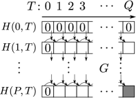
Figure 3. The solution $H$ of the difference equation given by $G$

We view a family of difference equations as a computing system by regarding the value of the bottom right cell (the gray cell in Fig. 3) as the output. A family $(G_{u})_{u}$ of functions $G_{u}\colon[P_{u}]\times[Q_{u}]\times[R_{u}]\to\{-1,0,1\}$ recognizes a language $L$ if for each $u$, the difference equation given by $G_{u}$ has a solution $H_{u}$ and $H_{u}(P_{u},Q_{u})=L(u)$. A family $(G_{u})_{u}$ is uniform if the height, width and cell size of $G_{u}$ are polynomial-time computable from $u$ (in particular, they must be bounded by $2^{p(|u|)}$, for some polynomial $p$) and $G_{u}(i,T,Y)$ is polynomial-time computable from $(u,i,T,Y)$. A family $(G_{u})_{u}$ has polynomial height (and logarithmic height, respectively) if the height $P_{u}$ is bounded by $|u|^{\mathrm{O}(1)}$ (and by $\mathrm{O}(\log|u|)$, respectively). With this terminology, the key lemma in [4, Lemma 4.7] can be written as follows:

Lemma 8.

There exists a $\mathsf{PSPACE}$-hard language $L$ that is recognized by some uniform family of functions with polynomial height.

Kawamura [4] obtained the hardness result in the third row of Table 1 by simulating the difference equations of Lemma 8 by Lipschitz continuous differential equations. Likewise, Theorem 1 follows from Lemma 8 by a modified construction that keeps the function in class $\mathrm{C}^{(\infty,1)}$ (Sections 4.2 and 4.3).

We show further that difference equations restricted to logarithmic height can be simulated by $\mathrm{C}^{(\infty,k)}$ functions for each $k$ (Sections 4.2 and 4.3). Theorem 2 follows from this simulation and the following lemma.

Lemma 9.

There exists a $\mathsf{CH}$-hard language $L$ that is recognized by some uniform family of functions with logarithmic height.

Proof.

We define the desired language $L$ by

$$\langle 0^{2^{n}},w\rangle\in L\iff w\in\mathsf{C}_{n}B_{\mathrm{be}},$$ (8)

using the $\mathsf{C}_{n}\mathsf{P}$-hard language $\mathsf{C}_{n}B_{\mathrm{be}}$ from Lemma 3. Then $L$ is obviously $\mathsf{CH}$-hard.

We construct a logarithmic-height uniform function family $(G_{u})_{u}$ recognizing $L$. We will describe how to construct $G_{u}$ for a string $u$ of the form $\langle 0^{2^{n}},\allowbreak\langle\phi(X_{1},\dots,X_{n}),m_{1},\dots,m_{n}\rangle\rangle$, where $\phi$ is a formula, and $X_{1}$, …, $X_{n}$ are lists of variables with lengths $m_{1}$, …, $m_{n}$, respectively.

We write $l_{i}=|X_{i}|$ and $s_{i}=\sum^{i}_{j=1}(l_{j}+1)$. For each $i\in\{0,\dots,n\}$ and $x_{i+1}\in\{0,1\}^{l_{i+1}},\dots,x_{n}\in\{0,1\}^{l_{n}}$, we write $\phi_{i}(x_{i+1},\dots,x_{n})$ for the truth value ($1$ or $0$) of $\mathsf{C}^{m_{i}}{X_{i}}\ldots\allowbreak\mathsf{C}^{m_{1}}{X_{1}}\allowbreak\phi(X_{1},\dots,X_{i},x_{i+1},\dots,x_{n})$. Note that $\phi_{0}(x_{1},\ldots,x_{n})=\phi(x_{1},\ldots,x_{n})$, $\phi_{n}()=L(u)$, and the relation between $\phi_{i-1}$ and $\phi_{i}$ is given by

$$\phi_{i}(x_{i+1},\dots,x_{n})=C^{m_{i}}\Bigl{(}\sum_{x_{i}\in\{0,1\}^{l_{i}}}\phi_{i-1}(x_{i},x_{i+1},\dots,x_{n})\Bigr{)},$$ (9)

where we define $C^{m}\colon\mathbf{N}\to\{0,1\}$ by

$$C^{m}(k)=\begin{cases}1&\text{if}\ k\geq m,\\ 0&\text{if}\ k<m.\end{cases}$$ (10)

For $T\in\mathbf{N}$, we write $T_{i}$ for the $i$th digit of $T$ written in binary ($T_{0}$ being the least significant digit), and $T_{[i,j]}$ for the string $T_{j-1}T_{j-2}\cdots T_{i+1}T_{i}$.

For each $(i,T,Y)\in[n+1]\times[2^{s_{n}}+1]\times[2^{|u|}]$, we define $G_{u}(i,T,Y)$ as follows. The first row is given by

$$G_{u}(0,T,Y)=(-1)^{T_{s_{1}}}\phi(T_{[1,s_{1}]},T_{[s_{1}+1,s_{2}]},\dots,T_{[s_{n-1}+1,s_{n}]}),$$ (11)

and for $i\neq 0$, we define

$$G_{u}(i,T,Y)=\begin{cases}(-1)^{T_{s_{i+1}}}C^{m_{i}}(Y)&\text{if}\ T_{[1,s_{i}+1]}=10\cdots 0,\\ 0&\text{otherwise}.\end{cases}$$ (12)

This family $(G_{u})_{u}$ is clearly uniform, and its height $n+1$ is logarithmic in $|u|$.

Let $H_{u}$ be the solution (as defined in (6) and (7)) of the difference equation given by $G_{u}$. We prove by induction on $i$ that $H_{u}(i,T)\in[2^{l_{i}}+1]$ for all $T$, and that

$$G_{u}(i,V,H_{u}(i,V))=(-1)^{V_{s_{i+1}}}\phi_{i}(V_{[s_{i}+1,s_{i+1}]},\dots,V_{[s_{n-1}+1,s_{n}]})$$ (13)

if $V_{[1,s_{i}+1]}=10\cdots 0$ (otherwise it is immediate from the definition that $G_{u}(i,V,H_{u}(n,V))=0$). For $i=0$, the claims follow from (11). For $i>0$, suppose that the induction hypothesis

$$G_{u}(i-1,V,H_{u}(i-1,V))=(-1)^{V_{s_{i}}}\phi_{i-1}(V_{[s_{i-1}+1,s_{i}]},\dots,V_{[s_{n-1}+1,s_{n}]})$$ (14)

holds. Since $H_{u}$ is the solution of the difference equation given by $G_{u}$, we have

$$H_{u}(i,T)=\sum_{V=0}^{T-1}G_{u}(i-1,V,H_{u}(i-1,V)).$$ (15)

Since the assumption (14) implies that flipping the bit $V_{s_{i}}$ of any $V$ reverses the sign of $G_{u}(i-1,V,H_{u}(i-1,V))$, most of the summands in (15) cancel out. The only nonzero terms that can survive are the ones corresponding to those $V$ that satisfy $V_{[1,s_{i-1}+1]}=10\cdots 0$ and lie between the numbers whose binary representations are $T_{s_{n}}\dots T_{s_{i}+1}00\dots 0$ and $T_{s_{n}}\dots T_{s_{i}+1}01\dots 1$. There are at most $2^{l_{i}}$ such terms, and each of them is $0$ or $1$, so $H_{u}(i,T)\in[2^{l_{i}}+1]$. In particular, if $V_{[1,s_{i}+1]}=10\cdots 0$, we have

$$H_{u}(i,V)=\sum_{x\in\{0,1\}^{l_{i}}}\phi_{i-1}(x,V_{[s_{i}+1,s_{i+1}]},\dots,V_{[s_{n-1}+1,s_{n}]}).$$ (16)

By this and (9), we have

$$C^{m_{i}}(H_{u}(i,V))=\phi_{i}(V_{[s_{i}+1,s_{i+1}]},\dots,V_{[s_{n-1}+1,s_{n}]}).$$ (17)

By this and (12), we have (13), completing the induction step.

By substituting $n$ for $i$ and $2^{s_{n}}$ for $V$ in (13), we get $G_{u}(n,2^{s_{n}},H_{u}(n,2^{s_{n}}))=\phi_{n}()=L(u)$. Hence $H_{u}(n+1,2^{s_{n}}+1)=L(u)$. ∎

Note that for $\mathsf{CH}$-hardness, we could have defined $L$ using a faster growing function than $2^{n}$ in (8). This would allow the difference equation in Lemma 9 to have height smaller than logarithmic. We stated Lemma 9 with logarithmic height, simply because this was the highest possible difference equations that we were able to simulate by $\mathrm{C}^{(\infty,k)}$ functions (in the proof of Lemma 10 below).

4.2. Simulating difference equations by real functions

We show that certain families of smooth differential equations can simulate $\mathsf{PSPACE}$- and $\mathsf{CH}$-hard difference equations from the previous section.

Before stating Lemmas 10 and 11, we extend the definition of polynomial-time computability of real functions to that of families of real functions. A machine $M$ computes a family $(f_{u})_{u}$ of functions $f_{u}\colon A\to\mathbf{R}$ indexed by strings $u$ if for any $x\in A$ and any name $\phi_{x}$ of $x$, the function taking $v$ to $M^{\phi_{x}}(u,v)$ is a name of $f_{u}(x)$. We say a family of real functions $(f_{u})_{u}$ is polynomial-time if there is a polynomial-time machine computing $(f_{u})_{u}$.

Lemma 10.

There exist a $\mathsf{CH}$-hard language $L$ and a polynomial $\mu$, such that for any $k\geq 1$ and polynomial $\gamma$, there are a polynomial $\rho$ and families $(g_{u})_{u}$, $(h_{u})_{u}$ of real functions such that $(g_{u})_{u}$ is polynomial-time computable and for any string $u$:

1. $g_{u}\colon[0,1]\times[-1,1]\to\mathbf{R}$, $h_{u}\colon[0,1]\to[-1,1]$;

2. $h_{u}(0)=0$ and $Dh_{u}(t)=g_{u}(t,h_{u}(t))$ for all $t\in[0,1]$;

3. $g_{u}$ is of class $\mathrm{C}^{(\infty,k)}$;

4. $D^{(i,0)}g_{u}(0,y)=D^{(i,0)}g_{u}(1,y)=0$ for all $i\in\mathbf{N}$ and $y\in[-1,1]$;

5. $\left|D^{(i,j)}g_{u}(t,y)\right|\leq 2^{\mu(i,|u|)-\gamma(|u|)}$ for all $i\in\mathbf{N}$ and $j\in\{0,\dots,k\}$;

6. $h_{u}(1)=2^{-\rho(|u|)}L(u)$.

Lemma 11.

There exist a $\mathsf{PSPACE}$-hard language $L$ and a polynomial $\mu$, such that for any polynomial $\gamma$, there are a polynomial $\rho$ and families $(g_{u})_{u}$, $(h_{u})_{u}$ of real functions such that $(g_{u})_{u}$ is polynomial-time computable and for any string $u$ satisfying (i)–(vi) of Lemma 10 with $k=1$.

In Lemmas 10 and 11, we have the new conditions (iii)–(v) about the smoothness and the derivatives of $g_{u}$ that were not present in [4, Lemma 4.1]. To satisfy these conditions, we construct $g_{u}$ using the smooth function $f$ in following lemma.

Lemma 12 ([10, Lemma 3.6]).

There exist a polynomial-time function $f\colon[0,1]\to\mathbf{R}$ of class $\mathrm{C}^{\infty}$ and a polynomial $s$ such that

• $f(0)=0$ and $f(1)=1$;

• $D^{n}f(0)=D^{n}f(1)=0$ for all $n\geq 1$;

• $f$ is strictly increasing;

• $D^{n}f$ is polynomial-time computable for all $n\geq 1$;

• $|D^{n}f|\leq 2^{s(n)}$ for all $n\geq 1$.

Although the existence of the polynomial $s$ was not explicitly stated in [10, Lemma 3.6], it can be proved easily.

We will prove Lemma 10 using Lemma 9 as follows. Let $(G_{u})_{u}$ be a family of functions obtained by Lemma 9, and let $(H_{u})_{u}$ be the family of the solutions of the difference equations given by $(G_{u})_{u}$. We construct $h_{u}$ and $g_{u}$ from $H_{u}$ and $G_{u}$ so that $h_{u}(T/2^{q(|u|)})=\sum^{p(|u|)}_{i=0}H_{u}(i,T)/B^{d_{u}(i)}$ for each $T=0$, …, $2^{q(|u|)}$ and $Dh_{u}(t)=g_{u}(t,h_{u}(t))$. The polynomial-time computability of $(g_{u})_{u}$ follows from that of $(G_{u})_{u}$. We omit the analogous and easier proof of Lemma 11.

Proof of Lemma 10.

Let $L$ and $(G_{u})_{u}$ be as in Lemma 9, and let $H_{u}$ be the solutions of the difference equations given by $G_{u}$. Let $f$ and $s$ be as in Lemma 12.

We may assume that $G_{u}\colon[p(|u|)]\times[2^{q(|u|)}]\times[2^{r(|u|)}]\to\{-1,0,1\}$ for some $p$, $q$, $r\colon\mathbf{N}\to\mathbf{N}$, where $p$ has logarithmic growth and $q$ and $r$ are polynomials. We may also assume, similarly to the beginning of the proof of [4, Lemma 4.1], that

$$H_{u}(i,2^{q(|u|)})=\begin{cases}L(u)&\text{if}\ i=p(|u|),\\ 0&\text{if}\ i<p(|u|),\end{cases}$$ (18)

$$G_{u}(i,T,Y)\neq 0\to i=j_{u}(T)$$ (19)

for some $j_{u}\colon[2^{q(\lvert u\rvert)}]\to[p(\lvert u\rvert)]$.

We construct families of real functions $(g_{u})_{u}$ and $(h_{u})_{u}$ that simulate $G_{u}$ and $H_{u}$ in the sense that $h_{u}(T/2^{q(|u|)})=\sum^{p(|u|)}_{i=0}H_{u}(i,T)/B^{d_{u}(i)}$, where the constant $B$ and the (increasing) function $d_{u}\colon[p(|u|)+1]\to\mathbf{N}$ are defined by

$$B =2^{\gamma(|u|)+r(|u|)+s(k)+k+3}, d_{u}(i) =\begin{cases}(k+1)^{i}&\text{if}\ i<p(|u|),\\ \sigma(|u|)&\text{if}\ i=p(|u|),\end{cases}$$ (20)

where $\sigma$ is a polynomial satisfying $(k+1)^{p(x)}\leq\sigma(x)$ (which exists because $p$ is logarithmic). Thus, the value $H_{u}(i,T)\in[2^{r(\lvert u\rvert)}]$ will be stored in the $d_{u}(i)$th digit of the base-$B$ expansion of the real number $h_{u}(T/2^{q(\lvert u\rvert)})$. This exponential spacing described by $d_{u}$ will be needed when we bound the derivative $D^{(i,j)}g_{u}$ in (4.2) below.

For each $(t,y)\in[0,1]\times[-1,1]$, there exist unique $N\in\mathbf{N}$, $\theta\in[0,1)$, $Y\in\mathbf{Z}$ and $\eta\in[-1/4,3/4)$ such that $t=(T+\theta)2^{-q(|u|)}$ and $y=(Y+\eta)B^{-d_{u}(j_{u}(T))}$. Using $f$ and a polynomial $s$ of Lemma 12, we define $\tilde{g}_{u,Y}\colon[0,1]\to\mathbf{R}$, $g_{u}\colon[0,1]\times[-1,1]\to\mathbf{R}$ and $h_{u}\colon[0,1]\to[-1,1]$ by

$$\tilde{g}_{u,Y}(t) =\frac{2^{q(|u|)}Df(\theta)}{B^{d_{u}(j_{u}(T)+1)}}G_{u}\bigl{(}j_{u}(T),T,Y\bmod 2^{r(|u|)}\bigr{)},$$ (21)

$$g_{u}(t,y) =\begin{cases}\tilde{g}_{u,Y}(t)&\text{if }\eta\leq\frac{1}{4},\\ (1-f(\frac{4\eta-1}{2}))\tilde{g}_{u,Y}(t)+f(\frac{4\eta-1}{2})\tilde{g}_{u,Y+1}(t)&\text{if }\eta>\frac{1}{4},\end{cases}$$ (22)

$$h_{u}(t) =\sum^{p(|u|)}_{i=0}\frac{H_{u}(i,T)}{B^{d_{u}(i)}}+\frac{f(\theta)}{B^{d_{u}(j_{u}(T)+1)}}G_{u}\bigl{(}j_{u}(T),T,H_{u}(j_{u}(T),T)\bigr{)}.$$ (23)

We will verify that $(g_{u})_{u}$ and $(h_{u})_{u}$ defined above satisfy all the conditions stated in Lemma 10. Polynomial-time computability of $(g_{u})_{u}$ can be verified using Lemma 6. The condition (i) is immediate, and (ii) follows from the relation between $G_{u}$ and $H_{u}$ (by a similar argument to [4, Lemma 4.1]).

Since $g_{u}$ is constructed by interpolating between the (finitely many) values of $G_{u}$ using a $\mathrm{C}^{(\infty,\infty)}$ function $f$, it is of class $\mathrm{C}^{(\infty,\infty)}$ and thus satisfies (iii). Calculating from (21), we have

$$D^{i}\tilde{g}_{u,Y}(t)=\frac{2^{(i+1)q(|u|)}D^{i+1}f(\theta)}{B^{d_{u}(j_{u}(T)+1)}}G_{u}\bigl{(}j_{u}(T),T,Y\bmod 2^{r(|u|)}\bigr{)}$$ (24)

for each $i\in\mathbf{N}$. By this and (22), we have

$$D^{(i,0)}g_{u}(t,y)=\begin{cases}D^{i}\tilde{g}_{u,Y}(t)&\text{if}\ \eta\leq\frac{1}{4},\\ \bigl{(}1-f\bigl{(}\frac{4\eta-1}{2}\bigr{)}\bigr{)}D^{i}\tilde{g}_{u,Y}(t)+f\bigl{(}\frac{4\eta-1}{2}\bigr{)}D^{i}\tilde{g}_{u,Y+1}(t)&\text{if}\ \frac{1}{4}<\eta\end{cases}$$ (25)

for each $i\in\mathbf{N}$ and

$$D^{(i,j)}g_{u}(t,y)=\begin{cases}0&\text{if}\ {-\frac{1}{4}}<\eta<\frac{1}{4},\\ \bigl{(}2B^{d_{u}(j_{u}(T))}\bigr{)}^{j}\cdot D^{j}f\bigl{(}\frac{4\eta-1}{2}\bigr{)}\cdot(D^{i}\tilde{g}_{u,Y+1}(t)-D^{i}\tilde{g}_{u,Y}(t))&\text{if}\ \frac{1}{4}<\eta<\frac{3}{4}\end{cases}$$ (26)

for each $i\in\mathbf{N}$ and $j\in\{1,\dots,k\}$. Substituting $t=0,1$ ($\theta=0$) into (25), we get $D^{(i,0)}g_{u}(0,y)=D^{(i,0)}g_{u}(1,y)=0$, as required in (iv).

We show that (v) holds with $\mu(x,y)=(x+1)q(y)+s(x+1)$. Note that $\mu$ is a polynomial independent of $k$ and $\gamma$, and that $|D^{i}\tilde{g}_{u,Y}(t)|\leq 2^{\mu(i,\lvert u\rvert)}/B^{d_{u}(j_{u}(T)+1)}$ by (24). Hence,

$$|D^{(i,j)}g_{u}(t,y)| \leq\bigl{(}2B^{d_{u}(j_{u}(T))}\bigr{)}^{k}\cdot 2^{s(k)}\cdot 2\cdot\frac{2^{\mu(i,\lvert u\rvert)}}{B^{d_{u}(j_{u}(T)+1)}}=\frac{2^{\mu(i,\lvert u\rvert)}\cdot 2^{s(k)+k+1}}{B^{d_{u}(j_{u}(T)+1)-k\cdot d_{u}(j_{u}(T))}}$$

$$\leq 2^{\mu(i,\lvert u\rvert)}\cdot\frac{2^{s(k)+k+1}}{B}\leq 2^{\mu(i,|u|)-\gamma(|u|)}$$ (27)

by (25), (26) and our choice of $B$.

We have (vi) with $\rho(x)=\sigma(x)\cdot(\gamma(x)+r(x)+s(k)+k+3)$, because

$$h_{u}(1)=\frac{H_{u}(p(|u|),2^{q(|u|)})}{B^{d_{u}(p(|u|))}}=\frac{L(u)}{2^{\sigma(|u|)\cdot(\gamma(|u|)+r(|u|)+s(k)+k+3)}}=2^{-\rho(|u|)}L(u).$$ (28)

∎

We used the exponential positioning function $d_{u}$ defined at (20), so that we have $d_{u}(i+1)>k\cdot d_{u}(i)$ for the second inequality of (4.2) for $k\geq 2$. Because of this, we had to restrict $p$ to be logarithmic, because otherwise the function $\sigma$ in (20) would have to be superpolynomial and so would $\rho$ in (28).

The proof of Lemma 11 is analogous, starting with the $L$ and $(G_{u})_{u}$ of Lemma 8. The only difference is that $p$ is now a polynomial and therefore we use $d_{u}(i)=i$ in (20) (and $\sigma=p$ in (28)).

4.3. Proof of the Main Theorems

Using the function families $(g_{u})_{u}$ and $(h_{u})_{u}$ obtained from Lemmas 10 or 11, we construct the functions $g$ and $h$ in Theorems 1 and 2 as follows. Divide $[0,1)$ into infinitely many subintervals $[l^{-}_{u},l^{+}_{u}]$, with midpoints $c_{u}$. We construct $h$ by putting a scaled copy of $h_{u}$ onto $[l^{-}_{u},c_{u}]$ and putting a horizontally reversed scaled copy of $h_{u}$ onto $[c_{u},l^{+}_{u}]$ so that $h(l^{-}_{u})=0$, $h(c_{u})=2^{-\rho^{\prime}(|u|)}L(u)$ and $h(l^{+}_{u})=0$ where $\rho^{\prime}$ is a polynomial. In the same way, $g$ is constructed from $(g_{u})_{u}$ so that $g$ and $h$ satisfy (1). We give the details of the proof of Theorem 2 from Lemma 10, and omit the analogous proof of Theorem 1 from Lemma 11.

Proof of Theorem 2.

Let $L$ and $\mu$ be as Lemma 10. Define $\lambda(x)=2x+2$, $\gamma(x)=\mu(x,x)+x\lambda(x)$ and for each $u$ let $\Lambda_{u}=2^{\lambda(|u|)}$, $c_{u}=1-{2^{-|u|}}+{2\bar{u}+1}/{\Lambda_{u}}$, $l_{u}^{\mp}=c_{u}\mp{1}/{\Lambda_{u}}$, where $\bar{u}\in\{0,\dots,2^{|u|}-1\}$ is the number represented by $u$ in binary notation. Let $\rho$, $(g_{u})_{u}$, $(h_{u})_{u}$ be as in Lemma 10 corresponding to the above $\gamma$.

We define

$$g\left(l^{\mp}_{u}\pm\frac{t}{\Lambda_{u}},\frac{y}{\Lambda_{u}}\right) =\begin{cases}\pm\displaystyle\sum_{l=0}^{k}\frac{D^{(0,l)}g_{u}(t,1)}{l!}(y-1)^{l}&\text{if}\ 1<y,\\ \pm g_{u}(t,y)&\text{if}\ {-1}\leq y\leq 1,\\ \pm\displaystyle\sum_{l=0}^{k}\frac{D^{(0,l)}g_{u}(t,-1)}{l!}(y+1)^{l}&\text{if}\ 1<y,\\ \end{cases}$$ (29)

$$h\left(l^{\mp}_{u}\pm\frac{t}{\Lambda_{u}}\right) =\frac{h_{u}(t)}{\Lambda_{u}}$$ (30)

for each string $u$ and $t\in[0,1)$, $y\in[-1,1]$. Let $g(1,y)=0$ and $h(1)=0$ for any $y\in[-1,1]$.

It can be shown similarly to the Lipschitz version [4, Theorem 3.2] that $g$ and $h$ satisfy (1) and $g$ is polynomial-time computable. Here we only prove that $g$ is of class $\mathrm{C}^{(\infty,k)}$. We claim that for each $i\in\mathbf{N}$ and $j\in\{0,\dots,k\}$, the derivative $D_{1}^{i}D_{2}^{j}g$ is given by

$$D_{1}^{i}D_{2}^{j}g\left(l^{\mp}_{u}\pm\frac{t}{\Lambda_{u}},\frac{y}{\Lambda_{u}}\right)=\begin{cases}\pm\Lambda_{u}^{i+j}\sum^{k}_{l=j}\frac{D^{(i,l)}g_{u}(t,1)}{(l-j)!}(y-1)^{l}&\text{if }y<-1,\\ \pm\Lambda_{u}^{i+j}D^{(i,j)}g_{u}(t,y)&\text{if }{-1}\leq y\leq 1,\\ \pm\Lambda_{u}^{i+j}\sum^{k}_{l=j}\frac{D^{(i,l)}g_{u}(t,-1)}{(l-j)!}(y+1)^{l}&\text{if }1<y\end{cases}$$ (31)

for each $l_{u}^{\mp}\pm t/\Lambda_{u}\in[0,1)$ and $y/\Lambda_{u}\in[-1,1]$, and by $D_{1}^{i}D_{2}^{j}g(1,y)=0$. This is verified by induction on $i+j$. The equation (31) follows from calculation (note that this means verifying that (31) follows from the definition of $g$ when $i=j=0$; from the induction hypothesis about $D_{2}^{j-1}g$ when $i=0$ and $j>0$; and from the induction hypothesis about $D_{1}^{i-1}D_{2}^{j}g$ when $i>0$). That $D_{1}^{i}D_{2}^{j}g(1,y)=0$ is immediate from the induction hypothesis if $i=0$. If $i>0$, the derivative $D_{1}^{i}D_{2}^{j}g(1,y)$ is by definition the limit

$$\lim_{s\to 1-0}\frac{D_{1}^{i-1}D_{2}^{j}g(1,y)-D_{1}^{i-1}D_{2}^{j}g(s,y)}{1-s}.$$ (32)

This can be shown to exist and equal $0$, by observing that the first term in the numerator is $0$ and the second term is bounded, when $s\in[l^{-}_{u},l^{+}_{u}]$, by

$$\lvert D_{1}^{i-1}D_{2}^{j}g(s,y)\rvert\leq\Lambda_{u}^{i-1+j}\sum^{k}_{l=j}\lvert D^{(i-1,l)}g_{u}\rvert\cdot(\Lambda_{u}+1)^{l}$$

$$\qquad\leq\Lambda_{u}^{i-1+j}\cdot k\cdot 2^{\mu(i-1,|u|)-\gamma(|u|)}\cdot(2\Lambda_{u})^{k}$$

$$\qquad\leq 2^{(i-1+j+k)\lambda(|u|)+2k+\mu(i-1,|u|)-\gamma(|u|)}\leq 2^{-2\lvert u\rvert}\leq 2^{-\lvert u\rvert+1}(1-s),$$ (33)

where the second inequality is from Lemma 10 (v) and the fourth inequality holds for sufficiently large $\lvert u\rvert$ by our choice of $\gamma$. The continuity of $D_{1}^{i}D_{2}^{j}g$ on $[0,1)\times[-1,1]$ follows from (31) and Lemma 10 (iv). The continuity on $\{1\}\times[-1,1]$ is verified by estimating $D_{1}^{i}D_{2}^{j}g$ similarly to (33). ∎

5. Other Versions of the Problem

5.1. Complexity of the final value

In the previous section, we considered the complexity of the solution $h$ of the ODE as a real function. Here we discuss the complexity of the final value $h(1)$ and relate it to tally languages (subsets of $\{0\}^{*}$), as did Ko [9] and Kawamura [3, Theorem 5.1] for the Lipschitz continuous case.

We say that a language $L$ reduces to a real number $x$ if there is a polynomial-time oracle Turing machine $M$ such that $M^{\phi}$ accepts $L$ for any name $\phi$ of $x$. Note that this is the same as the reduction in Definition 7 to a constant function with value $x$.

Theorem 13.

For any tally language $T\in\mathsf{PSPACE}$, there are a polynomial-time computable function $g\colon[0,1]\times[-1,1]\to\mathbf{R}$ of class $\mathrm{C}^{(\infty,1)}$ and a function $h\colon[0,1]\to\mathbf{R}$ satisfying (1) such that $L$ reduces to $h(1)$.

Theorem 14.

Let $k$ be a positive integer. For any tally language $T\in\mathsf{CH}$, there are a polynomial-time computable function $g\colon[0,1]\times[-1,1]\to\mathbf{R}$ of class $\mathrm{C}^{(\infty,k)}$ and a function $h\colon[0,1]\to\mathbf{R}$ satisfying (1) such that $L$ reduces to $h(1)$.

We can prove Theorem 14 from Lemma 10 in the same way as the proof of [3, Theorem 5.1]. We skip the proof of Theorem 13 since it is similar.

Proof.

Let $T$ be any tally language in $\mathsf{CH}$ and $k$ be any positive integer, and let $L$ and $\mu$ be as Lemma 10. Define $\lambda(x)=x+1$, $\gamma(x)=\mu(x,x)+x\lambda(x)$ and let $\rho$, $(g_{u})_{u}$, $(h_{u})_{u}$ be as in Lemma 10 corresponding to the $\gamma$. Since $L$ is $\mathsf{CH}$-hard, there are a polynomial-time function $F$ such that $T(0^{i})=L(F(0^{i}))$ for all $i$.

Let $l_{n}=1-2^{n}$ and $\bar{\rho}(n)=\sum^{n-1}_{i=0}\rho(|F(0^{i})|)$. Define $g$ and $h$ as follows: when the first variable is in $[0,1)$, let

$$g\left(l_{n}+\frac{t}{2^{n+1}},\frac{2m+(-1)^{m}y}{2^{2n+\gamma(n)+\bar{\rho}(n)}}\right) =\frac{g_{F(0^{n})}(t,y)}{2^{n-1+\gamma(n)+\bar{\rho}(n)}},$$ (34)

$$h\left(l_{n}+\frac{t}{2^{n+1}}\right) =\frac{h_{F(0^{n})}(t)}{2^{2n+\gamma(n)+\bar{\rho}(n)}}+\sum^{n-1}_{i=0}\frac{T(0^{i})}{2^{2i+\gamma(i)+\bar{\rho}(i+1)}}$$ (35)

for each $n\in\mathbf{N}$, $t\in[0,1]$, $y\in[-1,1]$ and $m\in\mathbf{Z}$; when the first variable is $1$, let

$$g(1,y) =0,$$ (36)

$$h(1) =\sum^{\infty}_{n=0}\frac{T(0^{n})}{2^{2n+\gamma(n)+\bar{\rho}(n+1)}}.$$ (37)

It can be proved similarly to the proof of Theorem 2 that $g$ is polynomial-time computable and of class $\mathrm{C}^{(\infty,k)}$ and that $g$ and $h$ satisfy (1). The equation (37) implies that $T$ reduces to $h(1)$. ∎

5.2. Complexity of operators

Both Theorems 1 and 2 state the complexity of the solution $h$ under the assumption that $g$ is polynomial-time computable. But how hard is it to “solve” differential equations, i.e., how complex is the operator that takes $g$ to $h$? To make this question precise, we need to define the complexity of operators taking real functions to real functions.

Recall that, in order to discuss complexity of real functions, we used string functions as names of elements in $\mathbf{R}$. Such an encoding is called a representation of $\mathbf{R}$. Likewise, we now want to encode real functions by string functions to discuss complexity of real operators. In other words, we need to define representations of the class $\mathrm{C}_{[0,1]}$ of continuous functions $h\colon[0,1]\to\mathbf{R}$ and class $\mathrm{CL}_{[0,1]\times[-1,1]}$ of Lipschitz continuous functions $g\colon[0,1]\times[-1,1]\to\mathbf{R}$. The notions of computability and complexity depend on these representations. Following [6], we use $\delta_{\square}$ and $\delta_{\square\mathrm{L}}$ as the representations of $\mathrm{C}_{[0,1]}$ and $\mathrm{CL}_{[0,1]\times[-1,1]}$, respectively. It is known that $\delta_{\square}$ is the canonical representation of $\mathrm{C}_{[0,1]}$ in a certain sense [5], and $\delta_{\square\mathrm{L}}$ is the representation defined by adding to $\delta_{\square}$ the information on the Lipschitz constant.

Since these representations use string functions whose values have variable lengths, we use second order polynomials to bound the amount of resources (time and space) of machines [6], and this leads to the definitions of second-order complexity classes (e.g. FPSPACE, polynomial-space computable), reductions (e.g. $\leq_{\mathrm{W}}$, polynomial-time Weihrauch reduction), and hardness. Combining them with the representations of real functions mentioned above, we can restate our theorems in the constructive form as follows.

Let $\mathit{ODE}$ be the operator mapping a real function $g\in\mathrm{CL}_{[0,1]\times[-1,1]}$ to the solution $h\in\mathrm{C}_{[0,1]}$ of (1). The operator $\mathit{ODE}$ is a partial function from $\mathrm{CL}_{[0,1]\times[-1,1]}$ to $\mathrm{C}_{[0,1]}$ (it is partial because the trajectory may fall out of the interval $[-1,1]$, see the paragraph following Theorem 2). In [6, Theorem 4.9], the $(\delta_{\square\mathrm{L}},\delta_{\square})$-FPSPACE-$\leq_{\mathrm{W}}$-completeness of $\mathit{ODE}$ was proved by modifying the proof of the results in the third row of Table 1. Theorem 1 can be rewritten in a similar way. That is, let $\mathit{ODE}\mathord{\upharpoonright}^{\mathrm{C}^{(\infty,1)}}$ be the operator $\mathit{ODE}$ restricted to class $\mathrm{C}^{(\infty,1)}$. Then we have:

Theorem 15.

The operator $\mathit{ODE}\mathord{\upharpoonright}^{\mathrm{C}^{(\infty,1)}}$ is $(\delta_{\square\mathrm{L}},\delta_{\square})$-FPSPACE-$\leq_{\mathrm{W}}$-complete.

To show this theorem, we need to verify that the information used to construct functions in the proof of Theorem 1 can be obtained easily from the inputs. We omit the proof since it does not require any new technique. Theorem 15 automatically implies Theorem 1 because of [6, Lemmas 4.7 and 4.8] and the $\leq_{\mathrm{W}}$ versions of [6, Lemmas 3.11 and 3.12].

In contrast, the polynomial-time computability in the analytic case (the last row of Table 1) is not a consequence of a statement based on $\delta_{\square}$. It is based on the calculation of the Taylor coefficients, and hence we only know how to convert the Taylor sequence of $g$ at a point to that of $h$. In other words, the operator $\mathit{ODE}$ restricted to the analytic functions is not $(\delta_{\square\mathrm{L}},\delta_{\square})$-FP-computable, but $(\delta_{\mathrm{Taylor}},\delta_{\mathrm{Taylor}})$-FP-computable, where $\delta_{\mathrm{Taylor}}$ is the representation that encodes an analytic function using its Taylor coefficients at a point in a suitable way. More discussion on representations of analytic functions and the complexity of operators on them can be found in [7].

References

• [1] O. Bournez, D. Graça, and A. Pouly. Solving analytic differential equations in polynomial time over unbounded domains. In Proceedings of the 36th International Symposium on Mathematical Foundations of Computer Science (MFCS), LNCS 6907, 170–181, 2011.
• [2] E.A. Coddington and N. Levinson. Theory of Ordinary Differential Equations. McGraw-Hill, 1955.
• [3] A. Kawamura. Complexity of initial value problems. To appear in Fields Institute Communications.
• [4] A. Kawamura. Lipschitz continuous ordinary differential equations are polynomial-space complete. Computational Complexity, 19(2):305–332, 2010.
• [5] A. Kawamura. On function spaces and polynomial-time computability. Dagstuhl Seminar 11411: Computing with Infinite Data, 2011.
• [6] A. Kawamura and S. Cook. Complexity theory for operators in analysis. ACM Transactions on Computation Theory, 4(2), Article 5, 2012.
• [7] A. Kawamura, N. Müller, C. Rösnick, and M. Ziegler. Parameterized uniform complexity in numerics: from smooth to analytic, from NP-hard to polytime. http://arxiv.org/abs/1211.4974.
• [8] A. Kawamura, H. Ota, C. Rösnick, and M. Ziegler. Computational complexity of smooth differential equations. In Proceedings of the 37th International Symposium on Mathematical Foundations of Computer Science (MFCS), LNCS 7464, 578–589, 2012.
• [9] K.I. Ko. On the computational complexity of ordinary differential equations. Information and Control, 58(1-3):157–194, 1983.
• [10] K.I. Ko. Complexity Theory of Real Functions. Birkhäuser Boston, 1991.
• [11] K.I. Ko and H. Friedman. Computing power series in polynomial time. Advances in Applied Mathematics, 9(1):40–50, 1988.
• [12] W. Miller. Recursive function theory and numerical analysis. Journal of Computer and System Sciences, 4(5):465–472, 1970.
• [13] N.T. Müller. Uniform computational complexity of Taylor series. Automata, Languages and Programming, pages 435–444, 1987.
• [14] I. Parberry and G. Schnitger. Parallel computation with threshold functions. Journal of Computer and System Sciences, 36(3):278–302, 1988.
• [15] M.B. Pour-El and I. Richards. A computable ordinary differential equation which possesses no computable solution. Annals of Mathematical Logic, 17(1-2):61–90, 1979.
• [16] S. Toda. PP is as hard as the polynomial-time hierarchy. SIAM Journal on Computing, 20(5):865–877, 1991.
• [17] J. Torán. Complexity classes defined by counting quantifiers. Journal of the ACM, 38(3):752–773, 1991.
• [18] K.W. Wagner. The complexity of combinatorial problems with succinct input representation. Acta Informatica, 23(3):325–356, 1986.
• [19] I. Wegener. Komplexitätstheorie: Grenzen der Effizienz von Algorithmen. Springer, 2003. In German. English translation by R. Pruim: Complexity Theory: Exploring the Limits of Efficient Algorithms, Springer, 2005.
• [20] K. Weihrauch. Computable Analysis: An Introduction. Texts in Theoretical Computer Science. Springer, 2000.
• [21] 太田,河村,ツィーグラー,レースニク.滑らかな常微分方程式の計算量.数理解析研究所講究録1799「アルゴリズムと計算理論の新展開」67〜72頁.平成24年. (H. Ota, A. Kawamura, M. Ziegler, and C. Rösnick. Complexity of smooth ordinary differential equations. Presented at the Tenth EATCS/LA Workshop on Theoretical Computer Science, Kyoto, 2012.) In Japanese.