Jamming of Frictional Particles: a Non-equilibrium First Order Phase Transition

Abstract

We propose a phase diagram for the shear flow of dry granular particles in two dimensions based on simulations and a phenomenological Landau-theory for a nonequilibrium first order phase transition. Our approach incorporates both frictional as well as frictionless particles. The most important feature of the frictional phase diagram is re-entrant flow and a critical jamming point at finite stress. In the frictionless limit the regime of re-entrance vanishes and the jamming transition is continuous with a critical point at zero stress. The jamming phase diagrams derived from the model agree with the experiments of Bi et al. (Nature (2011)) and brings together previously conflicting numerical results.

Random-close packing is the point at which hard-spherical – and frictionless – particles generally jam into a stable heap. It is now known that the precise close-packing density $\varphi_{\rm rcp}$ depends on the preparation protocol Chaudhuri et al. (2010). Nevertheless, this variability is small when compared to frictional systems, i.e. systems where particles not only transmit normal forces but also tangential forces among themselves. Indeed, frictional systems can jam at densities anywhere between random-close, random-loose or even random-very-loose packing Ciamarra et al. (2012); Song et al. (2008). In this paper we deal with the flow properties of frictional granular systems, where the jamming transition can be studied by monitoring the flow curves, i.e. the stress-strain rate relations $\sigma(\dot{\gamma})$. Previous simulations performed in the hard-particle limit da Cruz et al. (2005); Trulsson et al. (2012) do not observe any qualitative difference between frictionless and frictional systems, other than a mere shift of the critical density from $\varphi_{\rm rcp}$ to $\varphi_{J}(\mu)$, which depends on the friction coefficient $\mu$ of the particles. Similar results, accounting for particle stiffness, are presented in Refs. Chialvo et al. (2012); Aharonov and Sparks (1999). Quite in contrast, Otsuki et al. Otsuki and Hayakawa (2011) recently observed a discontinuous jump in the flow curves of the frictional system, which is absent in the frictionless analogue Otsuki and Hayakawa (2009). In addition, they find not one but three characteristic densities for the jamming transition, which degenerate into random-close packing when $\mu\to 0$. Similarly, Ciamarra et al. Ciamarra et al. (2011) observe three (but different) jamming transitions. Experimentally, Bi et al.  Bi et al. (2011) present a jamming phase diagram with a non-trivial (re-entrance) topology that is not present in the frictionless scenario.

These latter results hint at friction being a non-trivial and indeed “relevant” perturbation to the jamming behavior of granular particles. Unfortunately, several inconsistencies remain unresolved. For example, the phase diagram in Ciamarra et al. (2011) is different from Bi et al. (2011) and does not show stress jumps as observed in Otsuki and Hayakawa (2011). This points towards a more fundamental lack of understanding of the specific role of friction in these systems. What is the difference between frictional and frictionless jamming? By combining mathematical modelling with strain- and stress-controlled simulations we propose a jamming scenario that not only encompasses frictional as well as frictionless systems, but also allows to bring together previously conflicting results.

We simulate a two-dimensional system of $N=8000$ soft, frictional particles in a square box of linear dimension $L$. The particles all have the same mass $m=1$, but are polydisperse in size: $2000$ particles each for diameter $d=0.7,0.8,0.9,1.0$. The particle volume fraction is defined as $\varphi=\sum_{i=1}^{N}\pi d_{i}^{2}/4L^{2}$. Normal and tangential forces, $\bm{f}^{(n)}$ and $\bm{f}^{(t)}$, are modeled with linear springs of unit strength for both, elastic as well as viscous contributions. (Thereby units of time, length and mass have been fixed). Coulomb friction is implemented with friction parameter $\mu=2$ . In the strain-controlled simulations, we prepare the system with a velocity profile $\bm{v}_{flow}=\dot{\gamma}(0)y\bm{\hat{e}}_{x}$ initially. Subsequently the shear rate is implemented with Lees-Edwards boundary conditions Lees and Edwards (1972) until a total strain of $200\%$ is achieved after time $T$. Whenever the strain rate is changed to a new value, we wait for a time $\sim 0.5T$ to allow for the decay of transients. In the stress-controlled simulations, a boundary layer of particles is frozen and the boundary at the top is moved with a force $\sigma L\bm{\hat{e}}_{x}$, whereas the bottom plate remains at rest.

In the strain-controlled simulations we impose the strain rate $\dot{\gamma}$ and measure the response, the shear stress $\sigma(\dot{\gamma})$, for a range of packing fractions $0.78\leq\varphi\leq 0.82$. Thereby the system is forced to flow for all packing fractions; the resulting flow curves are shown in Fig. 1.

We observe three different regimes. For low packing fraction, the system shows a smooth crossover from Bagnold scaling, $\sigma=\eta\dot{\gamma}^{2}$ (called “inertial flow”) to $\sigma\propto\dot{\gamma}^{1/2}$ (called “plastic flow”). As the packing fraction is increased, we observe a transition to hysteretic behaviour Otsuki and Hayakawa (2011): decreasing the strain rate from high values, the system jumps discontinuously to the lower branch. Similarly, increasing the strain rate from low values, a jump to the upper branch is observed. A well developed hysteresis loop is shown in the inset of Fig. 1. The onset of hysteresis defines the critical density $\varphi_{c}$. We estimate its value, $\varphi_{c}$, between $0.7925$ and $0.795$ by visual inspection of the flow curves as described in the supplemental material supplement . As $\varphi$ is increased beyond the critical value $\varphi_{c}$, the jump to the lower branch happens at smaller and smaller $\dot{\gamma}$, until at $\varphi_{\sigma}$, the upper branch first extends to zero strain rate, implying the existence of a yield stress, $\sigma_{yield}$. For $\varphi_{c}<\varphi<\varphi_{\sigma}$, the strain rate for the jump to the lower branch, $\dot{\gamma}_{\sigma}\propto\varphi_{\sigma}-\varphi$, scales linearly with the distance to $\varphi_{\sigma}$ which allows us to determine $\varphi_{\sigma}\cong 0.8003$. Finally at $\varphi_{\eta}$, the generalized viscosity, $\eta=\sigma/\dot{\gamma}^{2}$, diverges and for $\varphi>\varphi_{\eta}$ only plastic flow is observed. The scaling of the viscosity $\eta\propto(\varphi_{\eta}-\varphi)^{-4}$ is in agreement with previous results Otsuki and Hayakawa (2011) and yields $\phi_{\eta}\cong 0.819$. Note, that all three packing fractions are well seperated and furthermore $\varphi_{\eta}$ is still well below the frictionless jamming density at random close packing $\varphi_{\rm rcp}\cong 0.8433$. The scaling plots $\dot{\gamma}_{\sigma}$ and $\eta$ are shown in the supplemental material supplement .

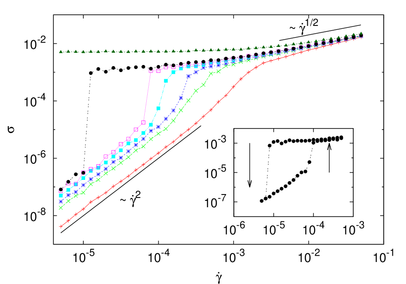
Figure 1: Flow curves $\sigma(\dot{\gamma})$ for different packing fractions $\varphi=0.78,0.7925,0.795,0.7975,0.79875,0.80,0.82$ (from bottom to top). Main part: flow curves obtained by decreasing $\dot{\gamma}$; Inset: example of a hysteresis loop for $\varphi=0.80$.

All the observations can be explained in the framework of a simple model, which can be viewed as a phenomenological Landau theory, that interpolates smoothly between the inertial and the plastic flow regime:

$$\dot{\gamma}(\sigma)=a\sigma^{1/2}-b\sigma+c\sigma^{2},$$ (1)

where $a,b,c$ are coefficients which in general depend on packing fraction. Eq. (1) can be taken to result from a class of constitutive models that combine hydrodynamic conservation laws with a microstructural evolution equation Olmsted (2008), or from mode-coupling approaches Holmes et al. (2005).

The numerical data suggest that the plastic flow regime is only weakly density dependent for packing fractions considered here, so we take $c$ to be independent of $\varphi$ for simplicity. In the inertial flow regime, on the other hand, we expect to see a divergence of the shear viscosity at $\varphi_{\eta}$, implying that the coefficient $a$ of our model vanishes at $\varphi_{\eta}$ and changes sign, $a=a(\varphi)=a_{0}|\varphi_{\eta}-\varphi|(\varphi_{\eta}-\varphi)$. The coefficient $b$ is assumed to be at most weakly density dependent.

The simple model predicts a discontinuous phase transition with a critical point in analogy to the van der Waals theory of the liquid-gas transition (see Fig. 2a). The critical point is determined by locating a vertical inflection point in the flow curve. In other words we require $\partial_{\sigma}\dot{\gamma}=0$ and simultaneously $\partial_{\sigma\sigma}\dot{\gamma}=0$. These two equations together with the constitutive equation (1) determine the critical point: $b_{c}=\frac{3}{2}a(\varphi_{c})^{2/3}c^{1/3}$ with the critical strain rate given by $\dot{\gamma}_{c}=\frac{3}{16}\frac{a^{4/3}}{c^{1/3}}$ and the critical stress $\sigma_{c}=\frac{1}{4}(\frac{a}{c})^{2/3}$. For $\varphi>\varphi_{c}$, the model predicts an unstable region, where $\partial_{\sigma}\dot{\gamma}<0$. This is where the stress jump occurs in the simulations. The flow curves of the model are presented in Fig. 2a, assuming $b\equiv b_{c}$, and fitting the two constants $c,a_{0}$ to the data. The model predicts a yield stress to first occur, when two (positive) zeros for the function $\dot{\gamma}(\sigma)=0$ coincide. This happens at a density $\varphi_{\sigma}$ determined implicitly by $a(\varphi_{c})=a(\varphi_{\sigma})\sqrt{2}$ and the yield stress is given by $\sigma_{yield}=(a/(2c))^{2/3}$. The flow curves can be fitted better, if we allow for weakly density dependent coefficients $b$ and $c$. However, we refrain from such a fit, because even in its simplest form the model can account for all observed features qualitatively: a critical point at $\varphi_{c}$, the appearance of a yield stress at $\varphi_{\sigma}$ and the divergence of the viscosity at $\varphi_{\eta}$, ordered such that $\varphi_{c}<\varphi_{\sigma}<\varphi_{\eta}$. The flow curves for these three packing fractions are highlighted in Fig. 2 and further illustrated in the supplemental material supplement .

The limiting case of frictionless particles can be reached by letting $\mu\to 0$. Simulations indicate that in this limit hysteretic effects vanish Otsuki and Hayakawa (2011, 2009) and the jamming density is increased approaching random close packing. Within the model this transition can be understood in terms of the variation of two parameters: First $b(\mu)\to 0$ in Eq. (1) implies that the three densities $(\varphi_{c},\varphi_{\sigma},\varphi_{\eta})$ coincide and second $\varphi_{\eta}(\mu)\to\varphi_{\rm rcp}\cong 0.8433$. While a $\mu$-dependent $\varphi_{\eta}$ simply shifts the phase diagram towards higher densities, the parameter $b$ accounts for the more important changes of the topology of the phase diagram. The flowcurves in this limit are presented in Fig 2b. They present a continuous jamming scenario consistent with previous simulations in inertial Otsuki and Hayakawa (2009) as well as overdamped systems Olsson and Teitel (2012); Tighe et al. (2010).

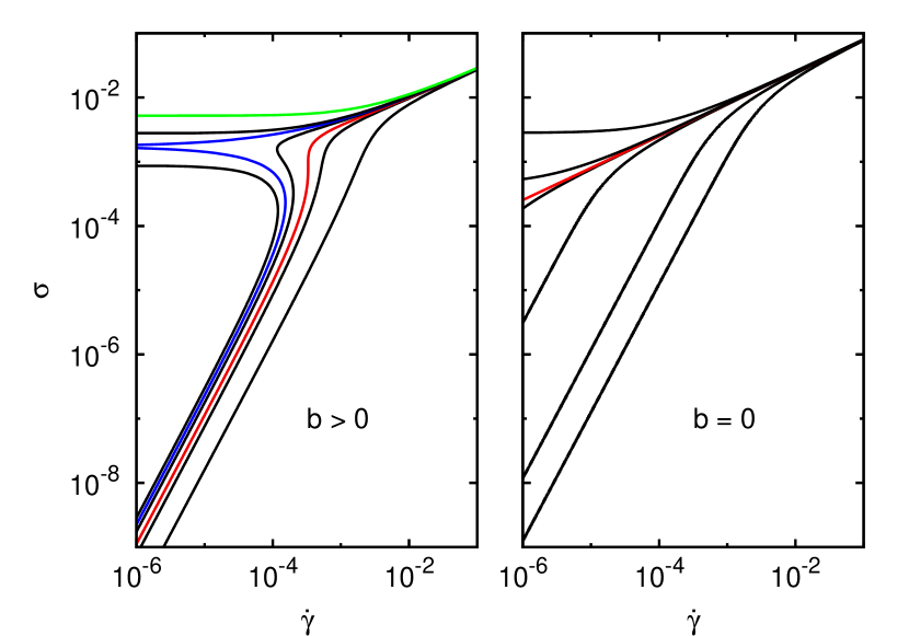
Figure 2: Flow curves of the simple model Eq. (1). Left: Frictional scenario with range of packing fractions as in Fig. 1; $\phi_{c}$ is indicated by the red line, $\phi_{\sigma}$ by the blue line and $\phi_{\eta}$ by the green line. Right: Flow curves for frictionless particles of the simple model implemented with $b=0$ and $\varphi_{c}=\varphi_{\sigma}=\varphi_{\eta}=0.8433$; critical flow curve in red.

What happens in the unstable region? Naively one might expect “coexistence” of the inertial and the plastic flow regime, i.e. shear banding. However, this would have to happen along the vorticity direction Dhont and Briels (2008); Olmsted (2008), which is absent in our two-dimensional setting. Alternative possibilities range from oscillating to chaotic solutions Cates et al. (2002); Nakanishi et al. (2012). We will see that, instead, the system stops flowing and jams at intermediate stress levels. Interestingly, this implies re-entrance in the $(\sigma,\varphi)$ plane with a flowing state both, for large and small stress, and a jammed state in between.

To address the unstable regime in more detail, we have performed stress-controlled simulations: the shear stress is imposed and we measure the strain rate as a function of time. The initial configurations are chosen with a flow profile corresponding to the largest strain rate in the inertial flow regime, which was observed previously in the strain-controlled experiments. For a fixed $\varphi$, several time series are shown in Fig. 3, representing the different regimes. The lowest value of $\sigma_{1}$ is chosen in the inertial flow regime, so that the system continues to flow for large times. Similarly $\sigma_{5}$ is chosen in the plastic flow regime and the system continues to flow as well. The intermediate value $\sigma_{3}$ is chosen in the unstable region and the system immediately jams. Between the jamming and the flow regime we find intermediate phases with transient flow that ultimately stops Ciamarra et al. (2011).

To quantify the different flow regimes, we introduce the time $\tau_{jam}$ the system needs to jam. Schematically we expect the result shown in the lower right corner of Fig. 3: In the jammed phase $\tau_{jam}=0$, whereas in the flow phase $\tau_{jam}$ is infinite. In between $\tau_{jam}$ is finite implying transient flow before the system jams. We expect $\tau_{jam}$ to go to zero as the jammed phase is approached and to diverge as the flow phases are approached. Given that the simulation is run for a finite time, the divergence should be cut off at the time of the simulation run, $T$, indicated by the horizontal (red) line in the schematic in the lower right corner of Fig. 3.

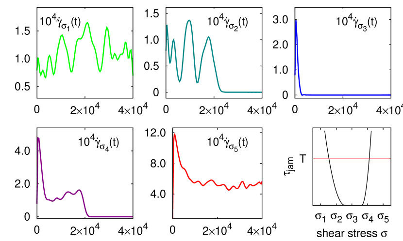
Figure 3: Time series of the strain rate with packing fraction $\varphi=0.7975$ and different, but fixed, stresses $\sigma_{1}<\sigma_{2}<\sigma_{3}<\sigma_{4}<\sigma_{5}$ (stress values are indicated in Fig. 6). Lower right corner: Schematic picture of the jamming time being cut off at the simulation time $T$.

These expectations are borne out by the simulations: In Fig. 4 we show a contour plot of $\tau_{jam}$ as a function of $\varphi$ and $\sigma$. In the dark blue region, $\tau_{jam}$ is very small, corresponding to the jammed state. In the bright yellow region $\tau_{jam}$ exceeds the simulation time; hence this region is identified with the flow regime – inertial flow for small $\sigma$ and plastic flow for large $\sigma$. The intermediate (red) part of the figure corresponds to the transient flow regimes.

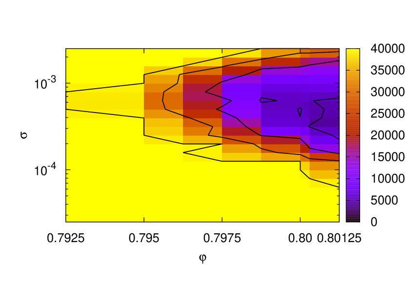
Figure 4: Numerical results for the phase diagram. The mean flow time $\tau_{jam}$ is encoded with color. The flow phase is indicated in yellow (bright) and the jamming phase in blue (dark). Lines are contours of constant $\tau_{jam}$.

In our simple model Eq. (1), the jammed state has to be identified with the unstable region. It seems furthermore suggestive to identify the transient flow regime with metastable regions. The phase diagram, as predicted by the simple model (with finite $b$) is shown in Fig. 5 (schematic). In the region within the (thick) red curve, Eq.(1) has no solution: the system jams. Outside the (thin) blue curve, the solution is unique corresponding to either inertial flow (low stress) or plastic flow (high stress). In between, in the shaded region, the equations allow for two solutions and hence metastable states. Jamming from these metastable states is discontinuous, i.e. the strain rate jumps to zero from a finite value. At a packing fraction $\varphi_{\sigma}$, a yield stress first appears and grows as $\varphi$ is increased further, giving rise to a kink in the red curve and a continuous jamming scenario. Beyond $\varphi_{\eta}$ inertial flow is no longer possible . In the frictionless limit $b\to 0$ all these different packing fractions merge with $\varphi_{\rm rcp}$ giving the phase diagram the simple structure well known from previous work Heussinger and Barrat (2009) and shown in the inset in Fig. 5.

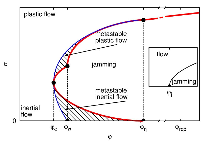
Figure 5: Phase diagram of the model (schematic), revealing re-entrant flow for small and large $\sigma$, as well as flow and jam states in the “metastable” regions for frictional particles (main panel) and the known jamming phase diagram for frictionless particles (inset).

The presence of long transients is fully consistent with the results of Ref. Ciamarra et al. (2011). Due to a restricted stress range in those simulations, however, only the upper part of the phase diagram is captured and the re-entrance behavior is missed. To get a better understanding of these transients (or possibly metastable states), we have tried to construct the flow curves in this regime by the following procedure: The monitored time series are truncated as soon as the system jams. The (transiently) flowing part of the time series is averaged over time, giving rise to the flow curves, shown in Fig. 6. These flow curves show clearly a non-unique relation $\sigma(\dot{\gamma})$ or equivalently a non-monotonic relation $\dot{\gamma}(\sigma)$, which can only be observed as transient behavior, before the system has settled into a stationary state.

Figure 6: Flow curves from the stress-controlled simulations. The unstable branches (decreasing stress) are obtained as time averages over the transient flow (right axis: stress values used for the time series in Fig. 3).

In conclusion: the goal of this paper is to understand the role of friction in the jamming behavior of dry granular matter. To this end we present a theoretical model (supplemented by MD simulations) that can reproduce all the phenomenology of simulated flowcurves (Fig. 2) both for the fully frictional system as well as for the limiting case of frictionless particles. The jamming phase diagrams derived from the model agree with recent experiments Bi et al. (2011). The key result is that the transition between the two jamming scenarios, frictionless/continuous and frictional/discontinuous, can in our model be accounted for by the variation of just a single parameter ($b$). The most important feature of the frictional phase diagram is re-entrant flow and a critical jamming point at finite stress. The fragile “shear jammed” states observed in the experiments Bi et al. (2011) then correspond to the re-entrant (inertial) flow regime in our theory. Our work allows to bring together previously conflicting results Aharonov and Sparks (1999); Chialvo et al. (2012); Ciamarra et al. (2011); Otsuki and Hayakawa (2011) and opens a new path towards a theoretical understanding of a unified jamming transition that encompasses both frictionless as well as frictional particles.