Telegraph Processes with Random Jumps and Complete Market Models

Abstract

We propose a new generalisation of jump-telegraph process with variable velocities and jumps. Amplitude of the jumps and velocity values are random, and they depend on the time spent by the process in the previous state of the underlying Markov process.

This construction is applied to markets modelling. The distribution densities and the moments satisfy some integral equations of the Volterra type. We use them for characterisation of the equivalent risk-neutral measure and for the expression of historical volatility in various settings. The fundamental equation is derived by similar arguments.

Historical volatilities are computed numerically.

Keywords: inhomogeneous jump-telegraph process; dependence on the past; historical volatility; compound Poisson process

Mathematics Subject Classification (2000) 60J27 60J75 60K99 91G99

1 Introduction

The model of non-interacting particles which move with alternating finite velocities was first introduced by [28]. Later, the model was developed by [13] in connection with a certain hyperbolic partial differential equation. In 1956 Mark Kac (see [14]) began to study the telegraph model in detail. Assuming the random time intervals $T_{n}$ between the velocity’s reversal to be independent and exponentially distributed, $T_{n}\sim\mathrm{Exp}(\lambda)$, Kac derived the telegraph (damped wave) equation for the distribution density $p=p(x,t)$ of the particles’ positions,

$$\frac{{\partial}^{2}p}{{\partial}t^{2}}+2\lambda\frac{{\partial}p}{{\partial}t}=c^{2}\frac{{\partial}^{2}p}{{\partial}x^{2}}.$$

Afterwards, the telegraph process and its many generalisations have been studied in great detail. In particular, the generalisations towards motions with the velocities alternated in gamma- or Erlang-distributed random instants have been studied many times, see e. g. [6, 8, 29]. Telegraph processes with random velocities have been considered by [27].

Applications of telegraph processes to market modelling have been presented first by [12], and then, by [20, 10]. Now these applications are transformed into the theory of Markov-modulated market models based on telegraph processes with alternated constant velocities, see e. g. [21, 24] and [17] (see also the survey in [15]). One of the key principles of such a modelling is that the models are based on observable parameters such as velocity and jump amplitude. Replacing the measure, we only change the underlying distributions of time intervals between velocity reversals.

In this paper we assume that the telegraph particle moves with alternated random and variable velocities performing jumps of random amplitude whenever the velocity is changed. The telegraph processes of this type have been studied earlier only under the assumption of mutual independence of velocity values and jump amplitudes, see [27, 17, DiC2013-2]. Here we assume that the actual velocity regime and subsequent jump are determined by the functions of the time spent by the particle in the previous state. We assume also that the time intervals between the state reversals have sufficiently arbitrary distributions. Under these assumptions we obtain the version of telegraph process which possesses some accelerating/damping properties. The paper is a continuation of the paper [25], where such generalisations of the telegraph processes began to be studied. Here the problem is considered in a bit more general setting and with financial applications.

Such a model with deterministic velocities and jumps is studied in detail by [21, 9]. Moreover, earlier we proposed the option pricing model based on jump-telegraph processes, [21]. In this paper we use these processes with random velocity and jumps for the purposes of financial modelling. In particular, this corresponds better to the technical analysis of oversold and overbought markets.

If the random jump amplitudes are statistically independent of the underlying continuous process, then the market model is typically incomplete (see the classical paper by [18], the review by [26] of the jump-diffusion models, and also by [17] for the models based on the telegraph processes).

We profess here the approach of complete markets. In [5] the market model is based on the simple jump process and thus with a single source of randomness. Thus the model is complete. The model, proposed in this paper, typically remains to be complete and arbitrage-free (similar to another simple model with fixed and deterministic jump amplitude [21]). In contrast with [21], in our recent setting the closed formulae for option prices do not exist. To analyse memory properties of the proposed model we numerically evaluate a historical volatility.

The paper is organised as follows. The underlying processes are described in Section 2. Section 3 is devoted to a version of Doob-Meyer decomposition which permits to characterise martingales in our version of jump-telegraph processes. The market model (together with the fundamental equation) is presented in Section 4. We focus on the calculations of historical volatility in Section 5.

2 Generalised jump-telegraph processes

Let $(\Omega,\mathcal{F},{\mathbb{P}})$ be a complete probability space with given filtration $\mathcal{F}_{t},\;t\geq 0$ satisfying the usual hypotheses, [19]. We start with a two-state continuous-time Markov process ${\varepsilon}={\varepsilon}(t)\in\{0,1\},\;t\geq 0$, adapted to $\mathcal{F}_{t}.$ Fixing the initial state of ${\varepsilon}$, consider the conditional probabilities ${\mathbb{P}}_{i},\;i\in\{0,1\}$ with respect to the initial state of ${\varepsilon}$,

$${\mathbb{P}}_{i}(\cdot):={\mathbb{P}}(\cdot~{}|~{}{\varepsilon}(0)=i).$$

The corresponding expectations will be denoted by ${\mathbb{E}}_{i}\{\cdot\}$. Assume that sample paths of ${\varepsilon}={\varepsilon}(t),$ $t\geq 0,$ are right-continuos a. s.

To fix the distribution properties of process ${\varepsilon}$ we begin with the set of independent random variables $T_{n},n\in{\mathbb{Z}},\;T_{n}\geq 0$ with alternated distributions. Denote the respective distribution functions by $F_{0},$ $F_{1},$ the survival functions by $\bar{F}_{0},\;\bar{F}_{1}$ and the densities by $f_{0},\;f_{1}$. The subscript indicates the starting position of the alternation which corresponds to the initial state of ${\varepsilon}$, that is the distribution of $T_{n}$ depends on ${\varepsilon}(0)=i\in\{0,1\}.$ Precisely, under probability ${\mathbb{P}}_{i}$ the distribution function of $T_{n}$ is $F_{i}$, if $n$ is odd, and $F_{1-i}$, if $n$ is even.

Random variables $T_{n}$ are the time intervals between successive switching of Markov process ${\varepsilon}$. Let $\mathfrak{T}=\{\tau_{n}\}$ be the Markov flow of switching times. Then $T_{n}=\tau_{n}-\tau_{n-1}$. We assume the usual non-explosion condition,

$$\tau_{\infty}:=\lim\tau_{n}=+\infty,\qquad{\mathbb{P}}\text{-a.s.}$$

Moreover, let $\tau_{0}=0$, i.e. process ${\varepsilon}$ starts at a switching instant.

The latter assumption can be neglected. If the process is observed beginning from time $s,\;0=\tau_{0}<s<\tau_{1}$, the corresponding conditional distributions can be described by the survival functions

$$\bar{F}_{i}(t~{}|~{}s)= {\mathbb{P}}_{i}(T>t~{}|~{}T>s)=\frac{{\mathbb{P}}_{i}(T>t)}{{\mathbb{P}}_{i}(T>s)}=\frac{\bar{F}_{i}(t)}{\bar{F}_{i}(s)},$$ (2.1)

$$0\leq s<t,\;i=0,1.$$

Therefore, the corresponding densities are

$$f_{i}(t~{}|~{}s)=-\frac{{\partial}}{{\partial}t}\bar{F}_{i}(t~{}|~{}s)=\frac{f_{i}(t)}{\bar{F}_{i}(s)},\quad 0\leq s<t,\quad i=0,1$$

Here $T=T_{1}=\tau_{1}>0$ is the first switching time.

Consider a particle, which moves on ${\mathbb{R}}$ under alternated velocity regimes $c_{0}$ and $c_{1},$ starting from the origin. The velocities are described by two piecewise continuous functions $c_{i}=c_{i}(T,t),\;T,t>0,i=0,1$. At each instant $\tau_{n}\in\mathfrak{T}$ the particle takes the velocity mode $c_{{\varepsilon}(\tau_{n})}(T_{n},\cdot)$, where $T_{n}$ is the (random) time spent by the particle at the previous state before the last switching. We define a generalised telegraph process $\mathcal{T}=\mathcal{T}(t),\;t\geq 0$ driven by the velocity modes $c_{0},\;c_{1}$ as follows,

$$\mathcal{T}(t)=\mathcal{T}(t;c_{0},c_{1})=c_{{\varepsilon}(\tau_{n})}(T_{n},t-\tau_{n}),\quad\text{if~{}~{}}\tau_{n}\leq t<\tau_{n+1},\;n\geq 0.$$ (2.2)

The integral $\int_{0}^{t}\mathcal{T}(s){\rm d}s$ represents the current particle’s position, $\int_{0}^{t}\mathcal{T}(s){\rm d}s$ is named the integrated telegraph process.

Denote by $N=N(t):=\max\{n\geq 0:~{}\tau_{n}\leq t\},\;t\geq 0$ a counting Poisson process. Integrated telegraph processes can be described in terms of the compound Poisson process as follows.

Let $\tau_{n-1}\leq s<t<\tau_{n},\;n\geq 1$. Under the given value $i={\varepsilon}(\tau_{n-1})={\varepsilon}(s)$ denote the distance passed by the particle in time interval $(s,\;t)$ without any reversal by $l_{i}(T;s,t)$,

$$l_{i}(T;s,t)=\int_{s}^{t}c_{i}\left(T,u-\tau_{n-1}\right){\rm d}u.$$ (2.3)

Simplifying notations we will write $l_{i}(T;t)$ instead of $l_{i}(T;0,t)$.

If $N(t)=0$, i. e. $0=\tau_{0}\leq t<\tau_{1}$, and ${\varepsilon}(0)=i$, then the particle’s position is

$$\int\limits_{0}^{t}\mathcal{T}(u){\rm d}u=l_{i}(T_{0};t).$$ (2.4)

If $N(t)>0$, then

$$\int\limits_{0}^{t}\mathcal{T}(u){\rm d}u=\sum_{n=1}^{N(t)}l_{{\varepsilon}(\tau_{n})}(T_{n-1};\tau_{n-1},\tau_{n})+l_{{\varepsilon}(\tau_{N(t)})}(T_{N(t)};\tau_{N(t)},t).$$ (2.5)

Equalities (2.3)-(2.5) define the integrated telegraph process.

Similarly, the jump component can be constructed. Let $h_{0}=h_{0}(T)$ and $h_{1}=h_{1}(T),$ $T\geq 0,$ be a pair of deterministic piecewise continuous (or, at least, boundary measurable) functions. Consider piecewise constant telegraph processes based on $h_{i}(T)$ instead of $c_{i}=c_{i}(T,\cdot),\;i=0,1$, see (2.2):

$$\mathcal{T}(t;h_{0},h_{1})=h_{{\varepsilon}(\tau_{n})}(T_{n}),\quad\text{if~{}~{}}\tau_{n}<t\leq\tau_{n+1},\;n\geq 0.$$

We define an integrated jump process as the compound Poisson process,

$$\int\limits_{0}^{t}\mathcal{T}(u;h_{0},h_{1}){\rm d}N(u)=\sum_{n=1}^{N(t)}h_{{\varepsilon}(\tau_{n})}(T_{n}).$$ (2.6)

The amplitude of the subsequent jump depends on the time spent by the particle in the current state.

Generalised integrated jump-telegraph process is sum of the integrated telegraph process defined by (2.4)-(2.5) and the jump component defined by (2.6):

$$X(t)=\int\limits_{0}^{t}\mathcal{T}(u;c_{0},c_{1}){\rm d}u+\int\limits_{0}^{t}\mathcal{T}(u;h_{0},h_{1}){\rm d}N(u),\quad t\geq 0.$$ (2.7)

We consider also the processes $X_{i},\;i=0,1$, defined by (2.7) under the fixed initial state of ${\varepsilon}(0)=i\in\{0,1\}$. So, $X_{i}(t)$ gives the position at time $t,\;t\geq 0$ of the particle, which starts at the origin with velocity mode $c_{i},\;i={\varepsilon}(0),$ and continues moving with the alternated at random times $\tau_{n}$ velocity regimes. Each velocity reversal is accompanied by jumps of random amplitude.

Conditioning on the first switching, we have the following equalities in distribution (under the probability ${\mathbb{P}}_{0}$ and ${\mathbb{P}}_{1}$ respectively):

$$X_{0}(t)\mid_{{\mathbb{P}}_{0}}\stackrel{{\scriptstyle D}}{{=}}l_{0}(T_{0};t){\bf 1}_{\{\tau_{1}>t\}}+\left[l_{0}(T_{0};\tau_{1})+h_{0}(\tau_{1})+\tilde{X}_{1}(t-\tau_{1})\right]{\bf 1}_{\{\tau_{1}<t\}},$$ (2.8)

where $T_{0}$ and $\tau_{1}$ have the distribution functions $F_{1}$ and $F_{0}$ respectively;

$$X_{1}(t)\mid_{{\mathbb{P}}_{1}}\stackrel{{\scriptstyle D}}{{=}}l_{1}(T_{0};t){\bf 1}_{\{\tau_{1}>t\}}+\left[l_{1}(T_{0};\tau_{1})+h_{1}(\tau_{1})+\tilde{X}_{0}(t-\tau_{1})\right]{\bf 1}_{\{\tau_{1}<t\}},$$ (2.9)

where $T_{0}$ and $\tau_{1}$ are distributed in the opposite order, with distribution functions $F_{0}$ and $F_{1}$ respectively. Here $\tilde{X}_{i}(t)$ is the integrated jump-telegraph process starting with the velocity regime $c_{i}(T_{1};\cdot),\;i=0,1.$

The distributions of $X_{0}(t),X_{1}(t)$ and $X(t),\;t>0,$ are separated into the singular and the absolutely continuous parts. All distributions will be described in terms of the conditional probabilities ${\mathbb{P}}_{i}(\cdot~{}|~{}N(s)=0)$ under the condition $\{N(s)=0\}=\{\tau_{1}>s\}$, see (2.1). Here $s,\;s\in[0,\tau_{1})$ is the time when the observations begin.

For any Borelian set $B\subset(-\infty,\infty)$ consider

$${\mathbb{P}}_{i}(B,t|s):={\mathbb{P}}_{i}(X(t)\in B~{}|~{}N(s)=0),\quad i=0,1.$$

The singular part of the distribution ${\mathbb{P}}_{i}(\cdot,t|s)$ corresponds to the first terms in the RHS of (2.8)-(2.9), the movement without any reversal, $N(t)=0.$ To describe the singular part, consider the linear functionals (generalised functions),

$$\phi\to{\mathbb{P}}_{i}(\tau_{1}>t|N(s)=0){\mathbb{E}}_{i}\{\phi(l_{i}(\tau_{1};t))\}= \bar{F}_{i}(t|s)\int\limits_{0}^{\infty}f_{1-i}(\tau)\phi(l_{i}(\tau;t)){\rm d}\tau,$$

$$i=0,1,$$

on the space of (continuous) test-functions $\phi.$ The generalised function

$$p_{i}^{0}(x,t|s)=\bar{F}_{i}(t|s)\int_{0}^{\infty}f_{1-i}(\tau)\delta_{l_{i}(\tau;t)}(x){\rm d}\tau,\quad i=0,1$$ (2.10)

can be viewed as the (conditional) distribution “density”. Here $\delta_{a}(x)$ is the Dirac measure (of unit mass) at point $a$.

Let

$$p_{i}(x,t|s)={\mathbb{P}}_{i}\left(X(t)\in{\rm d}x~{}|~{}N(s)=0\right)/{\rm d}x$$

be the distribution densities of $X_{i}(t),\;i=0,1$.

By conditioning on the first velocity reversal we obtain the following system of integral equations

$$p_{0}(x,t|s)= p_{0}^{0}(x,t|s)$$ (2.11)

$$+ \int_{0}^{\infty}f_{1}(\tau){\rm d}\tau\int_{s}^{t}p_{1}(x-l_{0}(\tau;u)-h_{0}(u),t-u)f_{0}(u|s){\rm d}u,$$

$$p_{1}(x,t|s)= p_{1}^{0}(x,t|s)$$

$$+ \int_{0}^{\infty}f_{0}(\tau){\rm d}\tau\int_{s}^{t}p_{0}(x-l_{1}(\tau;u)-h_{1}(u),t-u)f_{1}(u|s){\rm d}u,$$

$$t>s\geq 0,\;x\in(-\infty,\infty),$$

where $p_{i}^{0},\;i=0,1,$ are defined by (2.10).

Then, systems similar to (2.11) can be derived for the expectations.

Let $\mu_{i}(t|s):={\mathbb{E}}_{i}\{X(t)~{}|~{}N(s)=0\},\;t>s\geq 0$ be the conditional expectation with respect to ${\mathbb{P}}_{i}(\cdot|N(s)=0),$ and $\mu_{i}(t):={\mathbb{E}}_{i}\{X(t)\}=\lim\limits_{s\downarrow 0}\mu_{i}(t|s),$ $i=0,1$.

One can easily obtain, for $t>s$

$$\mu_{i}(t|s)=\bar{F}_{i}(t|s)\bar{l}_{i}(t)+\int_{s}^{t}\left(\bar{l}_{i}(u)+h_{i}(u)+\mu_{1-i}(t-u)\right)f_{i}(u|s){\rm d}u,$$

where $\bar{l}_{i}(\cdot)={\mathbb{E}}\{l_{i}(T;\cdot)\}=\int_{0}^{\infty}f_{1-i}(\tau)l_{i}(\tau;\cdot){\rm d}\tau,\;i=0,1$.

Therefore, the conditional expectations $\mu_{0}(t|s)$ and $\mu_{1}(t|s)$ read as,

$$\mu_{0}(t|s)= a_{0}(t|s)+\int_{s}^{t}\mu_{1}(t-u)f_{0}(u|s){\rm d}u,$$ (2.12)

$$\mu_{1}(t|s)= a_{1}(t|s)+\int_{s}^{t}\mu_{0}(t-u)f_{1}(u|s){\rm d}u.$$

Hence, the expectations $\mu_{i}=\mu_{i}(t)={\mathbb{E}}_{i}\{X(t)\},\;i=0,1$ satisfy the following Volterra-type system

$$\mu_{0}(t)= a_{0}(t)+\int_{0}^{t}\mu_{1}(t-u)f_{0}(u){\rm d}u,$$ (2.13)

$$\mu_{1}(t)= a_{1}(t)+\int_{0}^{t}\mu_{0}(t-u)f_{1}(u){\rm d}u.$$

Here

$$a_{i}(t|s):=\bar{F}_{i}(t|s)\bar{l}_{i}(t)+\int_{s}^{t}(\bar{l}_{i}(u)+h_{i}(u))f_{i}(u|s){\rm d}u,\quad t>s,$$

and $a_{i}(t)=a_{i}(t|0),\;i=0,1.$ Integrating by parts in the latter integral, we have

$$\int_{s}^{t}\bar{l}_{i}(u)f_{i}(u|s){\rm d}u=-\bar{F}_{i}(t|s)\bar{l}_{i}(t)+\bar{l}_{i}(s)+\int_{s}^{t}\bar{c}_{i}(u)\bar{F}_{i}(u|s){\rm d}u,$$

which leads to the following expression for $a_{i}(t|s)$:

$$a_{i}(t|s)=\bar{l}_{i}(s)+\int_{s}^{t}\left(\bar{F}_{i}(u|s)\bar{c}_{i}(u)+f_{i}(u|s)h_{i}(u)\right){\rm d}u.$$

Since $\bar{l}_{i}(0)=0$ and $\bar{F}_{i}(t|0)=\bar{F}_{i}(t),\;f_{i}(t|0)=f_{i}(t)$, we get

$$a_{i}(t)=\int_{0}^{t}\left(\bar{F}_{i}(u)\bar{c}_{i}(u)+f_{i}(u)h_{i}(u)\right){\rm d}u.$$ (2.14)

Moreover, the equalities in (2.1) and (2.14) lead to

$$a_{i}(t|s)= \bar{l}_{i}(s)+\bar{F}_{i}(s)^{-1}\int_{s}^{t}\left(\bar{F}_{i}(u)\bar{c}_{i}(u)+f_{i}(u)h_{i}(u)\right){\rm d}u$$ (2.15)

$$= \bar{l}_{i}(s)+\bar{F}_{i}(s)^{-1}\left(a_{i}(t)-a_{i}(s)\right),\quad i=0,1.$$

Here we denote $\bar{c}_{i}(s)={\mathbb{E}}\{c_{i}(\cdot;s)\}=\int_{0}^{\infty}f_{1-i}(\tau)c_{i}(\tau;s){\rm d}\tau$.

Remark 2.1.

The Volterra system (2.13) has a unique solution, see e. g. [16]. Moreover, $\mu_{0}(t)\equiv 0$, $\mu_{1}(t)\equiv 0$ if and only if $a_{0}(t)\equiv 0,a_{1}(t)\equiv 0$, or equivalently,

$$\begin{aligned} \bar{F}_{0}(t)\bar{c}_{0}(t)+h_{0}(t)f_{0}(t)=0\\ \bar{F}_{1}(t)\bar{c}_{1}(t)+h_{1}(t)f_{1}(t)=0\end{aligned}\;,\qquad t\geq 0,$$ (2.16)

see (2.14).

Hence, $\mu_{0}(t)\equiv 0$, $\mu_{1}(t)\equiv 0$ if and only if the hazard rate functions of the spending time $T,\;T>0,$ see e.g. [3],

$$\alpha_{i}(t):=\frac{f_{i}(t)}{\bar{F}_{i}(t)}$$ (2.17)

are expressed by $\alpha_{i}(t)=-\bar{c}_{i}(t)/h_{i}(t),\;t\geq 0.$

Due to equations (2.12) and (2.14)-(2.15), condition (2.16) guarantees that

$$\mu_{0}(t|s)=\bar{l}_{0}(s),\qquad\mu_{1}(t|s)=\bar{l}_{1}(s).$$ (2.18)

In some particular cases the solution of (2.12) and (2.13) can be written explicitly. Consider the following example. Let the alternated distributions of interarrival times are exponential:

$$f_{i}(t)=\lambda_{i}\exp(-\lambda_{i}t),\quad t\geq 0,\;i=0,1.$$ (2.19)

Hence $f_{i}(t|s)=\lambda_{i}\exp(-\lambda_{i}(t-s)),\;t>s\geq 0.$ In this case the solution of system (2.13) reads

$$\boldsymbol{\mu}(t)=\boldsymbol{a}(t)+\int_{0}^{t}\left(I+\varphi_{\lambda}(t-u)\Lambda\right)L\boldsymbol{a}(u){\rm d}u,$$ (2.20)

where

$$\varphi_{\lambda}(t)=\frac{1-{\rm e}^{-2\lambda t}}{2\lambda},\quad 2\lambda:=\lambda_{0}+\lambda_{1}.$$ (2.21)

Here we use the matrix notations $\boldsymbol{\mu}=(\mu_{0},\mu_{1})^{\prime},$ $\boldsymbol{a}=(a_{0},a_{1})^{\prime}$, see (2.14),

$$L=\begin{pmatrix}0&\lambda_{0}\\ \lambda_{1}&0\end{pmatrix}\qquad\text{and}\qquad\Lambda=\begin{pmatrix}-\lambda_{0}&\lambda_{0}\\ \lambda_{1}&-\lambda_{1}\end{pmatrix}.$$

To check it, notice that system (2.13) is equivalent to ODE with zero initial condition:

$$\frac{{\rm d}\boldsymbol{\mu}(t)}{{\rm d}t}=\Lambda\boldsymbol{\mu}(t)+\boldsymbol{\psi}(t),\quad t>0,\qquad\boldsymbol{\mu}(t)\mid_{t\downarrow 0}=\boldsymbol{0},$$

where $\boldsymbol{\psi}=\dfrac{{\rm d}\boldsymbol{a}}{{\rm d}t}+(L-\Lambda)\boldsymbol{a}.$ We obtain this equation differentiating in (2.13) with subsequent integration by parts. Clearly, the equation is solved by

$$\boldsymbol{\mu}(t)=\int_{0}^{t}{\rm e}^{(t-u)\Lambda}\boldsymbol{\psi}(u){\rm d}u.$$ (2.22)

Integrating by parts in (2.22) we obtain

$$\boldsymbol{\mu}(t)=\boldsymbol{a}(t)+\int_{0}^{t}{\rm e}^{(t-u)\Lambda}L\boldsymbol{a}(u){\rm d}u.$$

Since $\Lambda^{2}=-2\lambda\Lambda$, the exponential of $t\Lambda$ is

$$\exp\{t\Lambda\}={\rm I}+\varphi_{\lambda}(t)\Lambda=\frac{1}{2\lambda}\begin{pmatrix}\lambda_{1}+\lambda_{0}{\rm e}^{-2\lambda t}&\quad\lambda_{0}(1-{\rm e}^{-2\lambda t})\\ \\ \lambda_{1}(1-{\rm e}^{-2\lambda t})&\quad\lambda_{0}+\lambda_{1}{\rm e}^{-2\lambda t}\end{pmatrix},$$

and then, we have (2.20).

The explicit formulae for conditional expectations $\mu_{i}(t|s),\;i=0,1$ follow directly from (2.12) and (2.20).

Equations for variances $\sigma_{i}(t):=\mathrm{Var}\{X_{i}(t)\}={\mathbb{E}}\{\left(X_{i}(t)-\mu_{i}(t)\right)^{2}\},\;t>0,$ have the form, similar to (2.13):

$$\sigma_{0}(t)= b_{0}(t)+\int_{0}^{t}\sigma_{1}(t-u)f_{0}(u){\rm d}u,$$ (2.23)

$$\sigma_{1}(t)= b_{1}(t)+\int_{0}^{t}\sigma_{0}(t-u)f_{1}(u){\rm d}u,$$

where

$$b_{i}(t):= \bar{F}_{i}(t)\left(\bar{l}_{i}(t)-\mu_{i}(t)\right)^{2}$$

$$+ \int_{0}^{t}\left(\bar{l}_{i}(u)+h_{i}(u)+\mu_{1-i}(t-u)-\mu_{i}(t)\right)^{2}f_{i}(u){\rm d}u,\quad i=0,1.$$

In the special case of exponential distributions (2.19) the solution of (2.23) reads similar to (2.20).

More specifically, the solution of (2.23) is given by

$$\boldsymbol{\sigma}=\boldsymbol{b}(t)+\int_{0}^{t}(I+\varphi_{\lambda}(t-u)\Lambda)L\boldsymbol{b}(u){\rm d}u,$$ (2.24)

where $\boldsymbol{\sigma}=(\sigma_{0},\sigma_{1})^{\prime},\;\boldsymbol{b}=(b_{0},b_{1})^{\prime}$. We use also the notations of (2.20) and (2.21).

Remark 2.2.

Let $0=\tau_{0}<\tau_{1}<\tau_{2}<\ldots$ be a Poisson univariate point process with deterministic constant intensity $2\lambda,\;\lambda>0$. Let $Y_{n},n\geq 1$ be a sequence of the i. i. d. random variables with two values, $Y_{n}\in\{0,1\}$. We may then consider two counting processes

$$N^{(0)}(t):=\sum_{n\geq 1}{\bf 1}_{\{\tau_{n}\leq t\}}{\bf 1}_{\{Y_{n}=0\}},\quad N^{(1)}(t):=\sum_{n\geq 1}{\bf 1}_{\{\tau_{n}\leq t\}}{\bf 1}_{\{Y_{n}=1\}}.$$

It is easy to see that $N^{(i)}(t),\;t\geq 0$ is a univariate point process with intensity $\lambda_{i},\;i=0,1.$ Here $\lambda_{0}=2\lambda(1-p)$ and $\lambda_{1}=2\lambda p,$ where $p={\mathbb{P}}(Y_{n}=1).$ In the special case (2.19) the Markov flow $\mathfrak{T}$ is the bivariate point process $(N^{(0)}(t),N^{(1)}(t))$. See [2].

3 Martingales

Let $X=X(t)$ be integrated jump-telegraph process defined by (2.7) on the filtered probability space $(\Omega,\mathcal{F},\{\mathcal{F}_{t}\}_{t\geq 0},{\mathbb{P}})$.

Theorem 3.1.

Process $X$ is $\mathcal{F}_{t}$-martingale if and only if (2.16) holds.

Proof.

We need to show that (2.16) is necessary and sufficient for

$${\mathbb{E}}\left\{X(t)~{}|~{}\mathcal{F}_{s}\right\}=X(s),\quad 0<s<t.$$ (3.1)

First, notice that for any stopping times $t$ and $s$ such that, $s<t$, we have

$${\mathbb{E}}_{i}\{X(t)-X(s)~{}|~{}{\mathcal{F}}_{s}\}={\mathbb{E}}_{i}\left\{\int_{s}^{t}\mathcal{T}(u;c_{0},c_{1}){\rm d}u+\sum_{k=N(s)+1}^{N(t)}h_{{\varepsilon}(\tau_{k})}(T_{k})~{}|~{}{\mathcal{F}}_{s}\right\}$$

$$={\mathbb{E}}_{i}\left\{\int_{0}^{t-s}\mathcal{T}(s+u){\rm d}u+\sum_{k=1}^{N(t)-N(s)}h_{{\varepsilon}(\tau_{k+N(s)})}(T_{k+N(s)})~{}|~{}{\mathcal{F}}_{s}\right\}$$

on the set $0\leq s\leq t$.

Let $s,\;s\geq 0$ be a switching time, $s=\tau_{n}$ (in this case the proof is similar to [25]). According to the Markov property by definition of the processes ${\varepsilon}={\varepsilon}(t),\;N=N(t)$ and $\tau_{k}$ we have the following identities in (conditional) distribution

$${\varepsilon}(\tau_{n}+u)|_{\{{\varepsilon}(\tau_{n})=i\}}\stackrel{{\scriptstyle D}}{{=}} \tilde{\varepsilon}(u)|_{\{\tilde{\varepsilon}(0)=i\}},\quad u\geq 0,$$

$$N(t)|_{\{{\varepsilon}(\tau_{n})=i\}}\stackrel{{\scriptstyle D}}{{=}} n+\tilde{N}(t-\tau_{n})|_{\{\tilde{\varepsilon}(0)=i\}},\quad t\geq\tau_{n}\geq 0,$$

$$\tau_{k+n}|_{\{{\varepsilon}(\tau_{n})=i\}}\stackrel{{\scriptstyle D}}{{=}} \tilde{\tau}_{k}|_{\{\tilde{\varepsilon}(0)=i\}},\;T_{k+n}|_{\{{\varepsilon}(\tau_{n})=i\}}\stackrel{{\scriptstyle D}}{{=}}\tilde{T}_{k}|_{\{\tilde{\varepsilon}(0)=i\}}, \quad k\geq 0,$$

where $\tilde{\varepsilon}(s),\;\tilde{N}(s),\;\tilde{\tau}_{k}$ and $\tilde{T}_{k}$ are copies of ${\varepsilon}(s),\;N(s),\;\tau_{k}$ and $T_{k}$ respectively, independent of $\mathcal{F}_{\tau_{n}}$. Hence, we obtain

$${\mathbb{E}}\{X(t)-X(\tau_{n})~{}|~{}{\mathcal{F}}_{\tau_{n}}\}={\mathbb{E}}_{i}\{\tilde{X}(t-\tau_{n})\},$$

if ${\varepsilon}(\tau_{n})=i$. Here $\tilde{X}$ denotes the integrated jump-telegraph process, which is based on $\tilde{\varepsilon},\;\tilde{N},\;\tilde{\tau}_{k}$ and $\tilde{T}_{k}$, starting from the state $\tilde{\varepsilon}(0)=i$. The latter expectation is equal to zero, ${\mathbb{E}}_{i}\{\tilde{X}(t-\tau_{n})\}\equiv 0$, if and only if (2.16) holds. Thus, equality (3.1) is proved, if $s$ is the switching time, $s=\tau_{n}$.

In general, for any $s,\;s<t$ the martingale property (3.1) is proved by using (2.18), Remark 2.1. ∎

Remark 3.1.

Notice that if $X$ is the martingale, so identities (2.16) hold, then the direction of each jump should be opposite to the respective (mean) velocity value.

Remark 3.2.

In the special case of process $X$ with exponential distributions of interarrival times (2.19) the set of equalities (2.16) is equivalent to

$$\bar{c}_{0}(t)+\lambda_{0}h_{0}(t)=0,\qquad\bar{c}_{1}(t)+\lambda_{1}h_{1}(t)=0,$$

see also Theorem 1 in [21].

Theorem 3.2.

Let the jump-telegraph process $X$ be defined by (2.7), and $h_{i}\neq 0,$ $i=0,1$. If $X$ is the martingale, then

$$\frac{\bar{c}_{i}(t)}{h_{i}(t)}< 0\qquad\forall t>0,$$ (3.2)

$$\int_{0}^{\infty}\frac{\bar{c}_{i}(s)}{h_{i}(s)}{\rm d}s= -\infty,\quad i=0,1.$$ (3.3)

Moreover, $X$ is the martingale, if and only if the the hazard rate functions $\alpha_{i}(t)$ ( see the definition in (2.17)) of interarrival times are expressed by

$$\alpha_{i}(t)=-\bar{c}_{i}(t)/h_{i}(t),\;t\geq 0.$$ (3.4)

Therefore, the distribution densities of interarrival times satisfy the following set of integral equations:

$$f_{i}(t)=\alpha_{i}(t)\exp\left\{-\int_{0}^{t}\alpha_{i}(s){\rm d}s\right\}\equiv-\frac{\bar{c}_{i}(t)}{h_{i}(t)}\exp\left\{\int_{0}^{t}\frac{\bar{c}_{i}(s)}{h_{i}(s)}{\rm d}s\right\},\qquad t>0,\;i=0,1.$$ (3.5)

Proof.

Equations (3.4) are derived, see Theorem 3.1. By these equations

$$-\frac{\bar{c}_{i}(t)}{h_{i}(t)}=\alpha_{i}(t)=\frac{f_{i}(t)}{\bar{F}_{i}(t)}\equiv-(\ln\bar{F}_{i}(t))^{\prime},\quad t\geq 0,\;i=0,1.$$ (3.6)

Thus the survival probability is

$$\bar{F}_{i}(t)=\exp\left\{\int_{0}^{t}\frac{\bar{c}_{i}(s)}{h_{i}(s)}{\rm d}s\right\},\qquad t\geq 0,\;i=0,1.$$

So, the density is given by (3.5).

Inequality (3.2) follows from (2.16). Notice that by definition $\lim\limits_{t\to+\infty}\bar{F}_{i}(t)=0,$ hence (3.3) is valid.∎

Consider the following example. Assume that functions $\bar{c}_{i}(t)$ and $h_{i}(t)$ are proportional:

$$\frac{\bar{c}_{i}(t)}{h_{i}(t)}\equiv-\lambda_{i},\qquad\lambda_{i}>0,\;i=0,1.$$ (3.7)

Therefore, by (3.5) the respective integrated jump-telegraph process is the martingale if the distributions of interarrival times are exponential with densities $f_{i}(t)=\lambda_{i}\exp(-\lambda_{i}t),$ $t>0,\;i=0,1.$

Identities (3.7) can be written in detail as follows. Let $X$ be the jump-telegraph process with regimes of velocities $c_{0},c_{1}$ and the regimes of jumps $h_{0},h_{1}$, which are connected by means of the relations

$$\lambda_{1}\int_{0}^{\infty}{\rm e}^{-\lambda_{1}\tau}c_{0}(\tau,t){\rm d}\tau=-\lambda_{0}h_{0}(t),\qquad\lambda_{0}\int_{0}^{\infty}{\rm e}^{-\lambda_{0}\tau}c_{1}(\tau,t){\rm d}\tau=-\lambda_{1}h_{1}(t).$$

Here $\lambda_{0}$ and $\lambda_{1}$ are some positive constants. Hence the jump-telegraph process $X$ is the martingale with exponentially distributed interarrival times. Parameters of these alternated exponential distributions are $\lambda_{0}$ and $\lambda_{1}$.

Equations (3.7) permit to interpret the switching intensities $\lambda_{0}$ and $\lambda_{1}$ by using the (observable) proportion between velocity and jump values. On the other hand, if the average velocity regimes are given, $\bar{c}_{0}$ and $\bar{c}_{1}$, and $X_{0}$ and $X_{1}$ are martingales, then we can observe the details of comportment of process $X=X(t)$. For example, the martingale possesses small jumps with high frequency, while the big jumps are rare. The direction of jump should be opposite to the velocity sign, see also Remark 3.1.

Other useful examples are presented in [25], see Examples 1-4, pp.2289-2290.

Proposition 3.1.

Let $\mathfrak{T}=\{\tau_{n}\}$ be the Markov flow of switching times, and $X$ be a jump-telegraph process defined by (2.7). Suppose that the increments $T_{n}=\tau_{n}-\tau_{n-1},\;n\geq 1$ are exponentially distributed with alternated parameters $\mu_{0},\mu_{1}>0$.

Assume that the velocity regimes $c_{i}=c_{i}(T,t)$ and the jump amplitudes $h_{i}=h_{i}(t)$ are proportional satisfying (3.7) with some positive coefficients $\lambda_{0}$ and $\lambda_{1}$.

Therefore the martingale measure for $X$ exists and it is unique. Under the martingale measure the interarrival times are exponential with parameters $\lambda_{0}$ and $\lambda_{1}$.

Proof.

For the integrated jump-telegraph process defined by (2.7) we define the Radon-Nikodym derivative of the form, see [21]

$$\frac{{\rm d}{\mathbb{Q}}}{{\rm d}{\mathbb{P}}}=\exp\left\{\int_{0}^{t}\mathcal{T}(u;c_{0}^{*},c_{1}^{*}){\rm d}u\right\}\kappa^{*}(t).$$ (3.8)

Here $X^{*}=X^{*}(t)$ is the jump-telegraph process driven by the Markov flow $\mathfrak{T}$ (with parameters $\mu_{0}>0$ and $\mu_{1}>0$). Process $X^{*}$ is defined by the constant velocities $c_{0}^{*}=\mu_{0}-\lambda_{0}$ and $c_{1}^{*}=\mu_{1}-\lambda_{1}$ and the constant jump parameters $h_{0}^{*}=-c_{0}^{*}/\mu_{0},\;h_{1}^{*}=-c_{1}^{*}/\mu_{1}.$ The jump part $\kappa^{*}(t)=\prod_{n=1}^{N(t)}(1+h_{{\varepsilon}(\tau_{n-1})}^{*})$ follows from the exponential formula, [26], and $\int_{0}^{t}\mathcal{T}(u;c_{0}^{*},c_{1}^{*}){\rm d}u$ is the integrated telegraph process.

Since Theorem 2 and Theorem 3 in [21], under the new measure ${\mathbb{Q}}$ the underlying Markov flow takes the intensities $\lambda_{i}$ instead of $\mu_{i},\;i=0,1$, see also [4] (Lemma1) and [26] (Theorem 2.5).

Since, due to (3.7), condition (2.16) is fulfilled. By Theorem 3.2 the process $X(t)$ becomes the ${\mathbb{Q}}$-martingale. ∎

4 Market model and fundamental equation

Let the price process $S=S(t)$ be defined by stochastic exponential of generalised jump-telegraph process $X$. The velocity and jump regimes are established in accordance with time spent by the process in the previous state (see the definition in (2.7)).

Precisely, let ${\varepsilon}={\varepsilon}(t)\in\{0,1\},\;t\in[0,U]$ be the Markov process describing the evolution of market states. Let $\mathfrak{T}=\{\tau_{n}\}$ be the flow of switching times. Consider the integrated jump-telegraph process $X=X(t)$ based on ${\varepsilon}$ and $\mathfrak{T}$, which is defined by (2.7) with velocity regimes $c_{0}=c_{0}(T,t),\;c_{1}=c_{1}(T,t)$ and jump amplitudes $h_{0}(T),\;h_{1}(T)>-1,\;\forall T\geq 0$.

Consider a market model of one risky asset associated with price process $S=S(t)$, which is the stochastic exponential,

$$S(t)=S(0)\mathcal{E}_{t}\{X\}=S(0)\exp\left\{\int_{0}^{t}\mathcal{T}(s;c_{0},c_{1}){\rm d}s\right\}\kappa(t),\quad t\in[0,U].$$ (4.1)

Here $\kappa(t)=\prod_{n=1}^{N(t)}(1+h_{{\varepsilon}(\tau_{n-1})}(T_{n}))$ is the jump component of stochastic exponential $\mathcal{E}_{t}\{X\}$, see the exponential formula of Stieltjes-Lebesgue calculus ([2], Theorem T4 in Appendix A4; see also [26], formula (17)).

Let $r_{0}=r_{0}(T,t)\geq 0,\;r_{1}=r_{1}(T,t)\geq 0,\;T,t\geq 0$ be piecewise continuous deterministic functions. The bond price is assumed to be

$$B(t)=\exp\left\{\int_{0}^{t}\mathcal{T}(u;r_{0},r_{1}){\rm d}u\right\}.$$ (4.2)

Here $\mathcal{T}(\cdot;r_{0},r_{1})$ is the telegraph process driven by the same Markov process ${\varepsilon}$ (see (2.2)) and $r_{0},\;r_{1}$ are the interest rate functions. Thus, the discounted price process is of the same structure as $S(t)$, (4.1),

$$B(t)^{-1}S(t)=S(0)\exp\left\{\int_{0}^{t}\mathcal{T}(u;c_{0}-r_{0},c_{1}-r_{1}){\rm d}u\right\}\kappa(t).$$

Hence, without loss of generality we assume the interest rates to be 0.

Let ${\mathbb{Q}}$ be the martingale measure for process $S$, (4.1).

Consider an option with the payoff function $\mathcal{H}=\mathcal{H}(x),\;\mathcal{H}(x)\geq 0$ at the maturity time $U,\;U>0$.

Let $A_{i}(t|s,{\rm d}s):=\{{\varepsilon}(t)=i,\;t-\tau_{N(t)}\in(s,s+{\rm d}s)\},t\in(0,U),$ $i=0,1.$ Here $s\in(0,t),$ and $\tau_{N(t)}$ is the last switching time. Notice that $A_{i}(t|s,{\rm d}s)\in\mathcal{F}_{t}.$ Consider the functions

$$\Phi_{i}(x,t|s,{\rm d}s)= {\mathbb{E}}_{\mathbb{Q}}\left\{\mathcal{H}(x{\rm e}^{\int_{t}^{U}\mathcal{T}(u;c_{0},c_{1}){\rm d}u}\kappa(U)/\kappa(t))~{}|~{}A_{i}(t|s,{\rm d}s)\right\}{\mathbb{Q}}(A_{i}(t|s,{\rm d}s))$$

$$= \int\limits_{A_{i}(t|s,{\rm d}s)}\mathcal{H}(x{\rm e}^{\int_{t}^{U}\mathcal{T}(u;c_{0},c_{1}){\rm d}u}\kappa(U)/\kappa(t)){\rm d}{\mathbb{Q}},$$

$$0\leq s<t\leq U,\;i=0,1,$$

see (2.1). Further, let $\Phi_{i}(x,t|s)=\lim\limits_{{\rm d}s\downarrow 0}\Phi_{i}(x,t|s,{\rm d}s).$

Notice that the strategy value at time $t\in(0,U)$ equals to

$$V(t|s)=\Phi_{{\varepsilon}(t)}(S(t),t|s),$$

where $s=t-\tau_{N(t)}$ is the elapsed time since the last switching.

Conditioning on the first reversal after time $t$, we see the explicit expressions for functions $\Phi_{0}(x,t|s)$ and $\Phi_{1}(x,t|s)$,

$$\Phi_{0}(x,t|s)= \bar{F}_{0}(U-t+s){\mathbb{E}}\left\{\mathcal{H}(x{\rm e}^{l_{0}(\tau;t,U)})\right\}$$ (4.3)

$$+ {\mathbb{E}}\left\{\int_{t}^{U}f_{0}(u-t+s)\mathrm{\Phi}_{1}(x{\rm e}^{l_{0}(\tau;t,u)}(1+h_{0}(u-t+s)),u){\rm d}u\right\},$$

$$\Phi_{1}(x,t|s)= \bar{F}_{1}(U-t+s){\mathbb{E}}\left\{\mathcal{H}(x{\rm e}^{l_{1}(\tau;t,U)})\right\}$$

$$+ {\mathbb{E}}\left\{\int_{t}^{U}f_{1}(u-t+s)\mathrm{\Phi}_{0}(x{\rm e}^{l_{1}(\tau;t,u)}(1+h_{1}(u-t+s)),u){\rm d}u\right\}.$$

Here $\mathrm{\Phi}_{0}(\cdot,t)$ and $\mathrm{\Phi}_{1}(\cdot,t)$ are defined by $\mathrm{\Phi}_{i}(x,t)=\lim\limits_{s\downarrow 0}\Phi_{i}(x,t|s),\;i=0,1$. Functions $\mathrm{\Phi}_{i}(\cdot,t),\;i=0,1$ correspond to the market process initiated exactly at the switching time.

Finally, notice that functions $\mathrm{\Phi}_{0}(\cdot,t)$ and $\mathrm{\Phi}_{1}(\cdot,t)$ solve the following Volterra system:

$$\mathrm{\Phi}_{0}(x,t)= \bar{F}_{0}(U-t){\mathbb{E}}\left\{\mathcal{H}(x{\rm e}^{l_{0}(\tau;t,U)}\right\}$$ (4.4)

$$+ {\mathbb{E}}\left\{\int_{t}^{U}f_{0}(u-t)\mathrm{\Phi}_{1}(x{\rm e}^{l_{0}(\tau;t,u)}(1+h_{1}(u-t)),u){\rm d}u\right\},$$

$$\mathrm{\Phi}_{1}(x,t)= \bar{F}_{1}(U-t){\mathbb{E}}\left\{\mathcal{H}(x{\rm e}^{l_{1}(\tau;t,U)}\right\}$$

$$+ {\mathbb{E}}\left\{\int_{t}^{U}f_{1}(u-t)\mathrm{\Phi}_{0}(x{\rm e}^{l_{1}(\tau;t,u)}(1+h_{0}(u-t)),u){\rm d}u\right\}.$$

The set of integral equations (4.3)-(4.4) can be interpreted as the fundamental equation of the market model (4.1)-(4.2). In the case of deterministic and constant velocities and jumps these equations are equivalent to a hyperbolic PDE-system, see equation (36) in [21].

Remark 4.1.

Consider the model (4.1)-(4.2) with constant $c_{i},h_{i}$ and $r_{i},\;i=0,1$ in the special case of exponentially distributed iterarrival times, (2.19). The fundamental equations (4.3)-(4.4) take the form of PDE-system:

$$\frac{\partial\mathrm{\Phi}_{i}}{\partial t}(t,x)+c_{i}x\frac{\partial\mathrm{\Phi}_{i}}{\partial x}(t,x) =(r_{i}+\lambda_{i})\mathrm{\Phi}_{i}(t,x)-\lambda_{i}\mathrm{\Phi}_{1-i}(t,x(1+h_{i})),$$ (4.5)

$$0<t<T,\quad i=0,\;1.$$

Equation (4.5) is supplied with the terminal condition

$$\mathrm{\Phi}_{i}(x,\;T)=\mathcal{H}(x).$$ (4.6)

5 Memory effects. Numerical results

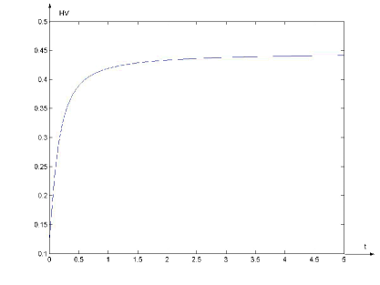
Figure 1: Historical volatility under the constant velocities and jump amplitudes (symmetric case): $c_{0}=1,\;h_{0}=-0.05;\;$ $c_{1}=-1,\;h_{1}=0.05;\;$ $\lambda_{0}=\lambda_{1}=5$

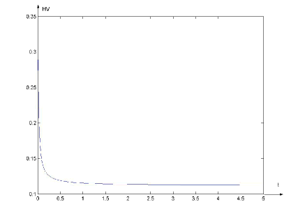
Figure 2: Historical volatility under the constant velocities and jump amplitudes (symmetric case): $c_{0}=1,\;h_{0}=-0.05;\;$ $c_{1}=-1,\;h_{1}=0.05;\;$ $\lambda_{0}=\lambda_{1}=80$

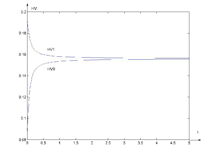
Figure 3: Historical volatility under the constant velocities and jump amplitudes: $c_{0}=1.2,\;h_{0}=-0.05;\;$ $c_{1}=0.6,\;h_{1}=-0.02;\;$ $\lambda_{0}=\lambda_{1}=15$

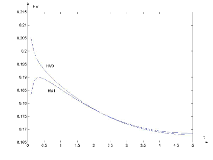
Figure 4: Historical volatility under the constant velocities and jump amplitudes: $c_{0}=1.2,\;h_{0}=-0.05;\;$ $c_{1}=0.6,\;h_{1}=-0.02;\;$ $\lambda_{0}=24,\lambda_{1}=30$

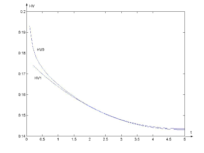
Figure 5: Historical volatility under the variable velocities and jump amplitudes: $c_{0}(t)=\frac{1.2}{1+1.2t},\;h_{0}=\frac{-0.05}{1+1.2t};\;$ $c_{1}=\frac{0.6}{1+0.6t},\;h_{1}=\frac{-0.02}{1+0.6t};\;\;$ $\lambda_{0}=24,\lambda_{1}=30$.

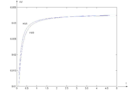
Figure 6: Historical volatility under the variable velocities and jump amplitudes: $c_{0}(t)=-0.5t,\;h_{0}=0.02t;\;$ $c_{1}=-t,\;h_{1}=0.05t;\;$ $\lambda_{0}=25,\lambda_{1}=20$.

We demonstrate the memory effects related to the jump-telegraph model by means of the historical volatility ${\rm H\negthickspace V}(\cdot)$ defined by

$${\rm H\negthickspace V}(t):=\sqrt{\frac{{\rm Var}\{\log S(t)\}}{t}}.$$ (5.1)

For the Black-Scholes model the historical volatility is constant, ${\rm H\negthickspace V}(t)\equiv\sigma$.

The models that capture the memory effects of the market, possess a variable historical volatility. Consider a moving-average type model, which is described by the log-price

$$\log S(t)/S(0)= at+\sigma w(t)-\sigma\int_{0}^{t}{\rm d}\tau\int_{-\infty}^{\tau}\lambda_{0}{\rm e}^{-(\lambda_{0}+\lambda_{1})(\tau-u)}{\rm d}w(u),$$

$$\sigma,\;\lambda_{1},\;\lambda_{0}+\lambda_{1}>0,$$

see [1]. This model is specially designed for the description of exponentially decaying memory. The historical volatility is exactly described by

$${\rm H\negthickspace V}(t)=\frac{\sigma}{\lambda_{0}+\lambda_{1}}\sqrt{\lambda_{1}^{2}+\lambda_{0}(2\lambda_{1}+\lambda_{0})\varphi_{\lambda}(t)/t},$$ (5.2)

where $\varphi_{\lambda}$ is defined by (2.21). See formula (4.8) in [1].

Consider the market model, based on the stochastic exponential of jump-telegraph process $X=X(t),\;t\in[0,U]$, see (4.1). Surprisingly, the historical volatility of this model agrees with the models of a moving-average type, see [1]. For convenience, we define the historical volatility in jump-telegraph model by ${\rm H\negthickspace V}_{i}(t):=\sqrt{\sigma_{i}(t)/t},\;i=0,1$ instead of (5.1). Here $\sigma_{0}(t)={\rm Var}\{X_{0}(t)\}$ and $\sigma_{1}(t)={\rm Var}\{X_{1}(t)\}$ solve system (2.23). The explicit formulae for ${\rm H\negthickspace V}_{i}(t)$ are rather cumbersome, even if the case of constant and deterministic velocities and jumps. Nevertheless, it is easy to compute the limits of ${\rm H\negthickspace V}_{i}(t)$ as $t\to 0$ and as $t\to\infty$:

$$\lim\limits_{t\to 0}{\rm H\negthickspace V}_{i}(t) =\sqrt{\lambda_{i}}|h_{i}|,$$

$$\lim\limits_{t\to\infty}{\rm H\negthickspace V}_{i}(t) =\sqrt{\frac{\lambda_{0}\lambda_{1}}{2\lambda^{3}}\left[(\lambda_{0}B+c)^{2}+(\lambda_{1}B-c)^{2}\right]},\quad i=0,1,$$

see (4.5)-(4.6) in [22]. Here the jump-telegraph process $X$ is defined with the constant velocities $c_{0},c_{1},\;c_{0}>c_{1}$ and with the constant jumps $h_{0},\;h_{1}>-1$; $\lambda=(\lambda_{0}+\lambda_{1})/2,\;B=(h_{0}+h_{1})/2$ and $c=(c_{0}-c_{1})/2$; the subscript $i={\varepsilon}(0)$ indicates the initial market state.

In the symmetric case, $\lambda_{0}=\lambda_{1}=\lambda$, the historical volatility ${\rm H\negthickspace V}_{i}(t),\;t\geq 0$ can be expressed by

$${\rm H\negthickspace V}_{i}(t)= \sqrt{\frac{c^{2}}{\lambda}+\lambda B^{2}+(c+\lambda b)^{2}\frac{\varphi_{2\lambda}(t)}{\lambda t}+\gamma_{i}\frac{\varphi_{\lambda}(t)}{t}+(-1)^{i}2B(c+\lambda b){\rm e}^{-2\lambda t}},$$ (5.3)

$$i=0,\;1,$$

where $b=(h_{0}-h_{1})/2,\gamma_{i}=-2c(c/\lambda+(-1)^{i}h_{i}),\;i=0,1,$ see formula (4.2) in [22].

In particular, if in this symmetric case the jumps are also symmetric, $h_{0}=-h_{1}=h,$ and $X$ is the martingale, $c+\lambda h=0$, then $B=0,\;c+\lambda b=0$ and $\gamma_{0}=\gamma_{1}=0$. So (5.3) gives the constant historical volatility, ${\rm H\negthickspace V}_{0}={\rm H\negthickspace V}_{1}\equiv c/\sqrt{\lambda}.$ In general, formula (5.3) comports with formulae for historical volatility of the history dependent model with memory (5.2).

Fig. 1-2 contain the plots in the symmetric case. Here ${\rm H\negthickspace V}_{0}\equiv{\rm H\negthickspace V}_{1}$. Fig. 3-4 also represent the model with constant parameters. In these cases we use directly formula (5.3).

Some other computations and plots of historical and implied volatilities with constant parameters $c_{i},h_{i},i=0,1,$ see also in [23].

We compute the historical volatility for the variable (deterministic) velocities and jumps as the solution of system (2.23) by formula (2.24). Fig. 5 and Fig. 6 show the result.

References

- [1] Anh V, Inoue A (2005) Financial markets with memory I: dynamic models. Stoch Anal Appl 23:275-300
- [2] Brémaud P (1981) Point processes and queues: martingale dynamics, Springer Verlag, New York
- [3] Capasso V, Bakstein D (2005) An Introduction to Continuous-Time Stochastic Processes. Birkhäuser, Boston, Basel, Berlin
- [4] Cheang GHL, Chiarella C (2011) A modern view on Merton s jump-diffusion model. Research paper. University of Technology Sydney, Quantitative Finance Research Centre
- [5] Cox JC, Ross SA (1976) The valuation of options for alternative stochastic processes. J Fin Econ 3:145-166
- [6] Di Crescenzo A (2001) On random motions with vetocities alternating at Erlang-distributed random times. Adv Appl Prob 33:690-701
- [7] i Crescenco A, Iuliano A, Martinucci B, Zacks S (2013) Generalized telegraph process with random jumps. J Appl Prob 50:450-463
- [8] Di Crescenzo A, Martinucci B (2010) A damped telegraph random process with logistic stationary distribution. J Appl Prob 47:84-96
- [9] Di Crescenzo A, Martinucci B (2013) On the generalized telegraph process with deterministic jumps. Methodol Comput Appl Prob 15:215-235
- [10] Di Crescenzo A, Pellerey F (2002) On prices’ evolutions based on geometric telegrapher’s process. Appl Stoch Models Bus Ind 18:171-184
- [11] Föllmer H, Protter P (2011) Local martingales and filtration shrinkage. ESAIM: Probab Stat 15:S25-S38. doi: 10.1051/ps/2010023
- [12] Di Masi G, Kabanov Y, Runggaldier W (1994) Mean-variance hedging of options on stocks with Markov volatilities. Theory Probab Appl 39:172-182
- [13] Goldstein S (1951) On diffusion by discontinuous movements and on the telegraph equation. Quart J Mech Appl Math 4:129-156
- [14] Kac M (1974) A stochastic model related to the telegrapher s equation. Rocky Mountain J Math 4:497-509. Reprinted from: M. Kac, Some stochastic problems in physics and mathematics, Colloquium lectures in the pure and applied sciences, No. 2, hectographed, Field Research Laboratory, Socony Mobil Oil Company, Dallas, TX, 1956, pp. 102-122.
- [15] Kolesnik AD, Ratanov N (2013) Telegraph Processes and Option Pricing. Springer, Heidelberg
- [16] Linz P (1985) Analytical and Numerical Methods for Volterra Equations. SIAM, Philadelphia
- [17] López O, Ratanov N (2012) Option pricing under jump-telegraph model with random jumps. J Appl Prob 49:838-849
- [18] Merton RC (1976) Option pricing when underlying stock returns are discontinuous. J Financial Economics 3:125-144
- [19] Protter P (2005) Stochastic Integration and Differential Equations. Version 2.1. Springer-Verlag, Heidelberg
- [20] Ratanov N (1999) Telegraph processes and option pricing, 2nd Nordic-Russian Symposium on Stochastic Analysis, Beitostolen, Norway.
- [21] Ratanov N (2007a) A jump telegraph model for option pricing. Quantitative Finance 7:575-583
- [22] Ratanov N (2007b) Jump telegraph processes and financial markets with memory. J Appl Math Stoch Anal. doi:10.1155/2007/72326
- [23] Ratanov N (2008) Jump telegraph processes and a volatility smile. Math Meth Econ Fin 3:93-111
- [24] Ratanov N (2010) Option pricing model based on a Markov-modulated diffusion with jumps. Braz J Prob Stat 24:413-431
- [25] Ratanov N(2013) Damped jump-telegraph processes. Stat Prob Lett 83: 2282-2290
- [26] Runggaldier WJ (2003) Jump diffusion models. In : Handbook of Heavy Tailed Distributions in Finance (S.T. Rachev, ed.), Handbooks in Finance, Book 1 (W.Ziemba Series Ed.), Elesevier/North-Holland, pp.169-209
- [27] Stadje W, Zacks S (2004) Telegraph processes with random velocities. J Appl Prob 41:665-678
- [28] Taylor GI (1922) Diffusion by continuous movements. Proc Lond Math Soc 20:196-212
- [29] Zacks S (2004) Generalized integrated telegraph processes and the distribution of related stopping times. J Appl Prob 41:497-507