Rogue waves in nonlinear Schrödinger models with variable coefficients: application to Bose-Einstein condensates

Abstract.

We explore the form of rogue wave solutions in a select set of case examples of nonlinear Schrödinger equations with variable coefficients. We focus on systems with constant dispersion, and present three different models that describe atomic Bose-Einstein condensates in different experimentally relevant settings. For these models, we identify exact rogue wave solutions. Our analytical findings are corroborated by direct numerical integration of the original equations, performed by two different schemes. Very good agreement between numerical results and analytical predictions for the emergence of the rogue waves is identified. Additionally, the nontrivial fate of small numerically induced perturbations to the exact rogue wave solutions is also discussed.

Keywords: Rogue wave, Variable coefficient Nonlinear Schrödinger equation, BEC

PACS numbers: 02.30.Ik,03.75.Lm,42.65.Tg

1. Introduction

Extreme wave events, initially reported in ocean seafarer stories and later observed by satellite surveillances [1], have become a subject of increased interest in physical oceanography [2]. In this context, pertinent water waves are known as rogue waves (alias “freak” or “extreme” waves), and are tentatively defined as waves whose height is more than twice the significant wave height, which is itself defined as the averaged of the highest third of the waves in a time series [2]; therefore, rogue waves are large waves for a given sea state. The conditions that cause rogue waves to grow enormously in size are not fully understood up to now, although there exists an ongoing effort (see, e.g., Refs. [3, 4]) and discussions [5] regarding this problem.

Obviously, the elucidation of the mechanisms underlying the formation and dynamics of rogue waves is a subject of fundamental scientific interest; as such, it has attracted significant attention not only in the more standard ocean-surface-dynamical problem [2], but also in other physical contexts. Indeed, there exists a vast amount of theoretical work in various fields ranging from optics (see, e.g., the recent work [6, 7, 8, 9, 10] and references therein) and atomic Bose-Einstein condensates (BECs) [11], to plasmas [12], laser-plasma interactions [13], atmospheric dynamics [14], and even econophysics [15]; see also the recent short review of [16, 17].

In addition, many experimental observations of rogue waves have been reported in different settings, including nonlinear optics [18, 19, 20], mode-locked lasers [21], superfluid helium [22], hydrodynamics [23], Faraday surface ripples [24], parametrically driven capillary waves [25], and plasmas [26].

Interestingly enough, in many of the above contexts, the models that are used to describe rogue waves are variants of a universal nonlinear evolution equation, namely the nonlinear Schrödinger (NLS) equation. The latter is ubiquitous in wave packet propagation in nonlinear dispersive media, describing, e.g., the amplitude of deep water waves, the electric field envelope in optical media, the macroscopic wave function in superfluids, etc. Importantly, rogue wave events may be triggered by instabilities (e.g., the modulational instability [27]) that are present in NLS models. On the other hand, the NLS equation itself supports solutions that reproduce the qualitative characteristics of rogue waves to a highly satisfactory extent: indeed, earlier pioneering works by Peregrine [28], Kuznetsov [29], Ma [30], and Akhmediev [31] (and also the work of Dysthe and Trulsen [32]), succeeded in constructing rogue-wave-like rational solutions of the NLS model. Importantly, the relevance of this analytical toolbox for rogue waves, was later established in various experiments carried out in different physical contexts (see, e.g., Refs. [19, 23, 26]).

In this work, we study rogue wave solutions in NLS models with variable coefficients. Such models have gained attention, mainly due to their relevance in different physical contexts and, especially, in atomic Bose-Einstein condensates (BECs) [33, 34] and nonlinear optics [35]. In particular, in the physics of BECs, an NLS [alias Gross-Pitaevskii (GP)] equation usually incorporates an external spatially-dependent potential, which can also become time-dependent [33]; additionally, the nonlinearity coefficient (which is proportional to the $s$-wave scattering length) may vary in time or/and in space by employing external magnetic [36] or optical [37] fields close to Feshbach resonances. On the other hand, in the context of optics, NLS equations with varying dispersion have been studied in the context of dispersion managed systems [38]; furthermore, in nonlinear optical systems, the transverse (to the propagation direction) refractive index profile appears as a spatially-dependent potential term –similar to that in BECs– while modulation of the nonlinearity coefficient is possible too (see, e.g., the review [39] and references therein). Localized solutions and solitons of NLS models with variable coefficients have been studied in many works, while connection of such models with integrable ones has been investigated as well (see, e.g., [40, 41, 42, 43, 44, 45, 46, 47] and references therein). Notice that “nonautonomous rogons”, namely rogue waves in a variable coefficient NLS model, were also studied recently [48].

Here, we consider a fairly general $(1+1)$-dimensional NLS model, incorporating an external potential (thus resembling the GP equation in BECs); the latter, along with the dispersion and nonlinearity coefficients are assumed to be functions of both independent variables. Then, following the analysis of Ref. [45], we obtain exact rogue wave solutions of the considered NLS model by using a general transformation for the unknown field, which involves a “seed solution” that satisfies the usual NLS model, expressed in appropriate new variables. The latter, along with auxiliary amplitude and phase functions involved in the transformation of the unknown field, depend on a set of auxiliary functions and parameters. Focusing on the case of constant dispersion, we show that proper choices of these auxiliary functions and parameters, lead to three specific models, which can be used to describe atomic BECs in different, yet experimentally tractable, settings. For these models, which have not been presented or studied before (to the best of our knowledge) in the context of rogue waves, exact analytical rogue wave solutions are presented. Our analytical results are corroborated by direct numerical simulations, that are performed in the original NLS model, and have been based on two different integration schemes. For each of the three models, we find very good agreement between the two schemes, as well as with the analytically predicted form of each rogue wave solution. However, these computations raise a number of nontrivial concerns about the robustness of these solutions. In particular, we will see that in most of the considered cases, for times beyond the formation of the Peregrine soliton (which will represent a rogue wave in our case examples), spontaneously a modulational instability of the background emerges that produces an expanding sequence of bright solitary waves in the system. We will thus also briefly discuss the relevant observations in light of the particular form of our numerical computations (and the examination of two distinct high order numerical schemes).

The paper is structured as follows. In Section 2 we introduce our model, the analytical methodology, as well as the rogue wave solutions; we also present and discuss the above mentioned three specific models that find application in the physics of BECs, as well as their rogue wave solutions. Section 3 is devoted to a detailed numerical study of these three models, and to a comparison between our numerical methods and analytical predictions. Finally, Section 4 presents our conclusions.

2. Analytical considerations

2.1. Model and outline of the analytical method

We start from a generic $(1+1)$-dimensional NLS equation with variable coefficients, which is expressed in dimensionless form as follows:

$$i\frac{\partial\psi}{\partial t}+\frac{D}{2}\frac{\partial^{2}\psi}{\partial x^{2}}-g|\psi|^{2}\psi-V\psi=0,$$ (1)

where $\psi(x,t)$ is a complex field, which represents the macroscopic wave function in BECs or the electric field envelope in optics; note that in the latter context, $t$ denotes propagation distance, and $x$ represents either retarded time (for pulses in optical fibers) or transverse spatial coordinate (for beams in waveguides) [35]. Furthermore, $D$ and $g$ denote the dispersion and nonlinearity coefficients, while $V$ is an external potential; the latter denotes the trap confining the atoms in BECs [33], or the linear part of the transverse refractive index profile in optics [35]. Here, we will consider the case $D=D(x,t)$, $g=g(x,t)$ and $V=V(x,t)$, i.e., the dispersion and nonlinearity coefficients, as well as the external potential, are real functions of $x$ and $t$.

Variants of Eq. (1) have been studied in Refs. [40, 41, 42], in the contexts of quasi one-dimensional (1D) BECs and nonlinear optical systems. Particularly, in the case of BECs, the external trap $V$ is naturally spatially inhomogeneous and can also become time-dependent by using time-varying magnetic or optical fields [33], while the inhomogeneity in $g$ (i.e., in the inter-atomic collision dynamics) can be induced by means of the Feshbach-resonance management technique; this relies on a direct control of the $s$-wave scattering length in BECs by employing external (temporally and/or spatially) varying magnetic [36] or optical [37] fields close to Feshbach resonances. On the other hand, in the case of optical systems, $V$ and $g$ (i.e., the linear and nonlinear parts of the refractive index) may be varying in artificial setups, such as the light-induced photonic lattices [52] or the structure composed by layers of silica alternating with empty gaps [53]. Furthermore, the dispersion coefficient $D$ may also vary, e.g., in the case of dispersion-managed optical fiber systems and lasers [38].

Following the analysis of Ref. [45], we introduce the transformation:

$$\psi(x,t)=q(X,T)p(x,t)\exp[i\phi(x,t)],$$ (2)

and reduce Eq. (1) to the usual nonlinear Schrödinger equation satisfied by the auxiliary field $q=q(X,T)$:

$$i\frac{\partial q}{\partial T}+\frac{1}{2}\frac{\partial^{2}q}{\partial X^{2}}+s|q|^{2}q=0,$$ (3)

where $s=\pm 1$. The new variable $X=X(x,t)$, along with the field $p=p(x,t)$ and the phase $\phi=\phi(x,t)$, as well as $D$, $g$ and $V$, are determined explicitly by means of a set of arbitrary functions $f_{1}(t)$, $f_{2}(t)$, $f_{3}(t)$, $T(t)$, and $F(x)$, with a simple condition $F(x)f_{1}(t)>0$ (see [45] and also our specific examples below). By choosing the above arbitrary functions, the dispersion and nonlinearity coefficients $D$ and $g$, as well as the potential $V$ in Eq. (1), can be “designed” and analytically determined. Therefore, solutions of Eq. (1) can be found by means of solutions of the standard NLS of Eq. (3). Here, as we will show below, using the transformation of Eq. (2) and a rogue wave solution of Eq. (3), we can determine rogue wave solutions of the original model of Eq. (1).

2.2. Rogue waves for systems with constant dispersion

We now focus on NLS systems with constant dispersion $D$, which are relevant to the context of atomic BECs. Based on the results of Ref. [45], $D={\rm const.}$ can be achieved by choosing $F(x)=c_{1}$. In such a case, the new variables $X(x,t)$ and $T(t)$, the field $p(x,t)$ and phase $\phi(x,t)$, as well as the dispersion, nonlinearity and potential functions $D$, $g$ and $V$ of Eq. (1), are given in terms of three real arbitrary functions, $f_{1}(t)$, $f_{2}(t)$ and $f_{3}(t)$, and three real constants, $c_{1}$, $c_{2}$ and $c_{3}$ (under the condition $c_{1}f_{1}(t)>0$), as follows:

$$X(x,t)=c_{1}f_{1}(t)x+f_{3}(t),\quad T(t)=c_{2}\int f_{1}^{2}(t)dt+c_{3},$$ (4)

$$p(x,t)=\sqrt{\frac{f_{1}(t)}{c_{1}}},\quad\phi(x,t)=-\dfrac{c_{1}}{2c_{2}}\frac{c_{1}\dot{f}_{1}(t)x^{2}+2\dot{f}_{3}(t)x}{f_{1}(t)}+f_{2}(t),$$ (5)

$$D=\dfrac{c_{2}}{c_{1}^{2}}={\rm const.},\quad g=-sc_{2}c_{1}f_{1}(t),\quad V(x,t)=v_{2}x^{2}+v_{1}x+v_{0},$$ (6)

where dots denote derivatives with respect to $t$, and the coefficients $v_{k}$ $(k=0,1,2)$ appearing in the expression of the potential $V(x,t)$ are given by:

$$v_{2} = -\frac{c_{1}^{2}}{2c_{2}}\frac{2\dot{f}_{1}^{2}(t)-f_{1}(t)\ddot{f}_{1}(t)}{f_{1}^{2}(t)},$$ (7)

$$v_{1} = -\frac{c_{1}}{c_{2}}\frac{2\dot{f}_{1}(t)\dot{f}_{3}(t)-f_{1}(t)\ddot{f}_{3}(t)}{f_{1}^{2}(t)},$$ (8)

$$v_{0} = -\frac{1}{2c_{2}}\frac{2c_{2}f_{1}^{2}(t)\dot{f}_{2}(t)+\dot{f}_{3}^{2}(t)}{f_{1}^{2}(t)}.$$ (9)

We now assume that the seed solution $q(X,T)$ of the transformation (2) is a rogue wave solution of the NLS Eq. (3); here, we consider the Peregrine soliton, which has the form (see, e.g., Ref. [4]):

$$q(X,T)=\left[1-\frac{{4(1+2iT)}}{{1+4{T^{2}}+4{X^{2}}}}\right]\exp(iT).$$ (10)

Then, the respective solution $\psi(x,t)$ of Eq. (1) is given by:

$$\psi(x,t) = \sqrt{\frac{f_{1}(t)}{c_{1}}}\left[1-\frac{4\left(1+2i(c_{2}\int f_{1}^{2}(t)dt+c_{3})\right)}{1+4\left(c_{2}\int f_{1}^{2}(t)dt+c_{3}\right)^{2}+4\left(c_{1}f_{1}(t)x+f_{3}(t)\right)^{2}}\right]$$ (11)

$$\times \exp\left[i\left(c_{2}\int f_{1}^{2}(t)dt-\frac{c_{1}}{2c_{2}}\frac{c_{1}\dot{f}_{1}(t)x^{2}+2\dot{f}_{3}(t)x}{f_{1}(t)}+f_{2}(t)+c_{3}\right)\right].$$

It is clear that if $f_{1}(t)$ [and, thus, the field $p(x,t)$] is a bounded function of $t$, then Eq. (11) describes a rogue wave solution of Eq. (1). Notice that still other rogue wave solutions can be found, upon choosing the seed solution $q$ to be, e.g., the second-order rogue wave of Ref. [4], the Kuznetsov-Ma soliton [29, 30], the Akhmediev breather [31, 32], and so on.

Notice that our approach for deriving rogue wave solutions of Eq. (1) is, arguably, simpler as compared, e.g., with the methodology of Ref. [40], that involves the solution of a complicated Riccati equation for the coefficients of the NLS, which is not solvable in general.

2.3. Specific models and their rogue wave solutions

Having described our analytical approach, we now proceed by presenting three specific case examples, namely three particular versions of Eq. (1) and their rogue wave solutions. Here, we will present the analytical results for these cases, while the next section will be devoted to the corresponding direct numerical simulations.

2.3.1. Rogue wave on a periodic background.

Our first case example corresponds to the choice: $f_{1}(t)=2+\sin(t)$, $f_{2}(t)=f_{3}(t)=1$, and $c_{1}=c_{2}=c_{3}=1$. In this case, for $s=+1$ in Eq. (3), we find that the field $p$ is given by $p=\sqrt{2+\sin(t)}$, while the coefficients of Eq. (1) are: $D=1$, $g=-(2+\sin(t))$, and $V=-[\big{(}2\cos^{2}(t)+2\sin(t)+\sin^{2}(t)\big{)}x^{2}][2(2+\sin(t))^{2}]^{-1}$. In other words, Eq. (1) takes the form:

$$i\dfrac{\partial\psi}{\partial t}+\dfrac{1}{2}\dfrac{\partial^{2}\psi}{\partial x^{2}}+[2+\sin(t)]|\psi|^{2}\psi=\dfrac{1}{2}\Omega^{2}(t)x^{2}\psi,$$ (12)

$$\Omega^{2}(t)=-\dfrac{2\cos^{2}(t)+2\sin(t)+\sin^{2}(t)}{(2+\sin(t))^{2}}.$$ (13)

Physically speaking, this equation models a BEC, with a scattering length (i.e., nonlinearity coefficient) being periodically modulated in time; this can be achieved by using a periodic external magnetic or optical field near a Feshbach resonance [36, 37], as mentioned above. Notice that since the nonlinearity coefficient is always positive in the context of Eq. (12), the interatomic interactions are always attractive (as in the case of ⁷Li [49, 50] or ⁸⁵Rb [51] atoms). Furthermore, the external potential $V$ is characterized by a normalized frequency $\Omega$ which is also time-periodic, and can either be confining, when the relevant prefactor $\Omega^{2}(t)>0$, or expulsive, for $\Omega^{2}(t)<0$ (note that such an expulsive potential was used in the experiment of Ref. [50]).

In the case under consideration, it is straightforward to find the specific form of the rogue wave solution, using Eq. (11). Since its functional form is rather complicated, we opt not to show it here. Instead, it is quite useful to illustrate the density (square modulus) $|\psi|^{2}$ of this solution, which is shown in Fig. 1. It is clearly observed that the rogue wave exists on a periodic background (left panel), and is characterized by a sharp peak followed by density depressions (right panel).

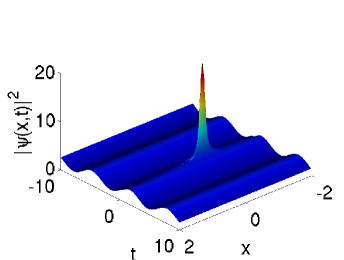
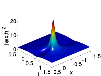
Figure 1. The density profile of the rogue wave with a periodic background. The left panel shows both the background and the rogue wave, while the right panel shows in more detail the local profile of the rogue wave.

2.3.2. Rogue wave on a monotonically decreasing background.

We now consider the following choice of the arbitrary functions and parameters: $f_{1}(t)=\exp(-t)$, $f_{2}(t)=f_{3}(t)=0$, and $c_{1}=c_{3}=1$, $c_{2}=2$. Then, for a focusing nonlinearity ($s=+1$) in Eq. (3), we find that the field $p$ is given by $p=\exp(-t/2)$, while the coefficients of Eq. (1) are: $D=2$, $g=-2\exp(-t)$, and $V=-x^{2}/4$. Thus, Eq. (1) now becomes:

$$i\dfrac{\partial\psi}{\partial t}+\dfrac{\partial^{2}\psi}{\partial x^{2}}+2e^{-t}|\psi|^{2}\psi+\dfrac{1}{4}x^{2}\psi=0.$$ (14)

The above model may describe the dynamics of an attractive BEC (composed by ⁷Li [49, 50] or ⁸⁵Rb [51] atoms), under the action of a purely expulsive potential, described by the last term in the left-hand side of Eq. (14). The scattering length (i.e., the nonlinearity coefficient) is again time-dependent –and this can be achieved by time-varying magnetic [36] or optical [37] fields close to Feshbach resonance. In this case, the magnitude of the scattering length assumes an exponentially decreasing in time form, which can be realized by a ramp down of the applied external fields (such a ramp down of magnetic fields was used in the experiments of Refs. [49, 50]).

As before, the profile of the rogue wave solution for the above mentioned choice can be found analytically by substituting the relevant functions and parameters in Eq. (11). In this case, it is easy to find the density $|\psi|^{2}$ of the rogue wave, which is given by:

$$|\psi{|^{2}}=\dfrac{e^{-t}(65e^{8t}+8e^{6t}x^{2}+16e^{4t}x^{4}+32x^{2}e^{2t}-64e^{4t}x^{2}-144e^{6t}+136e^{4t}+16-64e^{2t})}{(5e^{4t}+4x^{2}e^{2t}+4-8e^{2t})^{2}}.$$ (15)

It is clear that this rogue wave exists on top of a monotonically decreasing background, as imposed by the form of the field $p$ (recall that $p=\exp(-t/2)$ in this case). The density profile of the rogue wave on top of this background, along with a focused snapshot showing its local profile in more detail, are respectively shown in the left and right panels of Fig. 2.

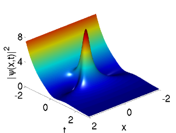
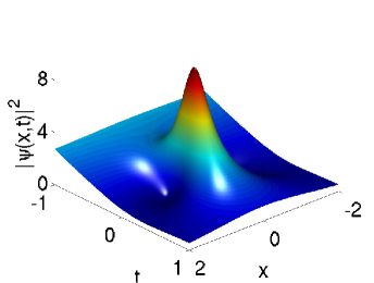
Figure 2. The density profile of the rogue wave with a monotonically decreasing background. The left panel shows both the background and the rogue wave, while the right panel shows in more detail the local profile of the rogue wave.

2.3.3. Twisted rogue wave on a constant background.

Our last case example, corresponds to the following choice: $f_{1}(t)=1$, $f_{2}(t)=-(1/12)[3\cos(t)\sin(t)+3t]$, $f_{3}(t)=-\sin(t)$, and $c_{1}=c_{2}=1$, $c_{3}=0$; then, for a focusing nonlinearity in Eq. (3) (i.e., for $s=+1$), we find that the field $p$ is constant, $p=1$, while the dispersion, nonlinearity and potential in Eq. (1) are respectively given by: $D=1$, $g=-1$, and $V=x\sin(t)$. Thus, Eq. (1) becomes:

$$i\dfrac{\partial\psi}{\partial t}+\dfrac{1}{2}\dfrac{\partial^{2}\psi}{\partial x^{2}}+|\psi|^{2}\psi-x\sin(t)\psi=0.$$ (16)

The above equation is actually a Gross-Pitaevskii model, describing the dynamics of a BEC with attractive interactions (e.g., a ⁷Li [49, 50] or a ⁸⁵Rb [51] BEC), which evolves in a linear (in space) potential, whose amplitude is sinusoidally modulated in time. In earlier BEC experiments, such a linear potential was actually realized by a gravitational one [54], while in more recent experiments with BECs loaded in optical lattices, linear potentials periodically modulated in time were also implemented by using laser beams [55]. It should also be noted that theoretical studies on non-autonomous BEC solitons in such time-dependent linear potentials have been reported as well [56].

Let us now proceed with the presentation of the rogue wave solution of Eq. (16), which has the form:

$$\psi=-\dfrac{3-4x^{2}+8x\sin(t)-4\sin^{2}(t)-4t^{2}+8it}{1+4x^{2}-8x\sin(t)+4\sin^{2}(t)+4t^{2}}e^{-(i/4)[-4x\cos(t)+\cos(t)\sin(t)-3t]}.$$ (17)

Notice that since $p=1$ in this case, the background of this rogue wave is constant. In fact, it is found that the density profile of the above solution bears many similarities with the one of the NLS equation [cf. Eq. (10)]; nevertheless, the orientation of the rogue wave is different in this case, as can be seen by a “twist” about the origin $(0,0)$ in the $(x-t)$ plane –cf. Fig. 3. For this reason, hereafter, the rogue wave of Eq. (17) will be called “twisted rogue wave”.

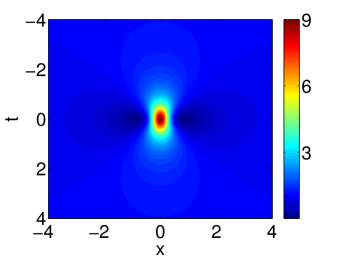
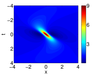
Figure 3. Contour plots showing the density profiles of the rogue wave solution of the NLS equation (left panel) and the rogue wave solution of Eq. (16) (right panel). Observe the relative “twist” of the latter about the origin $(0,0)$ in the $(x-t)$ plane.

3. Numerical Results

3.1. Numerical methods.

In this section, we present results of direct numerical integration of Eq. (1). While our analysis above indicates the existence of exact solutions of Eq. (1), the time evolution dynamics is used to explore the robustness of these explicit solutions under the numerically induced perturbations (due not only to roundoff error, but also due to the local truncation error arising by spatially and temporally discretizing the dynamics). Our numerical scheme is briefly described in what follows.

Initially, the second-order partial derivatives with respect to $x$ are replaced by second-order central differences on a grid consisting of $N$ equidistant points of the form $x_{j}=-L+2jL/(N+1)$ with $j=1,\dots,N$ and $\Delta x=2L/(N+1)$, where $L$ determines the size of the spatial domain. In what follows, the grid size and its resolution are chosen and fixed to be $L=300$ and $\Delta x=0.05$, respectively (although, structurally, our results were not especially sensitive to the particular choices). As regards boundary conditions, we note that we use no-flux conditions at the edges of the spatial grid, namely $\partial_{x}\psi(x,t)|_{x=-L}=\partial_{x}\psi(x,t)|_{x=L}=0$. The latter are replaced by forward and backward first-order finite difference formulas, respectively.

As far as the time integration is concerned, the Dormand and Prince (DOP853) method with an automatic time-step procedure [57] is employed to solve the underlying system of nonlinear ODEs. However, the standard 4th-order Runge-Kutta (RK4) method with a fixed time-step is employed as well, and used to compare its results with the ones found using the former method. Throughout the subsequent presentation, and for the RK4 method in particular, the time step-size ranges from $\Delta t=10^{-4}$ to $\Delta t=10^{-6}$ depending on the particular case studied. Finally, the initialization of the dynamics is performed using the rogue wave solution of Eq. (11), adjusted to the models studied in the previous section. Notice that since in the expression of Eq. (11), the rogue wave arises around $t=0$, the numerical integration is initialized shortly before $t=0$, namely at a slightly negative time, in order to observe the rogue wave formation, as it arises in our modified NLS models.

3.2. Results of the simulations.

Having presented details of our numerical techniques, we next present the results of our direct simulations for the rogue wave solutions of Eq. (1). In particular, Figs. 4, 5 and 6 correspond, respectively, to the rogue wave on a periodic background, rogue wave on a monotonically decreasing background, and the twisted rogue wave case. The respective time intervals $[t_{i},t_{f}]$ for the numerical integration (forward in time), as well as the time step-sizes (for the RK4 method only) in each case are $[-2,16]$ with $\Delta t=10^{-5}$, $[-1,2]$ with $\Delta t=10^{-6}$ and $[-5,25]$ with $\Delta t=10^{-4}$. Note that the left and right panels show results using the DOP853 and RK4 method respectively, whereas in panels (a-d), we also compare the numerical solutions (in particular their densities $|\psi|^{2}$) with the exact ones (see Section 2). The latter are denoted by a dashed red line. Finally, the panels (e-h) complement our results by illustrating space-time contour plots for the density profile of each of the rogue wave solutions (as identified numerically).

These results suggest a number of interesting observations. On the one hand, in all cases, the rogue wave formation is clearly observed and the dynamics of our high order integrators up to the time of its emergence seems to quite accurately capture the expected behavior on the basis of the identified exact analytical solution. Remarkably though, in Figs. 4 and 6 and despite the fact that our system was initialized with the exact solitary wave rogue state, beyond the occurrence time of the large amplitude structure, the dynamics starts being quite different than the one expected theoretically (analytically). This, in turn, suggests that the small, numerical roundoff error and/or the local truncation error in numerically approximating our partial differential equation is being strongly amplified as the solution reaches these especially large amplitudes. As a result, the evolution past the formation of the rogue wave presents a radically different spatio-temporal shape than the homogeneous one expected on the basis of the Peregrine soliton dynamics. More specifically, what we see as a result is the clear formation in both Figs. 4 and 6 of an emerging modulational instability that rapidly converts the homogeneous state (that was supposed to be observed for positive times, past the formation of the Peregrine soliton) into a large array of solitary waves, arising in a highly ordered pattern. This evolutional outcome is perhaps not particularly surprising in light of the well known modulational instability of the relevant uniform state. However, it is perhaps partially intriguing to further explore in light of the experimental observability of the Peregrine soliton (which would be normally taken to suggest a significant structural robustness of such a solution, which, however, we note as being apparently absent here).

It is interesting to note that while the rogue wave on a periodic background and the twisted one both develop such a progressively expanding pattern of solitary waves, the latter feature is not observed in our second example of a monotonically decreasing background. However, this can be understood too, as the modulational instability growth rate is well known to monotonically depend on the amplitude of the background wave. Hence, in this case of decreasing background wave amplitude, so does the corresponding growth rate, not allowing the instability to be observed in the time window of interest herein.

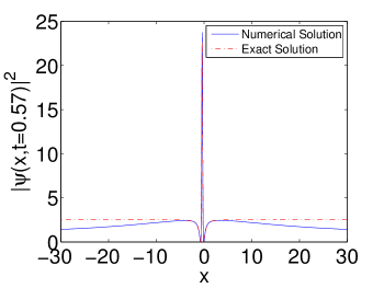
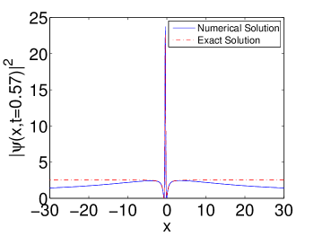
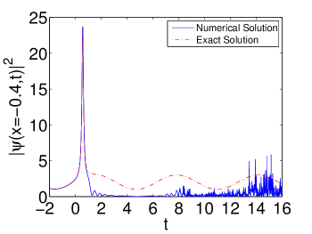
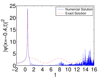
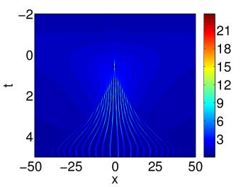
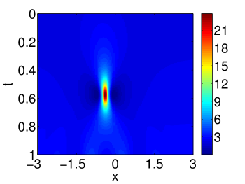
Figure 4. Rogue wave on a periodic background. Left and right panels correspond to numerical results using the DOP853 method and the RK4 one, respectively. The top panels (a-b) show the spatial distribution of the intensity $|\psi|^{2}$ at $t=0.57$, whereas the panels (c-d) show its temporal evolution at $x=-0.4$. The panels (e-h) show contour plots of the density profile of the rogue wave (a wider and a narrower view of the field around the rogue wave is provided).

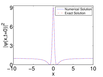
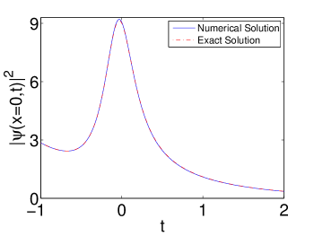
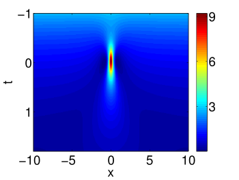
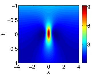
Figure 5. Rogue wave on a monotonically decreasing background. Left and right panels correspond to numerical results using the DOP853 method and the RK4 one, respectively. The top panels (a-b) show the spatial distribution of the intensity $|\psi|^{2}$ at $t=0$, whereas the panels (c-d) show its temporal evolution at $x=0$. The panels (e-h) show contour plots of the density profile of the rogue wave (again, presenting a wider and a narrower space-time view of the density field).

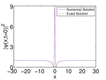
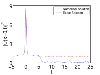
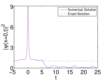
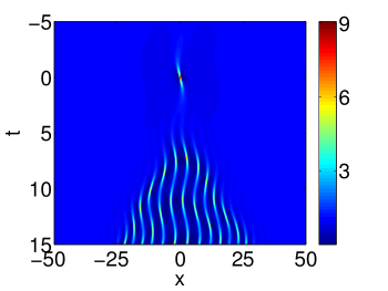
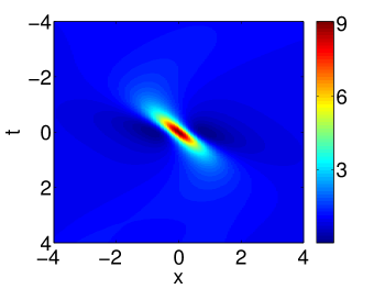
Figure 6. Twisted rogue wave. Left and right panels correspond to numerical results using the DOP853 method and the RK4 one, respectively. The top panels (a-b) show the spatial distribution of the intensity $|\psi|^{2}$ at $t=0$, whereas the panels (c-d) show its temporal evolution at $x=0$. Finally, the panels (e-h) show contour plots of the density profile of the rogue wave.

4. Conclusions

In conclusion, we explored some case examples of rogue wave solutions in NLS systems with variable coefficients. Starting from a general analytical framework, and motivated by the possibility of atomic physics applications in the realm of Bose-Einstein condensates, we focused on NLS models with constant dispersion. Through the choice of arbitrary functions and parameters involved in a transformation of the unknown field, and the use of a “seed solution” of an auxiliary NLS model (in proper coordinates), in the form of a rogue wave, we were led to three different NLS models that we argued as being relevant to the physics of atomic BECs. These models, in particular, may be used to describe BEC settings where the external potential or/and the atomic scattering length (i.e., the nonlinearity coefficient in the NLS model) depend on time. We discussed variants of these possibilities that have already been implemented in actual BEC experiments and which suggest the realizability of our proposed models.

For the above mentioned three different models, exact analytical rogue wave solutions were determined. Our analytical results were also tested against direct numerical simulations. In particular, these solutions were employed as initial conditions for the direct numerical integration of the original NLS equations. We used two different integration schemes, based on the Dormand and Prince (DOP853) method, and the more standard 4th-order Runge-Kutta (RK4) method. The numerical results we obtained by these two methods clearly demonstrated the formation of the rogue waves in close agreement with the analytical results (in both our numerical methods).

This agreement, together with the physical relevance of the considered models, suggest that the predicted rogue waves may have a good chance to be observed within the current experimental capability of BEC setups. That being said, we also observed some very interesting side-products of the Peregrine solitary wave initial data. In particular, the apparent amplification of local truncation errors, especially given the large amplitude of the associated solutions led to significant deviations from the uniform state anticipated (by means of the exact solution) past the formation of the rogue wave in two out of three of our examples. More specifically, the uniform state became subject to a modulational instability initiated exactly at the location of the rogue wave (where the error was apparently amplified maximally). This led to the emergence of an ordered pattern of solitary waves which subsequently expanded spatially as time evolved. This phenomenon was intriguing in its own right and such a nonlinear evolution of small perturbations to the Peregrine profile merits additional investigation both from a numerical but perhaps also from an analytical perspective (at the level of the regular NLS model). This is a natural direction for further studies.

There are many additional directions that would also be relevant and timely. Here, we focused on single Peregrine solitons, while other rogue wave solutions (including periodic ones) and a detailed comparison of their dynamics, would be particularly interesting. Additionally, we explored systems with constant dispersion; nevertheless, systems with varying dispersion that are particularly relevant in the context of optics, would be another theme for future investigations. Finally, a potential generalization of the present settings to higher dimensional configurations would be particularly relevant to consider in numerous physical settings, including fluid and superfluid, as well as nonlinear optical systems. Such studies are currently in progress and will be reported in future publications.

Note added. After the submission of this paper, we were informed of the following relevant works on the modulation of breathers and localized solutions in single and multi-component nonlinear Schrödinger equations: [58]-[60].

Acknowledgments. This work is supported by the NSF of China under Grant No. 11271210 and the K. C. Wong Magna Fund in Ningbo University. The work of D.J.F. was partially supported by the Special Account for Research Grants of the University of Athens. E.G.C. is indebted to both the Institute of Physics, Carl von Ossietzky University (Oldenburg) and the University of Massachusetts (Amherst) for the kind hospitality provided where part of this work was carried out there. He also gratefully acknowledges financial support from the German Research Foundation DFG, the DFG Research Training Group 1620 “Models of Gravity” and FP7 People IRSES-606096: “Topological Solitons, from Field Theory to Cosmos”. P.G.K. also acknowledges support from the National Science Foundation under grants CMMI-1000337, DMS-1312856, from the Binational Science Foundation under grant 2010239, from FP7-People under grant IRSES-606096 and from the US-AFOSR under grant FA9550-12-10332.

References

- [1] C. Kharif and E. Pelinovsky, Eur. J. Mech. B 22, 603 (2003).
- [2] C. Kharif, E. Pelinovsky, and A. Slunyaev, Rogue Waves in the Ocean (Springer, NY, 2009).
- [3] P. K. Shukla, I. Kourakis, B. Eliasson, M. Marklund, and L. Stenflo, Phys. Rev. Lett. 97, 094501 (2006); N. Akhmediev, A. Ankiewicz, and J. M. Soto-Crespo, Phys. Rev. E 80, 026601 (2009); N. Akhmediev, J. M. Soto-Crespo, and A. Ankiewicz, Phys. Rev. A 80, 043818 (2009).
- [4] N. Akhmediev, A. Ankiewicz, and M. Taki, Phys. Lett. A 373, 675 (2009).
- [5] V. Ruban et al., Eur. Phys. J. Special Topics 185, 5 (2010).
- [6] N. Akhmediev, J. M. Dudley, D. R. Solli, and S. K. Turitsyn, J. Opt. 15, 060201 (2013).
- [7] S. W. Xu, J. S. He, L. H Wang, J. Phys. A44, 305203 (2011).
- [8] J. S. He, S. W. Xu, K. Porseizan, Phys. Rev. E 86, 066603 (2012).
- [9] L. J. Li, Z. W. Wu, L. H. Wang, J. S. He, Annals of Physics 334, 198 (2013).
- [10] J. S. He, H. R. Zhang, L. H. Wang, K. Porsezian, A. S. Fokas, Phys. Rev. E 87, 052914 (2013).
- [11] Yu. V. Bludov, V. V. Konotop, and N. Akhmediev, Phys. Rev. A 80, 033610 (2009); Eur. Phys. J. Special Topics 185, 169 (2010); L. Wen, L. Li, Z. D. Li, S. W. Song, X. F. Zhang, and W. M. Liu, Eur. Phys. J. D 64, 473 (2011); Z. Qin and G. Mu Phys. Rev. E 86, 036601 (2012).
- [12] W. M. Moslem, Phys. Plasmas 18, 032301 (2011).
- [13] G. P. Veldes, J. Borhanian, M. McKerr, V. Saxena, D. J. Frantzeskakis, and I. Kourakis, J. Opt. 15, 064003 (2013).
- [14] L. Stenflo and M. Marklund, J. Plasma Phys. 76, 293 (2010).
- [15] Z. Y. Yan, Commun. Theor. Phys. 54, 947 (2010).
- [16] P. T. S. DeVore, D. R. Solli, D. Borlaug, C. Ropers, and B. Jalali, J. Opt. 15, 0640031 (2013).
- [17] M. Onorato, S. Residori, U. Bortolozzo, A. Montinad, and F. T. Arecchi, Physics Reports 528, 47(2013).
- [18] D. R. Solli, C. Ropers, P. Koonath, and B. Jalali, Nature 450, 1054 (2007).
- [19] B. Kibler et al., Nature Phys. 6, 790 (2010).
- [20] B. Kibler et al., Sci. Rep. 2, 463 (2012).
- [21] C. Lecaplain, Ph. Grelu, J. M. Soto-Crespo, and N. Akhmediev, Phys. Rev. Lett. 108, 233901 (2012).
- [22] A. N. Ganshin, V. B. Efimov, G. V. Kolmakov, L. P. Mezhov-Deglin, and P. V. E. McClintock, Phys. Rev. Lett. 101, 065303 (2008).
- [23] A. Chabchoub, N. P. Hoffmann, and N. Akhmediev, Phys. Rev. Lett. 106, 204502 (2011); A. Chabchoub, N. Hoffmann, M. Onorato, and N. Akhmediev, Phys. Rev. X 2, 011015 (2012).
- [24] H. Xia, T. Maimbourg, H. Punzmann, and M. Shats, Phys. Rev. Lett. 109, 114502 (2012).
- [25] M. Shats, H. Punzmann, and H. Xia, Phys. Rev. Lett. 104, 104503 (2010).
- [26] H. Bailung, S. K. Sharma, and Y. Nakamura, Phys. Rev. Lett. 107, 255005 (2011).
- [27] V. E. Zakharov, Zh. Prikl. Mekh. i Tekhn. Fiz. 9, 86 (1968) [J. Appl. Mech. and Tech. Phys. 9, 190 (1968)]; T. B. Benjamin and J. E. Feir, J. Fluid Mech. 27, 417 (1967); G. B. Whitham, J. Fluid Mech. 22, 273 (1965); L. A. Ostrovsky, Sov. Phys. JETP 24, 797 (1967).
- [28] D. H. Peregrine, J. Aust. Math. Soc. B 25, 16 (1983).
- [29] E. A. Kuznetsov, Sov. Phys.-Dokl. 22, 507 (1977).
- [30] Ya. C. Ma, Stud. Appl. Math. 60, 43 (1979).
- [31] N. N. Akhmediev, V. M. Eleonskii, and N. E. Kulagin, Theor. Math. Phys. 72, 809 (1987).
- [32] K. B. Dysthe and K. Trulsen, Phys. Scr. T82, 48 (1999).
- [33] L. P. Pitaevskii and S. Stringari, Bose-Einstein Condensation (Oxford University Press, Oxford, 2003).
- [34] P. G. Kevrekidis, D. J. Frantzeskakis, and R. Carretero-González, Emergent Nonlinear Phenomena in Bose-Einstein Condensates: Theory and Experiment (Springer-Verlag, Heidelberg, 2008); R. Carretero-González, D. J. Frantzeskakis, and P. G. Kevrekidis, Nonlinearity 21, R139 (2008).
- [35] Yu. S. Kivshar and G. P. Agrawal, Optical Solitons: From Fibers to Photonic Crystals (Academic Press, New York, 2003).
- [36] S. Inouye, M. R. Andrews, J. Stenger, H. J. Miesner, D. M. Stamper-Kurn, and W. Ketterle, Nature (London) 392, 151 (1998); J. Stenger, S. Inouye, M. R. Andrews, H.-J. Miesner, D. M. Stamper-Kurn, and W. Ketterle, Phys. Rev. Lett. 82, 2422 (1999); J. L. Roberts, N. R. Claussen, J. P. Burke, Jr., C. H. Greene, E. A. Cornell, and C. E. Wieman, ibid. 81, 5109 (1998); S. L. Cornish, N. R. Claussen, J. L. Roberts, E. A. Cornell, and C. E. Wieman, ibid. 85, 1795 (2000).
- [37] F. K. Fatemi, K. M. Jones, and P. D. Lett, Phys. Rev. Lett. 85, 4462 (2000); M. Theis, G. Thalhammer, K. Winkler, M. Hellwig, G. Ruff, R. Grimm, and J. H. Denschlag, ibid. 93, 123001 (2004).
- [38] S. K. Turitsyn, B. G. Bale, and M. P. Fedoruk, Phys. Rep. 521, 135 (2012).
- [39] Y. V. Kartashov, B. A. Malomed, and L. Torner, Rev. Mod. Phys. 83, 405 (2011).
- [40] V. N. Serkin, A. Hasegawa, and T. L. Belyaeva, Phys. Rev. Lett. 98, 074102 (2007).
- [41] J. Belmonte-Beitia, V. M. Pérez-Garcia,V. Vekslerchik, and P. J. Torres, Phys. Rev. Lett. 98, 064102 (2007).
- [42] J. Belmonte-Beitia, V. M. Pérez-García, V. Vekslerchik, and V. V. Konotop, Phys. Rev. Lett. 100, 164102 (2008).
- [43] S. Rajendran, P. Muruganandam, and M. Lakshmanan, Physica D 239, 366 (2010).
- [44] Z. Z. Yan, Phys. Lett. A 374, 4838 (2010).
- [45] J. S. He and Y. S. Li, Stud. Appl. Math. 126, 1 (2011).
- [46] S. W. Xu, J. S. He, L. H. Wang, Europhys.Lett. 97, 30007(2012).
- [47] J. S. He, Y. S. Tao, K. Porsezian, A. S. Fokas, J. Nonlinear Mathematical Physics 20, 407(2013).
- [48] Z. Yan, Phys. Lett. A 374, 672 (2010).
- [49] K. E. Strecker, G. B. Partridge, A. G. Truscott, and R. G. Hulet, Nature (London) 417, 150 (2002); New J. Phys. 5, 73 (2003).
- [50] L. Khaykovich, F. Schreck, G. Ferrari, T. Bourdel, J. Cubizolles, L. D. Carr, Y. Castin, and C. Salomon, Science 296, 1290 (2002).
- [51] S. L. Cornish, S. T. Thompson, and C. E. Wieman, Phys. Rev. Lett. 96, 170401 (2006).
- [52] J. W. Fleischer, M. Segev, N. K. Efremidis, and D. N. Christodoulides, Nature (London) 422, 147 (2003); D. Neshev, T. J. Alexander, E. A. Ostrovskaya, Yu. S. Kivshar, H. Martin, I. Makasyuk, and Z. Chen, Phys. Rev. Lett. 92, 123903 (2004).
- [53] M. Centurion, M. A. Porter, P. G. Kevrekidis, and D. Psaltis, Phys. Rev. Lett. 97, 033903 (2006); M. Centurion, M. A. Porter, Y. Pu, P. G. Kevrekidis, D. J. Frantzeskakis, and D. Psaltis, ibid. 97, 234101 (2006).
- [54] B. P. Anderson and M. A. Kasevich, Science 282, 1686 (1998).
- [55] H. Lignier, C. Sias, D. Ciampini, Y. Singh, A. Zenesini, O. Morsch, and E. Arimondo, Phys. Rev. Lett. 99, 220403 (2007).
- [56] Q.-Y. Li, Z.-D. Li, S.-X. Wang, W.-W. Song, and G. Fu, Opt. Commun. 282, 1676 (2009).
- [57] E. Hairer, S. P. Nørsett and G. Wanner, Solving ordinary differential equations I (Springer-Verlag, Berlin, 1993).
- [58] A. T. Avelar, D. Bazeia, and W. B. Cardoso, Phys. Rev. E 82, 057601 (2010).
- [59] W. B. Cardoso, A. T. Avelar, and D. Bazeia, Phys. Lett. A 374, 2640 (2010).
- [60] W. B. Cardoso, A. T. Avelar, and D. Bazeia, Phys. Rev. E 86, 027601 (2012).