MyGIsFOS: an automated code for parameter determination and detailed abundance analysis in cool stars

Abstract

Context. The current and planned high-resolution, high-multiplexity stellar spectroscopic surveys, as well as the swelling amount of under-utilized data present in public archives have led to an increasing number of efforts to automate the crucial but slow process to retrieve stellar parameters and chemical abundances from spectra.

Aims. We present MyGIsFOS, a code designed to derive atmospheric parameters and detailed stellar abundances from medium - high resolution spectra of cool (FGK) stars. We describe the general structure and workings of the code, present analyses of a number of well studied stars representative of the parameter space MyGIsFOS is designed to cover, and examples of the exploitation of MyGIsFOS very fast analysis to assess uncertainties through Montecarlo tests.

Methods. MyGIsFOS aims to reproduce a “traditional” manual analysis by fitting spectral features for different elements against a precomputed grid of synthetic spectra. Fe i  and Fe ii lines can be employed to determine temperature, gravity, microturbulence, and metallicity by iteratively minimizing the dependence of Fe i abundance from line lower energy and equivalent width, and imposing Fe i-Fe ii ionization equilibrium. Once parameters are retrieved, detailed chemical abundances are measured from lines of other elements.

Results. MyGIsFOS replicates closely the results obtained in similar analyses on a set of well known stars. It is also quite fast, performing a full parameter determination and detailed abundance analysis in about two minutes per star on a mainstream desktop computer. Currently, its preferred field of application are high-resolution and/or large spectral coverage data (e.g UVES, X-Shooter, HARPS, Sophie).

1 Introduction

The availability of several high-efficiency, high-multiplexity spectrographs has brought about the need to perform accurate abundance analysis on large sets of stellar spectra of low to high resolution. The problem has been tackled in many different ways, one may roughly divide the methods into “global”, that make use of the whole spectrum (e.g. Katz et al., 1998; Allende Prieto et al., 2000; Bailer-Jones, 2000; Recio-Blanco et al., 2006) and “local”, that make use only of selected sections of the spectrum (e.g. Erspamer & North, 2002; Bonifacio & Caffau, 2003; Barklem et al., 2005; Boeche et al., 2011; Posbic et al., 2012; Mucciarelli et al., 2013; Magrini et al., 2013). A few “intermediate” cases exist, most notably SME (Valenti & Piskunov, 1996; Barklem et al., 2005), underlining perhaps the difficulty to come up with a clear-cut classification scheme. Complex pipelines, like that of the Sloan Digital Sky Survey (Allende Prieto et al., 2008) use multiple methods whose results are then suitably combined. Among the “local” codes one may distinguish between those that rely on equivalent widths (EWs) measured by automatic codes such as fitline (François et al., 2003), DAOSPEC (Stetson & Pancino, 2008) or ARES (Sousa et al., 2007) to determine stellar parameters and abundances (Mucciarelli et al., 2013; Magrini et al., 2013), and those that rely on line-fitting (Erspamer & North, 2002; Bonifacio & Caffau, 2003; Barklem et al., 2005; Boeche et al., 2011; Posbic et al., 2012; Van der Swaelmen et al., 2013). Allende Prieto (2004) argued that EW based analysis should be abandoned, see also Bonifacio (2005) on EWs and line-fitting.

We present in this paper the code MyGIsFOS that uses a “local” approach to treat large numbers of medium to high-resolution spectra. Among the “local” codes MyGIsFOS  Abbo (Bonifacio & Caffau, 2003), and the RAVE pipeline of Boeche et al. (2011) are the only ones, to our knowledge, that do not perform “on-the-fly” line transfer computations, but rely only on a pre-computed grid. In the Boeche et al. (2011) pipeline, a library of synthetic curves of growth are compared to the measured EW of the chosen observed lines. In this sense, this code is closer to EW-based ones as far as line selection criteria, advantages, and limitations are concerned, but faster than most EW-based codes since no on-the-fly line transfer is performed.

MyGIsFOS and Abbo, on the other hand, directly fit the synthetic profile of each chosen feature against the observed one. As such, they allow to circumvent some of the limitations of EW-based codes (see, e.g., Sect. 5.1), while, at the same time, maintaining the speed advantage of codes not performing on-the-fly calculations.

At the same time, the RAVE pipeline, MyGIsFOS and Abbo suffer of limitations inherent to the use of pre-computed grids. Namely, these grid can become exceedingly large, or must be limited in parameter space range. Moreover, precomputed grids are by their nature “rigid”: their computation is resource intensive, and recomputation for the purpose of changing, for instance, one of two line oscillator strength might not be a desirable option.

For all these reasons, such codes are optimized to analyze a large number of stars that span a limited range in metallicity, effective temperature and surface gravity.

MyGIsFOS specifically targets the treatment of large amounts of data, through a local approach, based on spectrum synthesis, line profile fitting and a pre-computed synthetic spectrum grid. Although other procedures exist that incorpoarate these feature none exists that uses at the same time all of these features. In this case we believe MyGIsFOS is unique and innovative.

2 The purpose of MyGIsFOS

MyGIsFOS  is built on the foundation of our previous automatic abundance analysis code Abbo (Bonifacio & Caffau, 2003). Although it has been completely rewritten, has a different input-output system and it is considerably more powerful and faster, the scope of the code is unchanged with respect to Abbo. Broadly speaking, the observed spectrum is compared against a suitable grid of synthetic stellar spectra which have been computed at varying $T_{\mathrm{eff}}$, $\log g$, V_turb, [Fe/H], [$\alpha$/Fe]. Selected Fe i, Fe ii, and $\alpha$-elements features are used to iteratively estimate the best values for each parameter, after which features for other elements are fitted to derive the corresponding abundances.

Table 1: The MyGIsFOS grids computed with SYNTHE and ATLAS 12 models employed for the present paper.

Grid	$T_{\mathrm{eff}}$	$\log g$	Vturb	[Fe/H]	[$\alpha$/Fe]	Number of
name	range	range	range	range	range	models
	[K]	[c.g.s.]	[ km s-1]
Metal Poor Cool Dwarfs	5000 to 6000	3 to 5	0 to 3	-4 to -0.5	-0.4 to 0.8	3840
(MPCD)	step 200 K	step 0.5	step 1	step 0.5	step 0.4
Metal Rich Cool Dwarfs	5000 to 6000	3 to 5	0 to 3	-1 to 0.75	-0.4 to 0.8	3840
(MRCD)	step 200 K	step 0.5	step 1	step 0.25	step 0.4
Metal Poor Giants	4200 to 5600	1 to 3	1 to 3	-4 to -0.5	-0.4 to 0.4	2880
(MPG)	step 200 K	step 0.5	step 1	step 0.5	step 0.4
Metal Rich Giants	4200 to 5600	1 to 3	1 to 3	-1 to 0.5	-0.4 to 0.4	2520
(MRG)	step 200 K	step 0.5	step 1	step 0.25	step 0.4

MyGIsFOS  is conceived to strictly replicate a “classical” or “manual” procedure to derive stellar atmospheric parameters and detailed chemical abundances from high resolution stellar spectra of cool stars. As such, its most typical usage case can be resumed as follows:

• For each star to be analyzed, the user provides input observed spectrum and a set of first guess parameters.

• The user provides the code a feature list, i.e. a list of spectral intervals for the grid to be fitted against the observed spectrum. In the most general case the feature list will include continuum intervals for pseudo-normalization and signal-to-noise ratio (S/N) estimation, intervals corresponding to Fe i  Fe ii  and $\alpha$-element lines for atmospheric parameter and metallicity ([Fe/H]) determination, and intervals corresponding to lines of other elements for the determination of detailed abundances.

• $T_{\mathrm{eff}}$  is determined from a set of isolated Fe i lines imposing the linear fit of the transition lower energy vs. line abundance to have null slope (for brevity, we will henceforth refer to this quantity as Lower Energy Abundance Slope, or LEAS).

• V_turb is determined by imposing null slope for the Equivalent Width (EW) vs. abundance relation of isolated Fe i lines.

• $\log g$ is determined from Fe i- Fe ii ionization equilibrium.

• Fe abundance is determined from Fe i lines only.

• [$\alpha$/Fe] is determined by measuring lines of various $\alpha$ elements, and using their average [X/Fe] as an estimate of [$\alpha$/Fe].

• V_turb, $\log g$, and [$\alpha$/Fe] are estimated iteratively, in a nested fashion, [$\alpha$/Fe] being the outermost “shell”, V_turb the innermost. For a given set of current guesses of $T_{\mathrm{eff}}$, $\log g$, and $\alpha$ enhancement, V_turb is determined, then the code passes to update the gravity estimate: if the current one is not appropriate, a new one is guessed, V_turb is redetermined by assuming the new gravity and the existing estimates for the other parameters, then gravity is tested again. When a satisfactory estimate is reached for both V_turb and $\log g$, [$\alpha$/Fe] is tested, and if changed, a recalculation of V_turb and $\log g$ is triggered.

• $T_{\mathrm{eff}}$ is evaluated in a slightly different fashion: initially, the aforementioned analysis is repeated to full convergence assuming a set of different temperatures, and in each case, the LEAS is derived. This intial “mapping” is used to fit the $T_{\mathrm{eff}}$-LEAS relationship and look for a zero-slope temperature, which is then used to repeat the V_turb, $\log g$, [$\alpha$/Fe] determination. The LEAS is evaluated again and the estimated slope added to the $T_{\mathrm{eff}}$-LEAS relationship fitting sample. A zero is searched again and so on, until convergence is reached.

• Any of the aforementioned parameters can be either derived as described from the spectrum, or kept fixed at a user-defined value. MyGIsFOS will of course refrain to alter parameters for which the corresponding estimator is absent, e.g. gravity will not be estimated if no Fe ii features are successfully measured. Thus, the user does not need to provide features for any parameter he/she is not planning to alter, the only exception being Fe i features, which should always be present ([Fe/H] cannot be kept fixed).

• The whole analysis is executed in a fully automated way for all the stars in the input list and the output is stored in a separate directory for each star. The input star list should contain data of similar quality and spectral range (e.g. UVES red-arm spectra with S/N$\sim$ 50-100, for a description of UVES see Dekker et al., 2000), and of objects of comparable characteristics (say, metal-rich FGK dwarfs), because feature list, general running parameters (e.g. fit rejection tolerances) and synthetic spectra grid are common to the input star list and should thus be appropriate for all the objects. The constraints on S/N ratio, spectral type and metallicity, are not very tight. Experiments with real UVES spectra have shown that if the feature list has been optimized for S/N in the range 50-100 it can works well for S/N in the ratio 15-300. At the low S/N ratio most of the selected features are not detected because too weak and one has to switch to a selection of strong, saturated lines. At the high S/N ratio end it is useful to add many weak lines that are not detectable at lower S/N. For the atmospheric parameters the main constraint is metallicity, since features that are heavily blended become much cleaner and are usable at lower metallicity, at the same time features that are saturated in the high metallicity regime reach the linear part of the curve of growth at lower metallicity. The switch-over between metal-rich and meal-weak regime happens somewhere between [M/H] –0.5 and –1.0. MyGIsFOS is designed to analyse data sets for which we have some previous knowledge (colours, metallicity estimates, membership to a cluster or dwarf galaxy) our experience is that in these cases the stars that need to be re-run a second time because initially misclassified is less than 5%.

It is then clear that the ideal application of MyGIsFOS is the determination of detailed chemical abundances from high to intermediate resolution spectra of cool stars, with basically the same limitations and strengths as a traditional “manual” analysis: the results will be of higher quality if the spectral coverage is large, if S/N ratio is good, if clean, unblended features are chosen. Few, noisy or anyway unreliable Fe ii lines will make gravity estimation difficult, the quality of the adopted atomic data will impact the precision of any abundance derived, and so on. On the other hand, MyGIsFOS results are immediately comparable with the ones derived from a traditional abundance analysis. Uncertainties, limitations, and dependence from the assumption made in atmosphere modeling and spectrosynthesis are well known, and researchers in the field are since long used to deal with them. This makes MyGIsFOS output easy to test, interpret, and compare with the results from previous works, advantages MyGIsFOS  shares with EW-based automation schemes such as FAMA or GALA.

MyGIsFOS produces an extensive output (in ASCII format) for each star to allow for critical examination of the analysis outcome. Included are detailed information on each feature fitted (best fitting line profile, abundance, EW, rejection flags and quality-of-fit estimators), pseudo-normalized input spectra and best-fitting synthetic spectra, as well as averaged abundances and parameters in tabular form, and a full listing of all the input parameters, employed grid characteristics, and code version. Also, all output files from the same run share a timestamp to ease tracking.

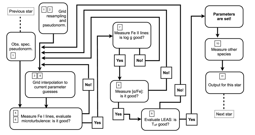
Figure 1: A schematic flowchart of MyGIsFOS. Numbers in rectangles refer to the MyGIsFOS phases enumeration given in Sect. 4.

Thanks to the use of a fully precomputed synthetic grid, MyGIsFOS is remarkably fast: a typical run on a standard desktop computer, with full parameter determination and $\sim$20 element abundances, for 200nm high-resolution optical spectra takes about 120s per star (see Sect. 8 for more details).

3 The synthetic spectra grid

MyGIsFOS  works by comparing selected spectral features with a grid of synthetic stellar spectra with varying $T_{\mathrm{eff}}$, $\log g$, V_turb, [Fe/H], and [$\alpha$/Fe]. The grid is provided as an unformatted binary file that reduces physical size and read-in time. The grid contains a header containing a comment, the grid “metrics” (starting point, step and number of steps in each parameter), the assumed solar abundances, the elements affected by $\alpha$ enhancement and the assumed grid instrumental broadening. The grid should be passed as already broadened as needed by the spectrograph resolution. The grid is in general divided into several spectral ranges or “frames”. This is foreseen to handle situations in which only limited, non contiguous spectral ranges are needed, such as when treating data from different settings of single-order, high multiplexity spectrographs such as FLAMES@VLT (Pasquini et al., 2002). If this is not needed, the grid might contain a single frame covering the needed spectral range. The frame subdivision is also indicated in the grid header, that then contains all the information needed by MyGIsFOS  to read in the grid data without user intervention.

The grid should be passed to MyGIsFOS  at high sampling ($\Delta\lambda/\lambda>$100000) to prevent the arising of artifacts when it is resampled over the actual observed data points.

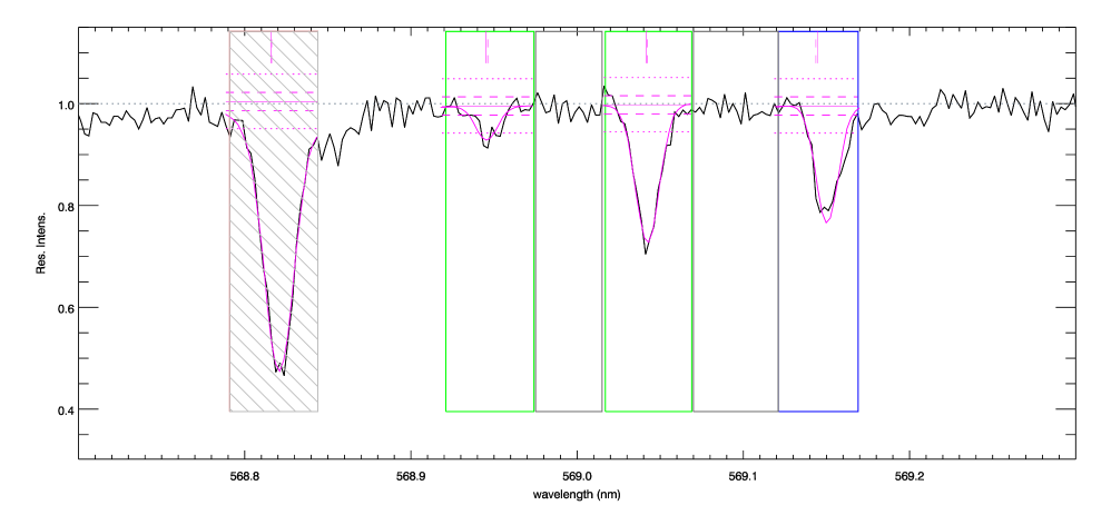
Figure 2: A small section of the S/N=50 solar spectrum presented in 6.1 with overplotted MyGIsFOS features and fitting result, as produced by the ancillary plotting package SQUID. From left to right: a rejected Na i line (rejected due to EW exceeding the applied maximum EW constraint, gray shaded box); a Ti i feature (green box); a continuum interval (gray box); a Si i feature (green box again); another continuum (gray); a Fe i features (blue box). The observed spectrum (black line) appears as renormalized by MyGIsFOS. The gray dashed horizontal line represents the continuum level, each feature is superimposed with the best fit synthetic (magenta), the best fit continuum (magenta continuous horizontal line), 1-$\sigma$ and 3-$\sigma$ values of the noise (horizontal dashed and dotted magenta lines), and markers of best fit doppler shift for the feature (magenta vertical continuous and dashed lines).

For all the tests presented in this paper we computed a set of model atmospheres and synthetic spectra appropriate for the analysis of FGK stars, both dwarfs and giants, over a wide range of metallicities. The atmospheric models have been computed with the Linux version of ATLAS 12, while synthetic spectra covering the UVES RED 580 setting (approx 480 to 680 nm) have been computed by means of SYNTHE (Kurucz, 2005; Castelli, 2005; Sbordone et al., 2004; Sbordone, 2005). Parameter space coverage of the used grids to date are listed in Table 1. Models and syntheses have been computed in a self-consistent way, i. e. changes in V_turb and [$\alpha$/Fe] have been included already in the opacity computation during model calculation. Assumed solar abundances are derived from Caffau et al. (2011B) for the elements there analyzed, and from Lodders et al. (2009) for the remaining species. The used grids are part of a larger set being currently prepared for publication (Sbordone et al.,, 2013). Synthetic grids are computed with sampling $\Delta\lambda/\lambda$=300000 in the 460nm - 690nm range, and take in their binary packaged version between 1.5 and 2.2 GB of space.

4 The MyGIsFOS workflow in detail

As above stated, MyGIsFOS replicates classical “manual” abundance analysis workflow. User defined parameters are read from an ASCII parameter file. A flowchart of the process for a single star is shown in Fig.1, while an example of the result is given in Fig. 2. The workflow can be summarized as follows:

1. The observed spectrum (or spectra) is pseudonormalized by evaluating the pseudo-median of each continuum interval. A continuum value is then calculated for each observed pixel by computing a spline through all the continuum intervals. Also, from every continuum interval the local S/N ratio is estimated. The whole synthetic grid is pseudo-normalized in the same way. The pseudonormalization is kept fixed throughout the analysis of the star.

2. The synthetic grid is then resampled at the wavelengths of each observed pixel.

3. The first value for effective temperature estimation is chosen. If $T_{\mathrm{eff}}$ is kept fixed for the star, said value is the initial guess provided as input, and is never changed afterwards. Otherwise, MyGIsFOS begins scanning the $T_{\mathrm{eff}}$-LEAS relationship. This can be performed in two modes: either each $T_{\mathrm{eff}}$ in the grid is tried (full scan mode), or only a few hundreds K around the initial estimate are tried (local scan mode). To do so, for each temperature probed $\log g$, V_turb, [Fe/H], and [$\alpha$/Fe] are determined (steps between 4 and 8 below), then the LEAS is determined (step 9 below). The operation is repeated for each $T_{\mathrm{eff}}$ to be scanned. After the scan is completed, MyGIsFOS begins to refine its temperature estimate by fitting the $T_{\mathrm{eff}}$-LEAS relationship with a 2nd order polynomial and estimating the zero-LEAS $T_{\mathrm{eff}}$ value. Each new attempt is added to the sample, the fit repeated and the new zero determined. Search stops when step-to-step $T_{\mathrm{eff}}$ change is less than a threshold parameter value (typically, 50K).

4. At the beginning of the actual line measurement stage, the synthetic grid is interpolated at the current guess values for $T_{\mathrm{eff}}$, $\log g$, V_turb, and [$\alpha$/Fe]. As a consequence, it is now reduced to a set of synthetic spectra with equal atmosphere parameters but varying metallicity.

5. A set of Fe i lines is measured: for each feature, the set of synthetic spectra at varying metallicity is compared against the observed spectrum and the best fit determined by $\chi^{2}$ minimization allowing three free parameters: metallicity, a small radial velocity shift, and a small deviation from the established continuum value, never to surpass a given fraction of the local S/N ratio. Local S/N is evaluated by fitting a 3rd order polynomial to all the S/N estimates in the relevant observed frame. Also, EW is determined for both the observed and best fitting synthetic feature by direct integration under the pseudo-continuum. EWs will be used in some of the line rejection criteria, and in the search for the best microturbulence, see below. Measurement for each feature is kept if a number of criteria are met: i) the fit probability should exceed a given threshold, ii) the equivalent width of the observed and fitted synthetic line should not differ by more than a given threshold, iii) both the observed and the synthetic EWs should exceed a given value, iv) both EWs should exceed a certain number of times the EW of a noise-dominated line and v) EW should not exceed a user-defined maximum value EW_max, to allow avoiding using heavily saturated lines. If any of the above tests fails, the feature is marked for rejection. The same rejection criteria will be applied also to features for every other elements later on in the analysis.

6. Once all the assigned Fe i features have been measured, the average of their abundance is computed, and $\sigma$-clipping performed (every feature deviating more than $n\sigma$ from the average is rejected, $n$ being set as one of MyGIsFOS input parameters). After the $\sigma$-clipping phase, a linear fit is performed in the EW-A(Fe) plane to determine microturbulence. Step 5 and 6 are performed at least four times: the first time measuring Fe i lines at the grid’s lowest microturbulence value, the second time at the highest, the third at the zero of the linear fit of the first two, the fourth at the zero of the 2nd order fit of the first three. In a fashion similar to what described for $T_{\mathrm{eff}}$ in step 3 every time a new V_turb is evaluated, it is added to the sample and a 2nd order polynomial is fitted again to the whole set. We do not seek the minimum slope of the linear EW-A(Fe) relationship, but when it is smaller than the threshold set in the parameter file, microturbulence is considered determined, as well as Fe i abundance.

7. Step 4 is repeated again at the established microturbulence, and Fe ii lines are measured. Their average, $\sigma$-clipped abundance is compared with the average Fe i abundance. If their discrepancy exceed the threshold set in the parameter file, a new gravity is estimated from the size of said discrepancy and steps 4, 5, and 6 are repeated until a new value of microturbulence and Fe i abundance are found with the new gravity. Fe i and Fe ii abundances are compared again, and the process is repeated until convergence is reached.

8. With the current estimates of microturbulence and gravity, lines are measured for all the $\alpha$ element ions chosen to estimate $\alpha$ enhancement (we speak of ions because, for instance, one might choose to estimate $\alpha$ enhancement from Mg i and Ti ii). Average, $\sigma$-clipped abundances for each ion are determined, and their respective [X/Fe] are averaged to estimate [$\alpha$/Fe]. Steps 4 to 7 are repeated and all the parameters established again at the newly estimated $\alpha$ enhancement. The $\alpha$ enhancement itself is computed again and compared with the previous value. The process is iterated until the difference is below the threshold set in the parameter file.

9. Now the LEAS is determined with the current parameters, and MyGIsFOS goes back to step 3 if $T_{\mathrm{eff}}$ is being derived.

10. Now the full set of atmospheric parameters is established, and abundances are measured for all the features of all the other ions given in the linelists but not yet measured, again by $\chi^{2}$ fitting of the line profiles. When more than one featrure is available for a ion they are averaged, $\sigma$-clipped, and averaged again to determine the final value of the abundance of that ion.

11. Output files are created, and MyGIsFOS moves on to analyze the next star.

Summarizing the procedure is composed of several “blocks” that have to be iterated: steps 3-9 can be viewed as the “temperature block”, steps 5-6 are the “metallicity block”, step 6 is the “microturbulence block”, steps 5-7 are the “gravity block” and steps 5-8 are the “alpha-enhancement block”.

Table 2: Test of the ability of MyGIsFOS to correctly retrieve Ca i abundances deviating from the assumed solar-scaled composition.

Input	offset from	Retrieved	$\sigma$
[Ca/Fe]	model value	[Ca/Fe]
–0.5	–0.9	–0.52	0.05
–0.2	–0.6	–0.23	0.05
0.1	–0.3	0.07	0.04
0.4	0.0	0.39	0.04
0.7	0.3	0.70	0.04
1.0	0.6	1.00	0.04
1.3	0.9	1.29	0.05

4.1 Comments on the MyGIsFOS workflow

The method for fixing the microturbulence is essentially the same as in Mucciarelli et al. (2013). The advantage of automatising a “classical” approach, rather than a global $\chi^{2}$ minimisation, such as done in SME (Valenti & Piskunov, 1996) or TGMET (Katz et al., 1998) is that in the classical approach the different diagnostics (for $T_{\mathrm{eff}}$, $\log g$, microturbulence, abundances) are kept separate, in a global $\chi^{2}$ minimisation they are all considered together, and it is diffcult to break degeneracies. In the case information other than the spectra can be used (e.g. distances), some parameters can be easily and neatly fixed in the classical approach, less so in a global approach. MyGIsFOS has the same advantage over other, non $\chi^{2}$ based, global methods (Allende Prieto et al., 2000; Bailer-Jones, 2000; Recio-Blanco et al., 2006) that are indeed very fast, but cannot easily break degeneracies. Van der Swaelmen et al. (2013) do not use $\chi^{2}$ fitting but minimise another quantity, that is similar to $\chi^{2}$ (see their section 4.1), as a consequence they cannot use the theorems of $\chi^{2}$ to estimate the goodness of fit.

5 Specifics and limitations

5.1 Features vs. lines

MyGIsFOS operates on spectral features rather than spectral lines. Technically, the fitter at its core compares an observed spectral range against a set of synthetic profiles of the same range varying in [Fe/H] (more on this in Sect. 5.2), and determines the [Fe/H] value for which the fit is best. As such, MyGIsFOS can fit blended features without problems, but, at the same time, it is unable to perform deblending.

The first characteristic comes in handy e. g. when the user wants to derive an overall metallicity from low resolution spectra, because complex blends can be used as metallicity indicators. Another example is the case in which important lines (e. g. the only line available for an element one wants to measure) are blended with some other feature. And of course, MyGIsFOS has no problem fitting lines affected by Hyper Fine Splitting (HFS), provided HFS has been included when the synthetic grid has been computed. Naturally, the quality of the fit of a blend will depend on how well the atomic data of all the relevant features are known. It is also important to keep in mind that element-to-element ratios are kept fixed to the ones set in the grid (with the relevant exception of [$\alpha$/Fe]), which could skew the result of fitting a blend if the two elements involved are not present in the star’s atmosphere with a ratio similar to the one assumed in the grid.

The inability to perform deblending is relevant in any situation where the EW of a line is important, the most obvious case being V_turb determination, which uses the EW of Fe i lines. MyGIsFOS determines two EWs for each feature it measures: one for the observed spectrum feature, and one for the best-fitting synthetic. Both are computed by direct integration under the local continuum value, and their difference is among the criteria used to reject a fit (see Sect. 4, point 5). For Fe i features, EW is then used to estimate V_turb. However, if a feature is a blend, its total EW will be too large in comparison to the associated abundance, skewing the V_turb fit. For this reason, the user is allowed to decide which Fe i features to use for V_turb estimation, and must restrain to use only features corresponding to bona fide isolated Fe i lines.

Table 3: Determined abundances for Sun, Arcturus, and HD 126681.

	Sun: $T_{\mathrm{eff}}$=5794, $\log g$=4.55,			Arcturus: $T_{\mathrm{eff}}$=4293 $\log g$=1.84			HD 126681 $T_{\mathrm{eff}}$=5530, $\log g$=4.41,
	Vturb=1.07, [$\alpha$/Fe]=0.05			Vturb=1.44, [$\alpha$/Fe]=0.19			Vturb=0.50, [$\alpha$/Fe]=0.38
	Number of	[Fe/H] or	$\sigma$	Number of	[Fe/H] or	$\sigma$	Number of	[Fe/H] or	$\sigma$
	features	[X/Fe](a)		features	[X/Fe](a)		features	[X/Fe](a)
Fe i	84	-0.06	0.059	59	-0.44	0.073	116	-1.24	0.087
Fe ii	14	-0.05	0.094	10	-0.44	0.083	14	-1.23	0.069
Na i	3	0.06	0.069	1	0.01	–	4	-0.13	0.140
Mg i	–	–	–	–	–	–	1	0.60	–
Al i	3	-0.04	0.073	2	0.13	0.177	1	0.18	–
Si i	2	0.20	0.12	8	0.33	0.123	6	0.35	0.096
Si ii	–	–	–	2	0.34	0.239	1	0.57	–
Ca i	8	0.02	0.074	1	0.05	–	10	0.40	0.093
Ti i	23	0.04	0.086	4	0.20	0.100	22	0.31	0.120
Ti ii	9	0.11	0.222	2	0.23	0.157	10	0.32	0.250
Ni i	18	0.02	0.153	6	0.02	0.126	15	-0.03	0.172

In a similar fashion, the user will indicate which Fe i lines to employ for $T_{\mathrm{eff}}$ estimation. In a blend of two Fe i features, for instance, one might not meaningfully associate one single lower energy value. Also, it is customary to refrain from using low excitation lines in $T_{\mathrm{eff}}$ estimation, given their general tendency to be prone to stronger departures from local thermodynamical equilibrium (LTE). In diagnostic plots for the test stars (Sect. 6, Figs. 5 trough 10) lines used or rejected in the $T_{\mathrm{eff}}$ and V_turb fitting are clearly indicated.

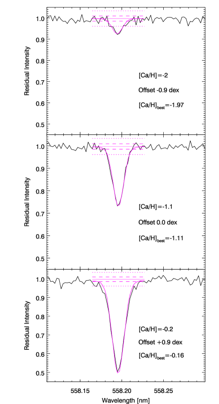
Figure 3: Ca i 559.19 nm line in the case of the two most extreme offsets described in Sect. 5.2 and in the no-offset case, with their respective best fitting synthetic value (magenta profiles). The magenta horizontal lines represent local continuum, one-$\sigma$, and three-$\sigma$ of the local simulated noise. [Ca/H] is the input value, [Ca/H]_best the best fit value for the line.

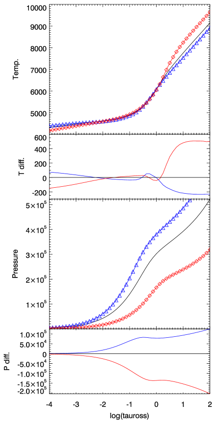
Figure 4: Comparison of Atlas 12 atmosphere models with $T_{\mathrm{eff}}$=5600 $\log g$=4.5, V_turb=1.0, [$\alpha$/Fe]=+0.4 and [Fe/H]=$-2.5$ (blue line and triangles), [Fe/H]=$-1.5$ (black line), and [Fe/H]=$-0.5$ (red line and diamonds).Top to bottom: Temperature for the three models, Temperature difference (red line, [Fe/H]=$-0.5$ – [Fe/H]=$-1.5$; blue line, [Fe/H]=$-2.5$ – [Fe/H]=$-1.5$), pressure in g cm^-2, pressure difference, all plotted vs. $\tau_{\mathrm{ross}}$.

5.2 Metallicity vs. abundance in line fitting

MyGIsFOS computes abundances for lines of all elements by means of a grid which has only two degrees of freedom in chemical composition: metallicity and $\alpha$ enhancement. In fact, every line is fitted against metallicity only. Since all abundances scale the same way with metallicity in the grid (with the exception of $\alpha$ enhancement) MyGIsFOS interprets the result of the fit as due only to the change in the abundance of the specific ion producing the feature. By doing so, MyGIsFOS assumes that varying [Fe/H] but keeping [X/Fe] constant produces the same effect on the line profile than varying [X/Fe] while keeping [Fe/H] constant, or, in other words, it neglects the effect on the atmospheric structure of varying the overall star metallicity. This allows MyGIsFOS to drastically reduce the number of degrees of freedom in the grid, while still being able to measure abundances for an arbitrary number of ions. Otherwise, the grid should grow one dimension for every element which can be measured. This would either impose to use grids with a quite limited parameter span (which is undesirable when searching for optimal atmospheric parameters), or to use much larger grids, which are expensive to calculate, read in, and process inside MyGIsFOS. Moreover, with memory requirements being the bottleneck in running the code (see Sect. 8), such very large grids would rapidly become unwieldy.

The MyGIsFOS approximation thus remains valid as long as the measured abundance does not depart much from the grid solar-scaled composition, since this implies that the synthetic line profile is computed on the basis of an atmosphere which is not much different from the one providing the overall best parameter fit. To provide an indicative estimate of how “safe” the approach is, we have computed a series of synthetic spectra around parameters typical of a metal poor dwarf ($T_{\mathrm{eff}}$=5600 K, $\log g$=4.5, V_turb=1.0, [Fe/H]=–1.5, [$\alpha$/Fe]=+0.4) and changing the Ca abundance to offsets of $\pm$ 0.3, 0.6, and 0.9 dex (since in the starting model [Ca/Fe]=+0.4, this corresponds to [Ca/Fe]=-0.5 to +1.3, and [Ca/H]=–2.0 to –0.2). The spectra were noise-injected to S/N=80 and fed to MyGIsFOS. First, the spectrum without Ca offset was analyzed with full parameter determination to determine how close MyGIsFOS would go to the input values, returning $T_{\mathrm{eff}}$=5580 K, $\log g$=4.41, V_turb=0.88, [Fe/H]=$-1.49$, [$\alpha$/Fe]=0.39, values well in line with the typical offset to be expected as a result of noise injection (see 7.2). Then parameters were locked to the input values, and MyGIsFOS was used to derive abundances only, to see whether the Ca offsets would be retrieved properly despite the Abundance-vs.-Metallicity approximation. The result of the test are presented in Table 2 and, for a specific Ca i line, in Fig. 3. For the specific case, the approximation applied appears to produce no detectable effect on the ability of MyGIsFOS to properly measure abundances deviating for the assumed solar-scaled composition.

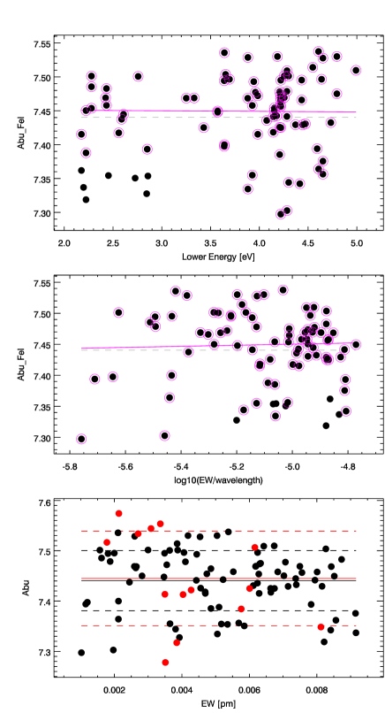
Figure 5: Diagnostic plots for the determination of atmospheric parameters for the Sun. Upper panel: Fe i lines abundances vs. their lower energy and linear fit for the determination of $T_{\mathrm{eff}}$. Gray dashed line, average Fe i abundance. The magenta line is the linear fit, magenta-circled points are the ones considered in the fit. LEAS is $-8.0\leavevmode\nobreak\ 10^{-4}$ per eV. Center panel, Fe i lines abundances vs. reduced EW (i. e. $\log_{10}\left(EW/\lambda\right)$ ) for the determination of V_turb. Gray dashed line, average Fe i abundance. Magenta symbols and line as in the top panel. Linear fit slope is $8.7\leavevmode\nobreak\ 10^{-3}$. Bottom panel, Fe i (black) and Fe ii (red) lines abundances for the check of gravity through ionization equilibrium. Continuous line represent averages, dashed lines $1\sigma$ intervals. A(Fe i)$=7.44\leavevmode\nobreak\ \pm 0.06$, A(Fe ii)$=7.45\leavevmode\nobreak\ \pm 0.09$.

We want to stress that the presented case is not necessarily representative for any possible line being analyzed. For instance, if the line being fitted is significantly blended, in the synthetic grid being fitted against the observed both the “main” feature and the blending ones will vary, which would lead to skewed resulting abundances for any element deviating significantly form solar-scaled abundance. Also, the degree of sensitivity to the MyGIsFOS approximation depends on the physics of line formation for the specific feature. In Fig. 4 we show the comparison of three atmospheric models from our grid very close to the ones of interest in this comparison. The “central” model is the one used to compute all the simulated observed spectra considered in this section ($T_{\mathrm{eff}}$=5600 K, $\log g$=4.5, V_turb=1.0, [Fe/H]=$-1.5$, [$\alpha$/Fe]=+0.4). The other two differ in metallicity only, being offset by 1 dex upards and downwards, thus being representative of the $\pm$ 0.9 dex variation in metallicity of the models used in the fitting grid. In other terms, while all the synthetic profiles being fitted to our simulated observation, in the ideal case, should be drawn from the “central” model by only varying Ca abundance, they are instead drawn by models which differ in metallicity as much as the ones plotted in Fig. 4.

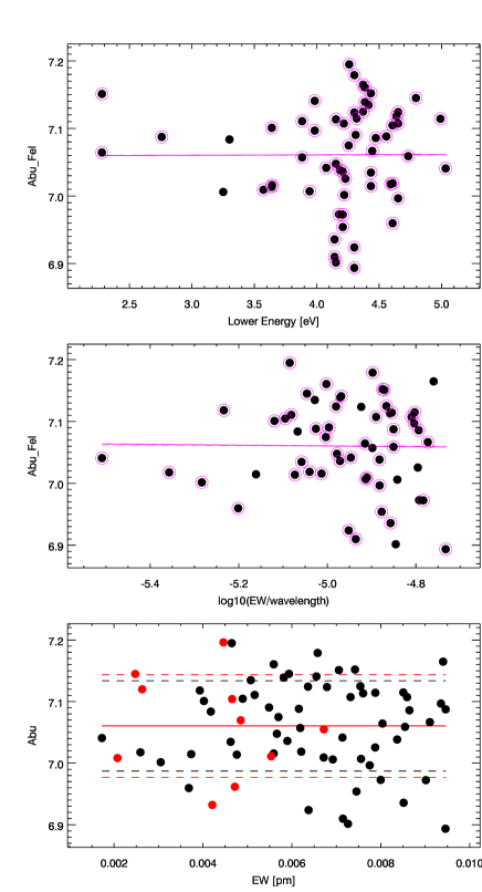
Figure 6: Same as in Fig. 5 for Arcturus. LEAS=0.0006 per eV. Fe i abundance vs. reduced EW slope $-6.4\leavevmode\nobreak\ 10^{-3}$. A(Fe i)$=7.06\leavevmode\nobreak\ \pm 0.07$, A(Fe ii)$=7.06\leavevmode\nobreak\ \pm 0.08$

Ca i lines as the ones measured in this example belong to a trace specie in such atmospheres, and are thus temperature sensitive but only weakly pressure sensitive. At the typical formation depths for weak lines ($\log($$\tau_{\mathrm{ross}}$$)$ roughly between –2 and 0) the three models are quite close in temperature. Pressure on the other hand is significantly different, but these lines are very weakly sensitive to it. Majority species lines (e.g. ionized element lines), or damped lines which have stronger pressure sensitivity, are likely to display stronger departures in this situation. As such, we suggest that users verify the abundances derived by MyGIsFOS for species which depart heavily from grid solar-scaled values. However, since significant differences might arise only for species strongly departing from solar abundance ratios, the detection of abundance anomalies through MyGIsFOS is to be considered robust, and only the exact amount of the abundance departure might be in need of verification.

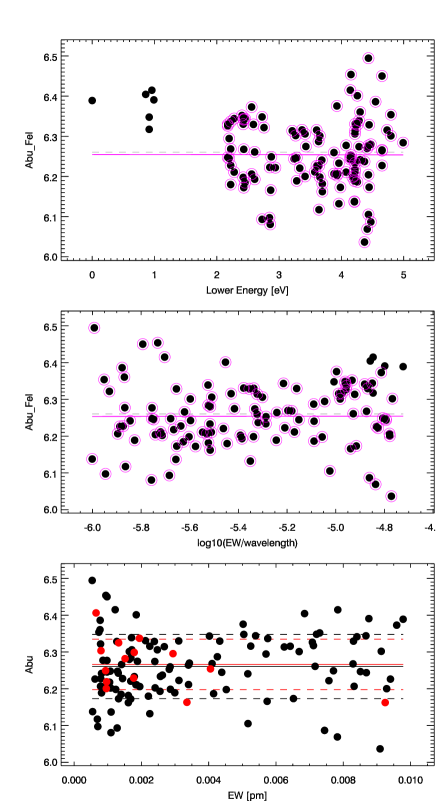
Figure 7: Same as in Fig. 5 for HD 126681. LEAS=-0.0002 per eV. Fe i abundance vs. reduced EW slope $8.0\leavevmode\nobreak\ 10^{-4}$. A(Fe i)$=6.26\leavevmode\nobreak\ \pm 0.09$, A(Fe ii)$=6.27\leavevmode\nobreak\ \pm 0.07$

6 Tests on reference stars

As an assessment of MyGIsFOS performance, we present in this section parameter determination and chemical analysis for a few representative stars. To reproduce typical data characteristics, very high S/N, high resolution spectra of five well studied stars have been noise-injected at typical “real world” values and analyzed using synthetic grids and feature lists appropriate for the four main broad spectra type: metal rich dwarf / subgiant stars (the Sun, see Sect. 6.1), metal poor dwarf / subgiants (HD 126681, Sect. 6.3, and HD 140283, Sect. 6.4), metal rich giants (Arcturus, Sect. 6.2), and metal poor giants (HD 26297, Sect. 6.5). Given the coverage provided by the available synthetic grid, the analysis has been performed using ranges roughly corresponding to UVES red 580nm setting, i.e. two frames covering 480 to 580nm, and 580 to 680nm. For each star, Table 3 and 4 report the final determined parameters, plus detailed abundances for a few chemical species, together with the number of lines used and line-to-line scatter, when more than one line was measured.

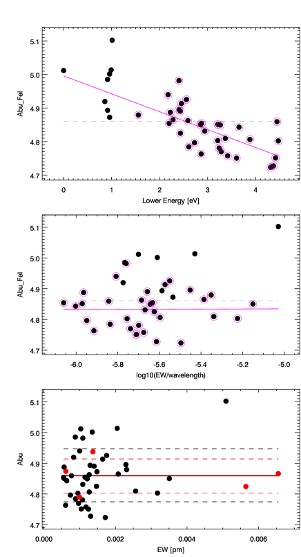
Figure 8: Same as in Fig. 5 for HD 140283 with temperature locked at $T_{\mathrm{eff}}$=5777 K. LEAS=-0.0534 per eV. Fe i abundance vs. reduced EW slope $2.3\leavevmode\nobreak\ 10^{-3}$. A(Fe i)$=4.86\leavevmode\nobreak\ \pm 0.09$, A(Fe ii)$=4.86\leavevmode\nobreak\ \pm 0.06$

6.1 The Sun

Diagnostic plots for the Sun are shown in Fig. 5, abundances listed in Table 3. A high S/N ($>$100) spectrum of Ceres was acquired (on 18/01/2008, UT 18:00:56, 900 s exposure) at SOPHIE@OHP (Bouchy & Sophie Team, 2006; Perruchot et al., 2008) in High Efficiency mode (resolution of 7.4 km s^-1), and was degraded to UVES-like sampling ($\sim$ 0.0025 nm per pixel) and noise-injected to S/N=50. Derived parameters ($T_{\mathrm{eff}}$=5794, $\log g$=4.55, V_turb=1.07 km s^-1, [$\alpha$/Fe]=0.05, [Fe/H]= –0.06 $\pm$0.059 over 84 Fe i features) are in excellent agreement with the Sun’s effective temperature and gravity ($T_{\mathrm{eff}}$=5777 K, $\log g$=4.44, Cox 2000). While the “canonical” value of the solar microturbulence for the full disk flux spectrum is 1.35 km s^-1 (Holweger et al., 1978) we note that an analysis conducted at lower resolution and based on an ATLAS 9 model derives 0.99 km s^-1 (Meléndez et al., 2012).

The difference from the established values are well within the dispersion of random S/N=50 noise injections, as presented below in 7.2.

6.2 Arcturus

The UVES POP (Bagnulo et al., 2003) spectrum for Arcturus derived with the Red UVES arm and 580nm setting was convolved with a gaussian to produce a spectrum with final resolution of 7.0 km s^-1, then noise-injected at S/N=50. Diagnostic plots are shown in Fig. 6, abundances listed in Table 3. The derived parameters ($T_{\mathrm{eff}}$=4293, $\log g$=1.84, V_turb=1.44 km s^-1, [$\alpha$/Fe]=0.19, [Fe/H]=–0.44 $\pm$0.073 over 59 Fe i features) are in excellent agreement with the values presented in Koch & McWilliam (2008) ($T_{\mathrm{eff}}$=4290, $\log g$=1.64, V_turb=1.54, [Fe/H]=–0.49).

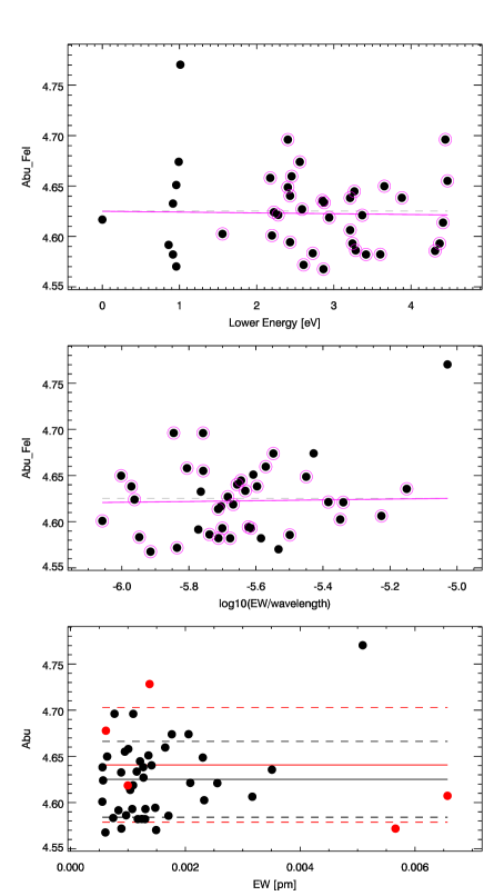
Figure 9: Same as in Fig. 5 for HD 140283 with temperature iterated. LEAS=–0.0008 per eV. Fe i abundance vs. reduced EW slope $4.3\leavevmode\nobreak\ 10^{-3}$. A(Fe i)$=4.63\leavevmode\nobreak\ \pm 0.04$, A(Fe ii)$=4.64\leavevmode\nobreak\ \pm 0.06$

6.3 HD 126681

HD 126681 is a good example of a moderately metal-poor dwarf star. A “traditional” fully spectroscopic parameter determination for this star, based on high resolution and S/N HARPS spectra is presented in Sousa et al. (2011). It is the very type of analysis MyGIsFOS aims to replicate, and leads to values of $T_{\mathrm{eff}}$=5561 $\pm$68 K, $\log g$=4.71 $\pm$0.1, V_turb=0.71 km s^-1, [Fe/H]=–1.14$\pm$0.06. Similarly to what we did for Arcturus, we have employed the UVES POP spectrum, degraded to a resolution of 7.4 km s^-1, and noise-injected to S/N=80. Diagnostic plots for the HD 126681 are shown in Fig. 7, abundances listed in Table 3. The derived values ($T_{\mathrm{eff}}$=5530, $\log g$=4.41, V_turb=0.50, [$\alpha$/Fe]=0.38, [Fe/H]=–1.24 $\pm$0.087 over 116 features) are in very good agreement with the above stated values. The [Fe/H] discrepancy is a bit higher than expected, our metallicity being lower by 0.10 dex. It is worth noting how a change upwards of Fe i abundance alone would lead ionization equilibrium to settle to a somewhat higher gravity, as found by Sousa et al. (2011). We have not further investigated this slight discrepancy, which can stem from a number of differences, including differences in Fe i line data, or the fact that Sousa et al. (2011) use a model grid with a different set of opacities and the overshooting option switched on. The difference between overshooting and non-overshooting ATLAS models can account for a 0.1  dex difference.

6.4 HD 140283

HD 140283 is the prototypical metal-poor star (Chamberlain & Aller, 1951), very often employed as a reference for stars in this metallicity range (recently, Hosford et al., 2009; Hosford et al., 2010; Casagrande et al., 2010; Bergemann et al., 2012, among others). Recently its distance has been estimated through HST observations (Bond et al., 2013), allowing to estimate an age of 14.46 $\pm 0.8$ Gyr. Hosford et al. (2009) noticed how attempting to constrain ionization and excitation equilibrium together led to a relatively low temperature (5573 K) and consequently to a low gravity incompatible with the known Hipparcos-based luminosity. The InfraRed Flux Method (IRFM) based temperature (5691  K Alonso, 5755 K González Hernández & Bonifacio 2009, 5777 K Casagrande et al. 2010) delivers a more satisfactory ionization equilibrium when gravity is derived from the Hipparcos luminosity, but at the expense of inducing a sizeable LEAS (see Tables 2, 3 and figure 11 in Bergemann et al., 2012). According to Hosford et al. (2010), treating the line transfer for Fe i lines in NLTE solves this discrepancy and provides an excitation temperature of 5838 K, in reasonable agreement with the IRFM temperatures. Bergemann et al. (2012) disagree with this finding. What is relevant in the present context is that solving for both excitation and ionization equilibria of iron in LTE for HD 140283 leads to low temperature and gravity and on this issue Hosford et al. (2009) and Bergemann et al. (2012) agree.

We employed the UVES POP red arm 580 nm spectra, without adding instrumental broadening or injecting noise: given the high resolution, stellar rotation and macroturbulence might require a broadening of the grid above what necessary to take into account the instrumental resolution. We adjusted the grid broadening until we obtained satisfactory fits on several isolated lines. The final grid broadening employed was 5.5 km s^-1. We ran MyGIsFOS on this star twice, once leaving the code free to constrain all the parameters, and once locking $T_{\mathrm{eff}}$ to 5777 K. Diagnostic plots for the HD 140283 are shown in Fig. 8 and 9, abundances listed in Table 4. When leaving MyGIsFOS free to set $T_{\mathrm{eff}}$, it falls to 5506 K, resonably close to the excitation temperature found by Hosford et al. (2009) driving also down [Fe/H] to –2.87, and $\log g$ to 2.86. When fixing $T_{\mathrm{eff}}$ at 5777 K, instead, the derived gravity (3.32) is in reasonable agreement with the Hipparcos value (3.73), and V_turb is also very close to the value derived in Bergemann et al. (2012) in the LTE case (1.22 km s^-1 vs. 1.27). However, the metallicity we derive is lower by about 0.22 dex ([Fe/H]=–2.64 vs. –2.42).

6.5 HD 26297

HD 26297 is a moderately metal-poor giant star. A spectroscopic abundance analysis similar to the one MyGIsFOS performs is presented in Fulbright (2000) ($T_{\mathrm{eff}}$=4500 K, $\log g$=1.2, [Fe/H]=–1.72), while Gratton et al. (2000) obtains similar values ($T_{\mathrm{eff}}$=4450 K, $\log g$=1.18, [Fe/H]=–1.68, V_turb=1.62 km s^-1) but deriving temperature and gravity from photometric calibrations (Fe ionization equilibrium is very well satisfied for this star). A more recent analysis, presented in Prugniel et al. (2011), uses instead a $\chi^{2}$ minimization algorithm to fit the target spectrum agains the empirical ELODIE library (see Wu et al., 2011), and delivers $T_{\mathrm{eff}}$=4479 K, $\log g$=1.05, [Fe/H]=–1.78.

We downloaded archival UVES red 580 spectra for HD 26297 (taken on 20/11/2004, 01:39:42 UT, prog. id 074.B-0639). The data were taken with slit width of 0.9” and have a good S/N ($>$100). No additional noise was injected. They were analyzed by broadening the synthetic grid to 7.5 km s^-1. Diagnostic plots are shown in Fig. 10, abundances listed in Table 4. We derive $T_{\mathrm{eff}}$=4458, $\log g$=1.06, V_turb=1.76, [$\alpha$/Fe]=0.36, [Fe/H]=$-1.83\pm$0.07 over 83 Fe i lines, in excellent agreement with all the cited sources.

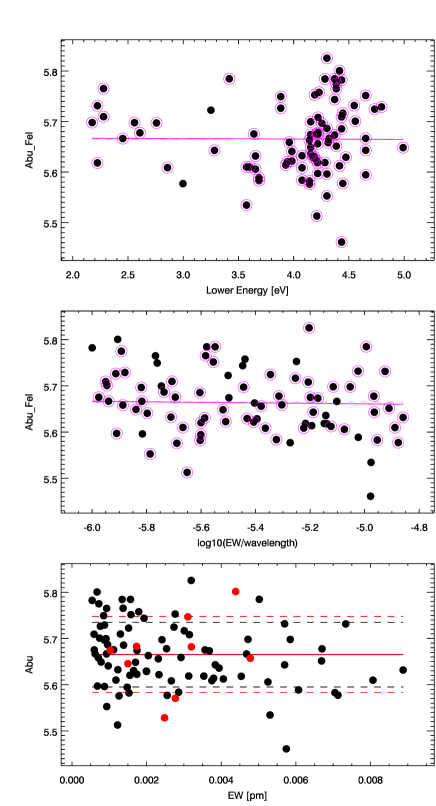
Figure 10: Same as in Fig. 5 for HD 26297. LEAS=0.0009 per eV. Fe i abundance vs. reduced EW slope $-5.6\leavevmode\nobreak\ 10^{-3}$. A(Fe i)$=5.67\leavevmode\nobreak\ \pm 0.07$, A(Fe ii)$=5.67\leavevmode\nobreak\ \pm 0.08$

7 Montecarlo simulations

Table 4: Determined abundances for HD 140283 with fixed and free $T_{\mathrm{eff}}$, and HD 26297.

	HD 140283(a): $T_{\mathrm{eff}}$=5777, $\log g$=3.32,			HD 140283(b): $T_{\mathrm{eff}}$=5506 $\log g$=2.85			HD 26297 $T_{\mathrm{eff}}$=4458, $\log g$=1.06,
	Vturb=1.22, [$\alpha$/Fe]=0.26			Vturb=1.33, [$\alpha$/Fe]=0.35			Vturb=1.76, [$\alpha$/Fe]=0.36
	Number of	[Fe/H] or	$\sigma$	Number of	[Fe/H] or	$\sigma$	Number of	[Fe/H] or	$\sigma$
	features	[X/Fe](c)		features	[X/Fe](c)		features	[X/Fe](c)
Fe i	41	–2.64	0.086	41	–2.87	0.041	85	–1.83	0.070
Fe ii	5	–2.64	0.056	5	–2.86	0.062	9	–1.83	0.082
Na i	–	–	–	–	–	–	3	–0.41	0.102
Mg i	1	0.49	–	1	0.57	–	1	0.53	–
Al i	–	–	–	–	–	–	1	–0.06	–
Si i	–	–	–	–	–	–	6	0.26	0.077
Ca i	6	0.26	0.093	6	0.35	0.044	9	0.28	0.075
Ti i	4	0.40	0.087	4	0.33	0.043	16	0.22	0.097
Ti ii	4	0.28	0.182	4	0.32	0.261	5	0.23	0.356
Ni i	2	0.11	0.243	2	0.11	0.155	10	–0.11	0.101

One attractive possibility opened by fully automated abundance analysis codes such as MyGIsFOS is to comprehensively assess the error budget by means of Montecarlo simulations, since large number of test “events” can be processed through the code in very little time.

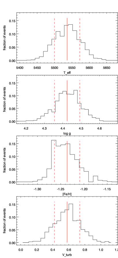
Figure 11: Histograms of MyGIsFOS parameter determination output in a Montecarlo simulation of 1000-events noise injection at S/N=80 on a spectrum of HD 126681. Top to bottom: determined $T_{\mathrm{eff}}$ (mean and $\sigma$, continuous and dashed red lines, respectively, all values in Table 5), $\log g$, [Fe/H], V_turb.

7.1 Impact of S/N ratio: internal errors.

To assess the size of MyGIsFOS internal errors, as well as the extent to which the code is affected by spectrum noise, we have employed a synthetic spectrum extracted from the MPD grid at $T_{\mathrm{eff}}$=5400 K, $\log g$=4.5, V_turb=1.0 kms^-1, [Fe/H]=-1.0, [$\alpha$/Fe]=+0.4, and have processed it to MyGIsFOS after broadening it to a resolution of 7.4 kms^-1, and resampling it to typical UVES pixel size. We have first processed it without injecting noise to ensure the absence of systematics, and subsequently produced 1000 independent Poisson noise realizations at S/N=80, 50, 20, for a total of 3000 noise realizations, which were fed to MyGIsFOS, which was set to derive $T_{\mathrm{eff}}$, $\log g$, V_turb, [Fe/H], and [$\alpha$/Fe]. The results of the noiseless test, as well as derived average values and $1\sigma$ dispersions for the noise-injection montecarlo tests are listed in Table 5.

It is worth noticing how the errors displayed by MyGIsFOS in the synthetic test match closely the ones in the case of HD126681. One might have expected that feeding MyGIsFOS a spectrum of the same grid used for the analysis would ahve led to the code “snapping” on the right parameters, leading to lower-than-realistic errors. However, MyGIsFOS only compares the grid and the observed on a line-by-line basis, and parameters are all derived by indirect methods. Moreover, the initial temperature scan is purposefully performed at steps different from the grid step, so that comparison is always performed away from gridpoints, removing any “grid snapping” effect.

7.2 Impact of S/N ratio: HD126681

To assess the impact of external error sources we have repeated the above described test on the very high S/N spectrum of HD126681 described in 6.3. Again, 1000 independent Poisson noise realization were produced for S/N=89, 50, 20 each. Derived average values and $1\sigma$ dispersion sare listed in Table 5, the histograms of the parameters are presented in Fig. 11 through 13.

MyGIsFOS is not allowed to try indefinitely to bring stellar parameters to convergence. After a set number of “cycles” it stops, declares the star non-converging and passes to the next one. It is worth noticing here that, while S/N=80 and 50 Montecarlo tests had every single star reaching satisfactory convergence, in the S/N=20 case convergence was reached in 943 over 1000 realizations (a failure rate of 5.7%). Unsurprisingly, at such low S/N the difficulty of measuring weak lines, needed especially for V_turb determination, begins to take its toll. Moreover, 138 converging stars end up with V_turb=0, a clearly visible peak in Fig. 13. This is just the natural consequence of a V_turb distribution centered at 0.39 km s^-1 with a $\sigma$ of 0.28: in a relevant number of stars the specific set of Fe i lines used would push for a negative V_turb, which MyGIsFOS forbids as unphysical.

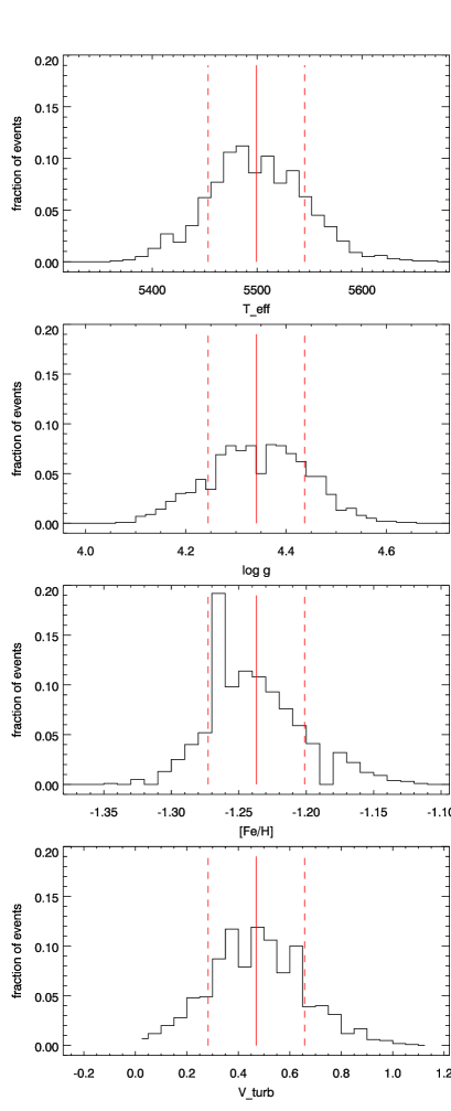
Figure 12: As in Fig. 11 but now with S/N=50.

It is to be remarked that the presented test is a simplified one and the resulting uncertainties are possibly somewhat underestimated. In particular, the injection of Poisson noise is a somewhat “optimistic” way to simulate real observed spectrum noise degradation, since it lacks a number of realistic outstanding defects real, low S/N spectra present (cosmic ray hits, poor order tracing in low S/N cases, increased noise at order merging points…). Also, noise has been injected here to produce constant S/N through the range, which is not the case in practice, often with lower S/N in the bluer part of the range, where most of the atomic lines are concentrated.

7.3 Impact of pre-determined parameters: photometric $T_{\mathrm{eff}}$

Most abundance analysis works typically assess the impact of errors on atmospheric parameters on derived abundances by assuming said errors are independent. This is often performed by picking a representative star in the sample, and repeating the abundance determination by varying one parameter at the time by an amount considered to be the typical uncertainty on that parameter. This quick way of estimating parameter uncertainties is, however, conceptually flawed in the sense that atmospheric parameters correlate in a fashion that is, ultimately, dependent on the specific way they are derived. For instance, if gravity is determined from Fe i-Fe ii ionization equilibrium, varying $T_{\mathrm{eff}}$ by 150 K will lead to a different gravity too: repeating the analysis with a different temperature but the same gravity will not be representative of which effect a 150 K $T_{\mathrm{eff}}$ error would have in a “real world” case.

A fairly common case in which such issue is of importance is the one in which effective temperatures are derived independently from the spectra, e.g. from photometry. In this case, errors in the other parameters will cascade from whatever error is made in $T_{\mathrm{eff}}$, in a systematic way. MyGIsFOS allows to estimate the effect through a Montecarlo test set. We have again constructed a 1000-events test set but, differently from what done in 7.2, we have now analyzed one single realization of S/N=80 noise injection, starting from the same HD 126681 high-S/N spectrum. The test set has been constructed now by drawing 1000 $T_{\mathrm{eff}}$ values from a gaussian distribution centered at 5552 K and with a $\sigma$ of 150 K, and having MyGIsFOS run with fixed $T_{\mathrm{eff}}$. The resulting histograms are shown in Fig. 14, the resulting distributions in the other parameters and metallicity are again given in Table 5. Although we do not present it here, a more detailed species-by-species error estimate is of course possible, thus allowing to properly assess parameter-related uncertainties on any abundance. The same kind of procedure is of course possible when more than one parameter is kept fixed (e.g. the case of photometric $T_{\mathrm{eff}}$ and $\log g$ derived from isochrones).

8 Performance, system requirements, and availability

MyGIsFOS is written in Fortran 90 with Intel extensions. So far it has been compiled and run under Linux and Mac OS X.

Table 5: Average parameter values and $1\sigma$ intervals for the Montecarlo tests described in 7. In order, the result of the analysis of the noiseless synthetic spectrum, of the three 1000 noise realization runs on the synthetic (for both see 7.1), of the three 1000 noise realization runs on HD126681, and of the “photometric $T_{\mathrm{eff}}$” run on HD126681 (for both see 7.2). In the last row, $T_{\mathrm{eff}}$ and its $\sigma$ are in boldface to indicate they are not results, but the fixed input $T_{\mathrm{eff}}$ distribution

Test type	$T_{\mathrm{eff}}$	$\sigma$	$\log g$	$\sigma$	[Fe/H]	$\sigma$	Vturb	$\sigma$
	K		$cm\leavevmode\nobreak\ s^{-1}$				$km\leavevmode\nobreak\ s^{-1}$
synthetic noiseless	5403	–	4.51	–	–1.00	–	0.97	–
synthetic S/N=80	5409	31	4.51	0.06	–1.01	0.02	1.05	0.07
synthetic S/N=50	5419	36	4.54	0.08	–1.00	0.03	1.04	0.09
synthetic S/N=20	5461	80	4.57	0.18	–0.95	0.06	0.94	0.22
HD126681 S/N=80	5536	36	4.42	0.07	–1.24	0.03	0.58	0.16
HD126681 S/N=50	5499	46	4.34	0.10	–1.24	0.03	0.47	0.19
HD126681 S/N=20	5422	87	4.10	0.20	–1.22	0.07	0.39	0.28
HD126681 fixed $T_{\mathrm{eff}}$, S/N=80	5552	150	4.43	0.29	–1.24	0.12	0.77	0.22

MyGIsFOS synthetic grids can grow to significant sizes when covering large spectral ranges and a large parameter space. As an example we can consider the grid employed in Sections 6.3, 6.4, and 7, intended to handle UVES RED 580 spectra of metal poor, cool turn-off and dwarf stars. It is composed of two frames (460 to 590, and 560 to 690 nm) synthesized (from ATLAS12 atmosphere models and by using SYNTHE, see Sbordone et al., 2004; Castelli, 2005; Kurucz, 2005; Sbordone, 2005) with velocity-equispaced, R=300000 sampling. The spectra are computed for 3840 parameter values. The binary packaged grid has a size of about 2.2GB. The size of the grid sets the main resource requirement, since the grid is twice resident in memory (the master copy read in at the beginning of the run, and the one, smaller, resampled to the observed pixels of the star being currently processed). Also, grid resampling at observed spectrum pixel wavelengths is usually the longest operation in the processing of a star. For both these reasons, it is always advisable to use the smallest desirable grid both in terms of parameter space and spectrum coverage.

Figure 13: As in Fig. 11 but now with S/N=20.

As a benchmarking and resource consumption reference we use typical values for one of the S/N Montecarlo runs described in 7.2. The run was executed on a quad-core Intel Xeon E31245, 3.3GHz, machine with 11.6 GB of RAM, running openSUSE 12.3 with 3.7.10 64bit kernel. Employing the grid described above in this same section, peak MyGIsFOS memory consumption was 3.5 GB, with an average processing time per star (over 1000 stars) of 119s, running on a single core. These values are to be considered upper limits. In the described case the resampling of $\sim 74700$ synthetic grid “pixels” over the $\sim$71000 observed ones takes somewhat more of 50% of the total per-star processing time, almost all the rest being taken by the $\sim$280 parameter-finding iterations needed to determine $T_{\mathrm{eff}}$, $\log g$  V_turb, [Fe/H], and [$\alpha$/Fe]. At the other extreme, determining only [Fe/H], [$\alpha$/Fe], and detailed abundances at pre-defined atmospheric parameters on data constituted by two FLAMES high-resolution settings takes less than 10 seconds per star, thanks equally to the lack of parameter iteration and to the small number of pixels over which grid resampling should be performed.

For the time being, MyGIsFOS is available on a collaboration basis only. A website has been set up Eto make detailed code documentation available to interested parties, so that they can assess whether it can be of use to them before contacting us.

Figure 14: Histograms of MyGIsFOS parameter determination output in a 1000-events Montecarlo simulation with fixed $T_{\mathrm{eff}}$, on a S/N=80 spectrum of HD 126681. Panels as in Fig. 11.

9 Conclusions

We have presented MyGIsFOS, an automatic code for the determination of atmospheric parameters and detailed chemical abundances in cool stars. Replicating as closely as possible a “traditional” manual abundance analysis technique for this type of stars, MyGIsFOS derives results directly and quickly comparable with well known analysis techniques. Currently, MyGIsFOS has been employed on the same type of data that are best suited for the manual techniques it replicates, i.e. those characterized by high-resolution and/or broad spectral coverage, such as the ones delivered by UVES, X-Shooter, HARPS, Sophie (Caffau et al., 2011; Bonifacio et al., 2012; Caffau et al., 2012; Caffau et al., 2013; Duffau et al., 2014). Its very fast operation (2 minutes or less per star on a mainstream personal computer) is convenient in a number of circumstances.

• When analyzing large datasets of (broadly) homogeneous data in the context of large scale spectroscopic surveys such as for instance the Gaia-ESO Public Survey (UVES data, see Gilmore et al., 2012).

• When screening large amounts of low-intermediate resolution spectra for interesting candidates to be followed up. While MyGIsFOS delivers its full capability for high-resolution (R$\geq$ 25000), large spectral coverage data, it can be effectively used to derive global metallicity from low resolution spectra, once parameters can be inferred from other sources. In this context Abbo (Bonifacio & Caffau, 2003), the code MyGIsFOS has been derived from, has been employed to select extremely metal poor Turn-Off candidates from low-resolution SDSS-SEGUE (York et al., 2000; Yanny et al., 2009) spectra, which were then followed up at high resolution, showing a remarkable selection success rate (e. g. Caffau et al., 2012; Bonifacio et al., 2012; Caffau et al., 2011), and MyGIsFOS is currently used in the same capacity in the context of the TOPoS ESO Large Program (Turn-Off Primordial Stars, Caffau et al., 2013).

• When extending pre-existing literature datasets with new data: when adding new stars to pre-existing samples of abundances derived in previous papers, it is usually impractical to re-analize the existing corpus of data, so homogeneity issues arise because of differences e.g. in atmosphere modeling, or atomic data choices. The very fast processing of MyGIsFOS allows, on the other hand, to repeat the analysis of the whole sample every time in a fully homogeneous way. As a matter of fact, fully parallel analyses can be conducted e. g. with different atmospheric parameter choices, with practically no time penalty.

• To consistently tackle error propagation through the analysis pipeline by means of Montecarlo simulations, as presented in Sect. 7.3 for photometric effective temperatures. This is almost never done due to the very high time cost it would usually imply, but it would be of great importance since errors in atmospheric parameters and abundances are in general strongly correlated, and method dependent.