Random Generation of
Nondeterministic Finite-State Tree Automata

Abstract

Algorithms for (nondeterministic) finite-state tree automata (FTAs) are often tested on random FTAs, in which all internal transitions are equiprobable. The run-time results obtained in this manner are usually overly optimistic as most such generated random FTAs are trivial in the sense that the number of states of an equivalent minimal deterministic FTA is extremely small. It is demonstrated that nontrivial random FTAs are obtained only for a narrow band of transition probabilities. Moreover, an analytic analysis yields a formula to approximate the transition probability that yields the most complex random FTAs, which should be used in experiments.

1 Introduction

Nondeterministic finite-state tree automata (FTAs) play a major role in several areas of natural language processing. For example, the Berkeley parser [11] uses a (weighted) FTA as do syntax-based approaches to statistical machine translation. Toolkits [10, 8] for FTAs allow users to easily run experiments. However, algorithms like determinization typically cannot be tested on real-world examples (like the FTA of the Berkeley parser) due to their complexity. In such cases, the inputs are often random FTAs, which are typically created by fixing densities, which are the probabilities that any given potential transition (of a certain group) is indeed a transition of the generated FTA (see [13] and [9] for the generation of random finite-state string automata).

It is known [3] that for string automata most random automata are trivial in the sense that the equivalent minimal deterministic finite-state string automaton is extremely small. Here, we observe the same effect for FTAs, which means that testing algorithms on random FTAs also has to be done carefully to avoid vastly underestimating their actual run-time. To simplify such experiments and to make them more representative we provide both empirical and analytic evidence for the nontrivial (difficult) cases. In the empirical evaluation we create many random FTAs with a given number $n$ of (useful) states using a given transition density $d$. We then determinize and minimize them, and we record the number of states of the resulting canonical FTA (i.e., the equivalent minimal deterministic FTA). As expected, outside a narrow density band the randomly generated FTAs yield very small canonical FTA, which means that they are in a sense trivial. It can be observed that if the density is above the upper limit of the band, then the FTAs accept almost everything, whereas FTAs with densities below the lower limit accept almost nothing. This observation also justifies calling them trivial.

In the analytic evaluation, given a number $n$ of states, we compute densities $d(n)$, for which we expect the most difficult FTAs. Looking at the empirical results, the formula predicts the narrow density band belonging to complex random FTAs very well. Consequently, we promote experiments with random FTAs that use exactly these predicted densities in order to avoid experiments with (only) trivial FTAs. Finally, we discuss how parameter changes affect our results. For example, adding another binary input symbol does not move the interesting narrow density band, but it generally does increase the sizes of the obtained canonical FTA. Moreover, it shows that whenever we obtain large deterministic FTA after determinization (i.e., before minimization), then the corresponding canonical FTA are also large (i.e., after minimization). This demonstrates that our implementation of determinization is rather efficient.

2 Finite tree automata

The power set of a set $S$ is $\mathcal{P}(S)=\{S^{\prime}\mid S^{\prime}\subseteq S\}$. The set of nonnegative integers is denoted by ${\rm Nature}$. An alphabet is simply a finite set of symbols. A ranked alphabet $(\Sigma,\mathord{\operatorname{rk}})$ consists of an alphabet $\Sigma$ and a mapping $\mathord{\operatorname{rk}}\colon\Sigma\to{\rm Nature}$, which assigns a rank to each symbol. For every $k\in{\rm Nature}$, we let $\Sigma_{\_}k=\{\sigma\in\Sigma\mid\operatorname{rk}(\sigma)=k\}$ be the set of symbols of rank $k$. We also write $\sigma^{(k)}$ to indicate that the symbol $\sigma$ has rank $\operatorname{rk}(\sigma)=k$. To keep the presentation simple, we typically write just $\Sigma$ for the ranked alphabet $(\Sigma,\mathord{\operatorname{rk}})$ and assume that the ranking ‘$\mathord{\operatorname{rk}}$’ is clear from the context. Moreover, we often drop obvious universal quantifications like ‘$k\in{\rm Nature}$’ in expressions like ‘for all $k\in{\rm Nature}$ and $\sigma\in\Sigma_{\_}k$’. Our trees have node labels taken from a ranked alphabet $\Sigma$ and leaves can also be labeled by elements of a finite set $Q$. The rank of a symbol $\sigma\in\Sigma$ determines the number of direct children of all nodes labeled $\sigma$. Given a set $T$, we write $\Sigma(T)$ for the set $\{\sigma(t_{1},\dotsc,t_{k})\mid\sigma\in\Sigma_{\_}k,t_{1},\dotsc,t_{k}\in T\}$. The set $T_{\_}\Sigma(Q)$ of $\Sigma$-trees indexed by $Q$ is defined as the smallest set $T$ such that $\Sigma(T)\cup Q\subseteq T$. We write $T_{\_}\Sigma$ for $T_{\_}\Sigma(\emptyset)$.

Next, we recall finite-state tree automata [5, 6] and the required standard constructions. In general, finite-state tree automata (FTAs) offer an efficient representation of the regular tree languages. We distinguish a (bottom-up) deterministic variant called deterministic FTA, which will be used in our size measurements. A finite-state tree automaton (FTA) is a system $(Q,\Sigma,F,P)$, where (i) $Q$ is a finite set of states, (ii) $\Sigma$ is a ranked alphabet of input symbols, (iii) $F\subseteq Q$ is a set of final states, and (iv) $P\subseteq\Sigma(Q)\times Q$ is a finite set of transitions. It is deterministic if for every $t\in\Sigma(Q)$ there exists at most one $q\in Q$ such that $(t,q)\in P$. We often write a transition $(t,q)\in\Sigma(Q)\times Q$ as $t\to q$. The size of the FTA $M=(Q,\Sigma,F,P)$ is $\lvert M\rvert=\lvert Q\rvert$. This is arguably a crude measure for the ‘size’, but it will mostly be used for deterministic FTAs, where it is commonly used.

Example 1.

As illustration we consider the FTA $M_{\_}{\text{ex}}=(\{0,1,2,3\},\Sigma,\{3\},P)$, where $\Sigma=\{\sigma^{(2)},\alpha^{(0)}\}$ and $P$ contains the following transitions. Clearly, this FTA is not deterministic.

$$\alpha \to 0 \alpha \to 2 \sigma(0,0) \to 1 \sigma(1,0) \to 1 \sigma(1,2) \to 3 \sigma(1,3) \to 3$$

In the following, let $M=(Q,\Sigma,F,P)$ be an FTA. For every $\sigma\in\Sigma_{\_}k$, let $\overline{\sigma}\colon\mathcal{P}(Q)^{k}\to\mathcal{P}(Q)$ be such that $\overline{\sigma}(Q_{1},\dotsc,Q_{k})=\{q\in Q\mid\forall 1\leq i\leq k,\,\exists q_{\_}i\in Q_{\_}i\colon\sigma(q_{1},\dotsc,q_{k})\to q\in P\}$ for all $Q_{1},\dotsc,Q_{k}\subseteq Q$. Next, we define the action of the transitions on a tree $t\in T_{\_}\Sigma(Q)$. Let $P\colon T_{\_}\Sigma(Q)\to\mathcal{P}(Q)$ be such that $P(q)=\{q\}$ for every $q\in Q$ and $P(\sigma(t_{1},\dotsc,t_{k}))=\overline{\sigma}(P(t_{\_}1),\dotsc,P(t_{\_}k))$ for every $\sigma\in\Sigma_{\_}k$ and $t_{1},\dotsc,t_{k}\in T_{\_}\Sigma$. The FTA $M$ accepts the tree language $L(M)$, which is given by $L(M)=\{t\in T_{\_}\Sigma\mid P(t)\cap F\neq\emptyset\}$. Two FTAs $M_{\_}1$ and $M_{\_}2$ are equivalent if $L(M_{\_}1)=L(M_{\_}2)$. For example, for the FTA of Example 1 we have $P(\alpha)=\{0,2\}$ and $P(\sigma(\alpha,\alpha))=\{1\}$. Moreover, $\sigma(\sigma(\sigma(\alpha,\alpha),\alpha),\alpha)\in L(M_{\_}{\text{ex}})$. For our experiments, we generate a random FTA, then determinize it and compute the number of states of the canonical FTA, which the equivalent minimal deterministic FTA. For an FTA $M=(Q,\Sigma,F,P)$, we construct the deterministic FTA $\mathcal{P}(M)=(\mathcal{P}(Q),\Sigma,F^{\prime},P^{\prime})$ such that $F^{\prime}=\{Q^{\prime}\subseteq Q\mid Q^{\prime}\cap F\neq\emptyset\}$ and

$$P^{\prime}=\{\sigma(Q_{1},\dotsc,Q_{k})\to\overline{\sigma}(Q_{1},\dotsc,Q_{k})\mid\sigma\in\Sigma_{\_}k,Q_{1},\dotsc,Q_{k}\subseteq Q\}\enspace.$$

Theorem 2 (see [4, Theorem 1.10]).

$\mathcal{P}(M)$ is a deterministic FTA that is equivalent to $M$.

Example 3.

For the FTA $M_{\_}{\text{ex}}$ of Example 1 an equivalent deterministic FTA is $\mathcal{P}(M_{\_}{\text{ex}})$, which is given by $\mathcal{P}(M_{\_}{\text{ex}})=(\mathcal{P}(Q),\Sigma,F^{\prime},P^{\prime})$ with $F^{\prime}=\{3,13,23,123\}$ and $P^{\prime}$ contains the (non-trivial) transitions

$$\alpha \to 02 \sigma(02,02) \to 1 \sigma(1,02) \to 13 \sigma(13,02) \to 13 \sigma(1,13) \to 3 \sigma(1,3) \to 3\enspace.$$

A deterministic FTA is minimal if there is no strictly smaller equivalent deterministic FTA. For example, the deterministic FTA in Example 3 is minimal. It is known [2] that for every deterministic FTA we can compute an equivalent minimal deterministic FTA, called the canonical FTA.

3 Random generation of FTAs

First, we describe how we generate random FTAs. We closely follow the random generation outlined in [13], augmented by density parameters $d_{\_}2$ and $d_{\_}0$, which is similar to the setup of [9]. Both methods [13, 9] are discussed in [3], where they are applied to finite-state string automata [12]. For an event $E$, let $\pi(E)$ be the probability of $E$. To keep the presentation simple, we assume that the ranked alphabet $\Sigma$ of input symbols is binary (i.e., $\Sigma=\Sigma_{\_}2\cup\Sigma_{\_}0$). Note that all regular tree languages [5, 6] can be encoded using a binary ranked alphabet. In order to randomly generate an FTA $M=(Q,\Sigma,F,P)$ with $n=\lvert Q\rvert$ states and binary and nullary transition densities $d_{\_}2$ and $d_{\_}0$, each transition (incl. the target state) is a random variable and each state is a random variable representing whether it is final or not. More precisely, we use the following approach:

• $Q=\{1,\dotsc,n\}$,

• $\pi(q\in F)=\tfrac{1}{2}$ for all $q\in Q$ (i.e., for each state $q$ the probability that it is final is $\tfrac{1}{2}$),

• $\pi(\alpha\to q\in P)=d_{\_}0$ for all nullary $\alpha\in\Sigma_{\_}0$ and $q\in Q$, and

• $\pi(\sigma(q_{\_}1,q_{\_}2)\to q\in P)=d_{\_}2$ for all binary symbols $\sigma\in\Sigma_{\_}2$ and all states $q_{\_}1,q_{\_}2,q\in Q$.

If the such created FTA is not trim, then we start over and generate a new FTA. Thus, all our randomly generated FTAs indeed have $n$ useful states.

$n$	$d_{\_}2$	$d^{\prime}_{\_}2$	conf. interval		$n$	$d_{\_}2$	$d^{\prime}_{\_}2$	conf. interval
2	.6364	.6264	[.5769,.6804]		8	.0431	.0408	[.0317,.0526]
3	.2965	.2570	[.2091,.3159]		9	.0341	.0342	[.0272,.0430]
4	.1696	.1334	[.1024,.1737]		10	.0276	.0282	[.0231,.0343]
5	.1094	.0855	[.0642,.1138]		11	.0228	.0251	[.0208,.0303]
6	.0763	.0635	[.0475,.0848]		12	.0192	.0212	[.0182,.0248]
7	.0562	.0501	[.0380,.0662]		13	.0164	.0189	[.0162,.0219]

Table 1: Expected density $d_{\_}2$ (see Theorem 4) and observed density $d^{\prime}_{\_}2$ (see Section 5) for the most complex FTAs in Setting (A). We also report confidence intervals for the confidence level $p>.95$.

4 Analytic analysis

In this section, we present a short analytic analysis and compute densities, for which we expect the randomly generated FTAs to be non-trivial. More precisely, we estimate for which densities the determinization (and subsequent minimization) returns the largest canonical FTAs. It is known from the generation of random finite-state string automata [3] that the largest deterministic automata are obtained during determinization if each state $q\in Q$ occurs with probability $\tfrac{1}{2}$ in the transition target of a transition, in which the source states are selected uniformly at random. This observation was empirically confirmed multiple times by independent research groups [9, 13, 3]. In addition, all transition target states are equiprobable for input states that are drawn uniformly at random. This latter observation supports the optimality claim by arguments from information theory because if all target states of a transition are equiprobable, then the entropy of the transition is maximal. While these facts support our hypothesis (and subsequent conclusions), we also rely on an empirical evaluation in Section 5 to validate it.

The determinization (see Section 2) constructs the state set ${\cal P}(Q)$. Let ${\cal P}(M)=({\cal P}(Q),\Sigma,F^{\prime},P^{\prime})$ be the deterministic FTA given the random FTA $M$ with $n=\lvert Q\rvert$. According to our intuition, the probability that a state $Q^{\prime}\in{\cal P}(Q)$ is the transition target of a given transition $\sigma(Q_{\_}1,Q_{\_}2)$, where $Q_{\_}1$ and $Q_{\_}2$ are uniformly selected at random from ${\cal P}(Q)$, should be $2^{-n}$ [i.e., $\pi(\sigma(Q_{\_}1,Q_{\_}2)\to Q^{\prime}\in P^{\prime})=2^{-n}$]. Thus, in particular, each given state $q\in Q$ is in the (real) successor state $Q^{\prime\prime}$ of the given transition $\sigma(Q_{\_}1,Q_{\_}2)$ with probability $\tfrac{1}{2}$ [i.e., $\pi(q\in Q^{\prime\prime})=\tfrac{1}{2}$]. Given $\sigma\in\Sigma_{\_}2$ and $q\in Q$, let $\pi_{\_}{\sigma,q}=\pi(q\in Q^{\prime\prime})$, where $Q_{\_}1$ and $Q_{\_}2$ are uniformly selected at random from ${\cal P}(Q)$ and $Q^{\prime\prime}=\overline{\sigma}(Q_{\_}1,Q_{\_}2)$. Similarly, given $\alpha\in\Sigma_{\_}0$ and $q\in Q$, let $\pi_{\_}{\alpha,q}=\pi(q\in\overline{\alpha})$. It is easily seen that $\pi_{\_}{\sigma,q}=\pi_{\_}{\sigma^{\prime},q^{\prime}}$ for all $\sigma,\sigma^{\prime}\in\Sigma_{\_}2$ and $q,q^{\prime}\in Q$ because in our generation model all $\sigma$-transitions in $M$ with $\sigma\in\Sigma_{\_}2$ are equiprobable. Thus, we simply write $\pi_{\_}2$ instead of $\pi_{\_}{\sigma,q}$. The same property holds for nullary symbols, so we henceforth write $\pi_{\_}0$ for $\pi_{\_}{\alpha,q}$. Moreover, as in the previous section, let $n$ be the number of states of the original random FTA, and let $d_{\_}2$ and $d_{\_}0$ be the transition densities of it. For $n=1$ the presented intuition cannot be met.

Theorem 4.

Let $n>1$. If $d_{\_}2=4(1-\sqrt[n^{2}]{.5})$ and $d_{\_}0=\tfrac{1}{2}$, then $\pi_{\_}2=\pi_{\_}0=\tfrac{1}{2}$.

Proof.

We start with $\pi_{\_}0$. Let $\alpha\in\Sigma_{\_}0$ and $q\in Q$. Then $\pi(q\in\overline{\alpha})=\pi(\alpha\to q\in P)=d_{\_}0=\tfrac{1}{2}$ as required. For $\pi_{\_}2$ let $Q_{\_}1,Q_{\_}2\in{\cal P}(Q)$ be selected uniformly at random, $\sigma\in\Sigma_{\_}2$, and $q\in Q$. Then

$$\pi(q\in\overline{\sigma}(Q_{\_}1,Q_{\_}2)) =1-\pi(q\notin\overline{\sigma}(Q_{\_}1,Q_{\_}2))$$

$$=1-\prod_{\_}{q_{\_}1,q_{\_}2\in Q}\Bigl{(}1-\pi(q_{\_}1\in Q_{\_}1)\cdot\pi(q_{\_}2\in Q_{\_}2)\cdot\pi(\sigma(q_{\_}1,q_{\_}2)\to q\in P)\Bigr{)}$$

$$=1-\bigl{(}1-\frac{d_{\_}2}{4}\bigr{)}^{n^{2}}=1-\bigl{(}1-1+\sqrt[n^{2}]{.5}\bigr{)}^{n^{2}}=1-(\sqrt[n^{2}]{.5})^{n^{2}}=\frac{1}{2}\enspace.$$ ∎

Table 1 lists some values $d_{\_}2$ computed according to Theorem 4 for the sizes $n\in\{2,\dotsc,13\}$.

5 Empirical analysis

In this section, we want to confirm that the computed densities indeed represent the most difficult instances for the random FTAs constructed in Section 3. We use two settings:

• $\Sigma=\{\alpha^{(0)},\sigma^{(2)}\}$ and

• $\Sigma=\{\alpha^{(0)},\sigma^{(2)},\delta^{(2)}\}$.

For both settings (A) and (B) and varying densities $d_{\_}2=e^{\frac{x\cdot{\log D_{\_}n}}{20}}$ and $d_{\_}0=\tfrac{1}{2}$, where $D_{\_}n=4(1-\sqrt[n^{2}]{.5})$, for all $0\leq x\leq 40$ and sizes $2\leq n\leq 13$, we generated at least 40 trim FTAs. The ratio of trim FTAs for various densities and state set sizes can be found in Table 2. Generally, larger state sets and higher densities increase the chance of obtaining a trim FTA. The choice of densities we made ensures that sufficiently many data points (in equally-spaced steps on a logarithmic scale) will exist on both sides of the density that is predicted to generate the most difficult instances. We will discuss why we favored the logarithmic scale over a linear scale in the next paragraph. These FTAs were subsequently determinized, minimized, and the sizes of the canonical FTAs were recorded. These operations were performed inside our new tree automata toolkit TAlib.

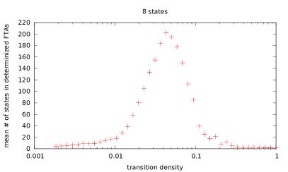
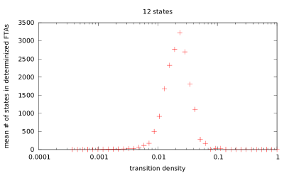
Figure 1: Graphs plotting the mean size of the determinized FTAs obtained by determinization over the density for FTAs of size $8$ and $12$. Minimization reduces the mean size, but does not move the peak.

Our experiments confirm the theoretical predictions. A peak in the mean size of the determinized FTAs can be observed where it is predicted. Exemplary graphs for setting (A) and $n\in\{8,12\}$ are presented in Figure 1 on a logarithmic scale. Since these graphs appear to be log-normal distributions, we computed the mean and the variance of these log-normal distributions, interpreting the density as the random variable and the number of states as the frequency. The relevant statistics are reported in Table 1 for setting (A). All predicted densities are in the confidence interval for the confidence level $p>.95$ (that is, the predicted density is within $1.96\cdot\sigma$ distance of the observed mean, where $\sigma$ is the standard deviation).

It is worth noting that the location of the peak does not change between settings (A) and (B). This means that the size of the alphabet of binary symbols does not influence the hardness of the problem; the only difference is the size of the resulting determinized FTAs, which is generally larger in setting (B). Also, minimization does not change the location of the peak, which means that hard instances for determinization are also hard instances for minimization. In addition, we also performed experiments that confirmed the similar result of [3] for finite-state string automata using the string automata toolkit FSM<2.0> of [7].

$d_{\_}2\,\backslash\,n$	2	4	6	7	8	9	10	11	12	13
.01				7%	11%	18%	27%	38%	50%	64%
.05			68%	82%	92%	98%	99%	100%	100%	100%
.10		54%	90%	96%	99%	99%	100%	100%	100%	100%
.25		83%	97%	98%	99%	100%	100%	100%	100%	100%
.50	47%	88%	96%	98%	100%	100%	100%	100%	100%	100%

Table 2: Ratio of trim FTAs in a set of randomly generated FTAs parameterized by density $d_{\_}2$ (rows) and number $n$ of states (columns). Blank entries indicate that no such experiment was performed.

References

- [1]
- [2] Walter S. Brainerd (1968): The Minimalization of Tree Automata. Inform. and Control 13(5), pp. 484–491, 10.1016/S0019-9958(68)90917-0.
- [3] Jean-Marc Champarnaud, Georges Hansel, Thomas Paranthoën & Djelloul Ziadi (2004): Random Generation Models for NFAs. J. Autom. Lang. Combin. 9(2/3), pp. 203–216.
- [4] John Doner (1970): Tree Acceptors and Some of Their Applications. J. Comput. System Sci. 4(5), pp. 406–451, 10.1016/S0022-0000(70)80041-1.
- [5] Ferenc Gécseg & Magnus Steinby (1984): Tree Automata. Akadémiai Kiadó, Budapest.
- [6] Ferenc Gécseg & Magnus Steinby (1997): Tree Languages. In Grzegorz Rozenberg & Arto Salomaa, editors: Beyond Words, chapter 1, Handbook of Formal Languages 3, Springer, pp. 1–68, 10.1007/978-3-642-59126-61.
- [7] Thomas Hanneforth (2010): fsm2 — A Scripting Language Interpreter for Manipulating Weighted Finite-State Automata. In: Proc. FSMNLP, LNCS 6062, Springer, pp. 13–30, 10.1007/978-3-642-14684-83.
- [8] Ondrej Lengál, Jirí Simácek & Tomás Vojnar (2012): VATA: A Library for Efficient Manipulation of Non-deterministic Tree Automata. In: Proc. TACAS, LNCS 7214, Springer, pp. 79–94, 10.1007/978-3-642-28756-57.
- [9] Ted Leslie (1995): Efficient Approaches to Subset Construction. Technical Report, University of Waterloo, Canada.
- [10] Jonathan May & Kevin Knight (2006): Tiburon: A Weighted Tree Automata Toolkit. In: Proc. CIAA, LNCS 4094, Springer, pp. 102–113, 10.1007/1181212811.
- [11] Slav Petrov, Leon Barrett, Romain Thibaux & Dan Klein (2006): Learning Accurate, Compact, and Interpretable Tree Annotation. In: Proc. COLING-ACL, Association for Computational Linguistics, pp. 433–440, 10.3115/1220175.1220230.
- [12] Sheng Yu (1997): Regular Languages. In Grzegorz Rozenberg & Arto Salomaa, editors: Word, Language, Grammar, chapter 2, Handbook of Formal Languages 1, Springer, pp. 41–110, 10.1007/978-3-642-59136-52.
- [13] Lynette van Zijl (1997): Generalized Nondeterminism and the Succinct Representation of Regular Languages. Ph.D. thesis, Stellenbosch University, South Africa.