Effects of Fluid Velocity Gradients on Heavy Quark Energy Loss

Abstract

We use holographic duality to analyze the drag force on, and consequent energy loss of, a heavy quark moving through a strongly coupled conformal fluid with non-vanishing gradients in its velocity and temperature. We derive the general expression for the drag force to first order in the fluid gradients. Using this general expression, we show that a quark that is instantaneously at rest, relative to the fluid, in a fluid whose velocity is changing with time feels a nonzero force. And, we show that for a quark that is moving ultra-relativistically, the first order gradient “corrections” become larger than the zeroth order drag force, suggesting that the gradient expansion may be unreliable in this regime. We illustrate the importance of the fluid gradients for heavy quark energy loss by considering a fluid with one-dimensional boost invariant Bjorken expansion as well as the strongly coupled plasma created by colliding sheets of energy.

1 Introduction and Summary

The analysis of how a heavy quark moving through the strongly coupled liquid quark-gluon plasma produced in ultrarelativistic heavy ion collisions loses energy and, subsequently, diffuses in the flowing plasma is of considerable theoretical interest because experimentalists are developing the detectors and techniques needed to use heavy quarks as ‘tracers’ or ‘probes’ of the strongly coupled liquid. If one assumes that the interactions between the heavy quark and the quark-gluon plasma are weak then perturbative techniques originally formulated for energetic light quarks Gyulassy:1993hr ; Baier:1996kr ; Baier:1996sk ; Zakharov:1997uu can be employed to analyze heavy quark energy loss Dokshitzer:2001zm .

The discovery that the plasma produced in heavy ion collisions is a strongly coupled liquid has prompted much interest in the real-time dynamics of strongly coupled non-Abelian plasmas and in the dynamics of heavy quarks therein. Although it remains to be seen to what degree treating all aspects of the dynamics of heavy quarks as strongly coupled is a good approximation, this approach is certainly of value as a benchmark: thorough understanding of the physics in this tractable setting can provide valuable qualitative insights. What makes these calculations tractable is holographic duality, which maps questions of interest onto calculations done via a dual gravitational description of the strongly coupled plasma and the heavy quark probe. The simplest theory in which these holographic calculations can be done is strongly coupled ${\cal N}=4$ supersymmetric Yang-Mills (SYM) theory in the large number of colors (large $N_{c}$) limit, whose plasma with temperature $T$ is dual to classical gravity in a 4+1-dimensional spacetime that contains a $3+1$-dimensional horizon with Hawking temperature $T$ and that is asymptotically anti–deSitter (AdS) spacetime, with the heavy quark represented by a string moving through this spacetime Maldacena:1997re ; Witten:1998qj ; Karch:2002sh ; Herzog:2006gh ; Gubser:2006bz ; CasalderreySolana:2006rq . The earliest work on heavy quark dynamics in the equilibrium plasma of strongly coupled ${\cal N}=4$ SYM theory Herzog:2006gh ; Gubser:2006bz ; CasalderreySolana:2006rq yielded determinations of the drag force felt by a heavy quark moving through the static plasma and the diffusion constant that governs the subsequent diffusion of the heavy quark once its initial motion relative to the static fluid has been lost due to drag. The basic picture of heavy quark dynamics that emerges, with all but the initially most energetic heavy quarks being rapidly slowed by drag and then becoming tracers diffusing within the (moving) fluid, is qualitatively consistent with early experimental investigations Adare:2006nq . For a review, see Ref. CasalderreySolana:2011us . Subsequently, the holographic calculational techniques were generalized to any static plasmas whose gravitational dual has a 4+1-dimensional metric that depends only on the holographic (i.e. ‘radial’) coordinate in Ref. Herzog:2006se and heavy quark energy loss and diffusion has by now been investigated in the equilibrium plasmas of many gauge theories with gravitational duals Caceres:2006dj ; Caceres:2006as ; Matsuo:2006ws ; Nakano:2006js ; Talavera:2006tj ; Gubser:2006qh ; Bertoldi:2007sf ; Liu:2008tz ; Gursoy:2009kk ; HoyosBadajoz:2009pv ; Bigazzi:2009bk ; NataAtmaja:2010hd ; Chernicoff:2012iq ; Fadafan:2012qu .

More recently, in Ref. Chesler:2013cqa we and a coauthor have calculated how the drag force and energy loss rate of a heavy quark moving through the far-from-equilibrium matter present just after a collision compares to that in strongly coupled plasma close to equilibrium. We studied the energy loss of a heavy quark moving through the debris produced by the collision of planar sheets of energy in strongly coupled SYM theory introduced in Ref. Chesler:2010bi and analyzed there and in Refs. Casalderrey-Solana:2013aba ; Chesler:2013lia . The matter produced in these collisions is initially far from equilibrium but then rapidly hydrodynamizes: its expansion and cooling is described well by viscous hydrodynamics after a time $t_{\rm hydro}$ that is at most around $(0.7-1)/T_{\rm hydro}$, where $T_{\rm hydro}$ is the effective temperature defined from the fourth root of the energy density at the hydrodynamization time $t_{\rm hydro}$. In Ref. Chesler:2013cqa we computed the drag force on a heavy quark moving through the initially far-from-equilibrium matter and the subsequent hydrodynamic fluid. We compared our results to what the drag force would have been in an equilibrium fluid with the same instantaneous energy density, and found that there is no dramatic “extra” energy loss in the far-from-equilibrium matter. However, even at late times when the expansion of the fluid is well-described by viscous hydrodynamics we found deviations between the actual drag force and what the drag force would have been in a spatially homogeneous equilibrium fluid with the same energy density. That is, we found that the gradients in the actual fluid do affect the drag force felt by the heavy quark moving through the fluid. Our goal in the present paper is a thorough investigation of the effects of gradients in the temperature and velocity of the fluid, up to first order, on the drag force.

We begin by computing the drag force on a heavy quark moving through a fluid whose own motion is only in one direction, which we shall take to be the $z$-direction. If we denote the fluid $4-$velocity by $u^{\mu}$ then at this stage the only gradients that we are considering are $\partial_{z}u^{z}$ and $\partial_{t}u^{z}$ as well as $\partial_{z}T$ and $\partial_{t}T$. Throughout this paper, we shall only work to first order in spatial gradients and time derivatives of the fluid temperature and velocity. The gravitational dual for a slowly changing fluid, including the effects of first order derivatives but neglecting higher derivatives, was first obtained in Ref. Bhattacharyya:2008jc , where Einstein’s equations in the 4+1-dimensional gravitational theory were solved to first order in gradients in the boundary coordinates and exactly in the radial direction. In Section 2.1 we describe this metric, for the case where the fluid motion is only in one direction, and then in Section 2.2 we introduce a heavy quark, described in the gravitational theory by a string. The endpoint lives at the boundary of the AdS space, where it follows the trajectory of the heavy quark of interest. We shall assume that it is being dragged at some constant velocity $\vec{\beta}$, which may or may not be parallel to the direction of motion of the fluid. In Section 2.2, with the gravitational metric describing the fluid in hand, we formulate and solve the string equations of motion, which is to say that we calculate the shape of the string attached to the heavy quark, including effects of fluid gradients up to first order. In Section 3.1 we use the string profile to calculate the flux of momentum down the string, which determines the drag force on the heavy quark. We first do the calculation in the fluid rest frame and then boost the result to any frame in Section 3.2. In Section 3.3 we generalize to the case in which the fluid has an arbitrary velocity and in which any of the gradients $\partial_{\alpha}u^{\beta}$ can be nonzero.

By analyzing the case in which the quark is moving with an ultrarelativistic velocity relative to the fluid we find indications that our results may not be valid in the limit in which the Lorentz factor $\gamma$ of the quark velocity is large, even if the quark mass $M\rightarrow\infty$ limit has been taken first and even if fluid gradients are small. We find that in the $\gamma\rightarrow\infty$ limit the “correction” to the drag force that is first order in fluid gradients is larger than the leading (i.e. zeroth order) term by a factor that is ${\cal O}(\gamma^{1/2})$. This suggests that the gradient expansion may not be valid in this regime. That is, even if higher order gradients are small enough that they are not important in describing the fluid motion itself their effects on the drag force may become important at large enough $\gamma$.

In Section 4, we consider three consequences of our general result for the first order effects of fluid gradients on the drag force exerted by the fluid on the heavy quark. First, we point out that even if the quark has no velocity relative to the fluid the drag force on it is nonzero as long as the time derivative of the fluid velocity is nonvanishing. Next, we consider two explicit examples of a fluid whose motion is only in one direction. First, we analyze the drag force on a heavy quark moving through a fluid that is undergoing boost-invariant expansion in the $z$-direction, à la Bjorken. We show that even though there are gradients in this fluid, a quark that is moving along with the fluid feels no drag force. A quark whose velocity includes a component perpendicular to the direction of motion of the fluid feels a drag force that is affected by the fluid gradients. And, last of all, we return to the colliding sheets of energy density that motivated our investigation, showing that our general expression for the effects of fluid gradients on the drag force to first order does a good job of explaining the explicit results obtained in Ref. Chesler:2013cqa , in many cases quantitatively and qualitatively in all cases, even those where the results of Ref. Chesler:2013cqa appear counter-intuitive. In Section 5 we look ahead to new directions whose investigation is motivated by our results.

2 Hydrodynamic fluid and a heavy quark moving through it

2.1 Gravitational description of a moving fluid

We begin with a brief description of the dual gravitational description of the stress-energy tensor for the conformal fluid of strongly coupled ${\cal N}=4$ SYM theory at nonzero temperature, undulating in some generic way according to the laws of hydrodynamics. We shall work only to first order in fluid gradients. In order to keep our expressions tractable on a first pass through the calculation, we shall then specialize to the case of a fluid that fills 3-dimensional space but that moves only along a single axis, flowing in some generic way along the $z$-direction. (Toward the end of Section 3 we shall lift this restriction, returning there to the case of generic hydrodynamic motion in 3+1 dimensions, still working only to first order in gradients which is to say still assuming that the spatial and temporal variation of the thermodynamic variables and the fluid velocity occur only on length and time scales that are much longer than $1/T$, with $T$ the fluid temperature.)

The stress-energy tensor for the conformal fluid of ${\cal N}=4$ SYM theory flowing hydrodynamically in $3+1$-dimensions with a temperature $T$ and $4$-velocity $u^{\mu}$ that vary as functions of space and time is given to first order in gradients by

$$\frac{8\pi^{2}}{N_{c}^{2}}T^{\mu\nu}=\frac{1}{b^{4}}\left(\eta^{\mu\nu}+4u^{\mu}u^{\nu}\right)-\frac{2}{b^{3}}\sigma^{\mu\nu},$$ (1)

where $b\equiv 1/(\pi T)$ is the inverse temperature, $\eta^{\mu\nu}=\text{diag}(-1,1,1,1)$ is the Minkowski metric, and

$$\sigma^{\mu\nu}=\frac{1}{2}P^{\mu\alpha}P^{\nu\beta}(\partial_{\alpha}u_{\beta}+\partial_{\beta}u_{\alpha})-\frac{1}{3}P^{\mu\nu}\partial_{\alpha}u^{\alpha}$$ (2)

is the symmetric tensor encoding the first order contributions of fluid gradients, with the projectors transverse to $u^{\mu}$ defined by $P^{\mu\nu}\equiv\eta^{\mu\nu}+u^{\mu}u^{\nu}$. With our metric conventions, $u^{\mu}$ is normalized such that $u^{\mu}u_{\mu}=-1$. The stress-energy tensor (1) describes a fluid whose equation of state is $P=\varepsilon/3$, where $P$ and $\varepsilon$ are its pressure and energy density respectively, and whose shear and bulk viscosities are given by $\eta=s/(4\pi)$ and $\zeta=0$, where $s$ is the entropy density of the fluid. $P=\varepsilon/3$ and $\zeta=0$ follow just from conformal invariance. $4\pi\eta/s=1$ for the fluid in any non-Abelian gauge theory with a dual gravitational description, in the strong coupling and large-$N_{c}$ limit Policastro:2001yc ; Kovtun:2003wp ; Buchel:2003tz ; Kovtun:2004de . Note that the stress-energy tensor depends on symmetric combinations of the fluid gradients $\partial_{\alpha}u_{\beta}$ and is independent of the fluid vorticity

$$\tilde{\omega}^{\mu}\equiv\frac{1}{2}\epsilon^{\mu\nu\alpha\beta}u_{\nu}\partial_{\alpha}u_{\beta}\,,$$ (3)

because the underlying microscopic theory does not violate time-reversal or parity symmetry. The vorticity will nevertheless play a role in our considerations later. Hydrodynamics is the statement that the fluid variables satisfy energy and momentum conservation,

$$\partial_{\mu}T^{\mu\nu}=0\ .$$ (4)

It is easy to see that, to first order in gradients, the hydrodynamic equations (4) determine the spatial and temporal variation of the temperature, or the inverse temperature $b$, uniquely in terms of the spatially and temporally varying fluid velocities:

$$\partial_{\mu}b=b\left(u^{\nu}\partial_{\nu}u_{\mu}-\frac{1}{3}u_{\mu}\partial_{\alpha}u^{\alpha}\right).$$ (5)

We shall use this relation below.

The dual gravitational description of the fluid with stress-energy tensor (1) was obtained in Ref. Bhattacharyya:2008jc . (These authors worked to second order in gradients. We shall quote their results only to first order.) Upon introducing a bookkeeping parameter $\epsilon$ that we shall use to count powers of gradients and that we shall in the end set to $\epsilon=1$, the $4+1$-dimensional metric in the dual gravitational description of the fluid takes the form

$$ds^{2}=\left(G_{MN}^{(0)}+\epsilon\,G_{MN}^{(1)}\right)dX^{M}dX^{N}$$ (6)

where $X^{M}\equiv(x^{\mu},r)$. The first term in (6) is given by

$$\begin{split}&G_{MN}^{(0)}dX^{M}dX^{N}=-2u_{\mu}dx^{\mu}dr-r^{2}f(br)u_{\mu}u_{\nu}dx^{\mu}dx^{\nu}+r^{2}P_{\mu\nu}dx^{\mu}dx^{\nu}\end{split}$$ (7)

where $f(x)\equiv 1-1/x^{4}$. If we set $u^{\mu}=(1,0,0,0)$ everywhere, the metric (7) describes a static AdS black brane with an event horizon at $r=1/b$ and with the AdS boundary located at $r=\infty$. This is the gravitational dual of the static ${\cal N}=4$ SYM plasma in equilibrium with a uniform and constant temperature $T=1/(\pi b)$. The coordinates $X^{M}$ that we are using to describe the spacetime, chosen in such a way that the metric has no $dr^{2}$ term and has no singularities at $r=1/b$, are referred to as in-falling Eddington-Finkelstein coordinates. With a generic choice of $u^{\mu}$, varying as a function of $x^{\mu}$, at any given $x^{\mu}$ the metric (7) is obtained by boosting the AdS black brane metric by the boost that takes you from the instantaneous fluid rest frame, where $u^{\mu}=(1,0,0,0)$, to the frame in which $u^{\mu}$ takes on the value of interest. The metric (7) is therefore often said to describe a boosted black brane, but it is important to remember that $b$ and $u^{\mu}$ are in fact varying. It describes a black brane whose horizon is undulating, as is its entire metric. Note that although $r=1/b$ is the horizon of the static black brane, once $1/b$ is undulating the global event horizon of the metric (6) need no longer be located at $r=1/b$. Gradient corrections to the position of the event horizon have been computed in Ref. Bhattacharyya:2008xc . The metric (7) is the zeroth approximation to the gravitational dual of the moving fluid; it would be a complete description if gradients made no contribution to the fluid stress-energy tensor, which is to say if the fluid were an ideal fluid with zero shear viscosity.

The second term in the metric (6) is the dual gravitational description of the contribution of first order gradients in $u^{\mu}$ and $b$ to the fluid stress-energy tensor. It is given by Bhattacharyya:2008jc

$$\begin{split}&G_{MN}^{(1)}dX^{M}dX^{N}=2r^{2}b\,F(br)\sigma_{\mu\nu}dx^{\mu}dx^{\nu}+\frac{2}{3}r\,u_{\mu}u_{\nu}\partial_{\lambda}u^{\lambda}dx^{\mu}dx^{\nu}-r\,u^{\lambda}\partial_{\lambda}(u_{\mu}u_{\nu})dx^{\mu}dx^{\nu}\end{split}$$ (8)

where

$$F(x)\equiv\frac{1}{4}\left[\log\left(\frac{(1+x)^{2}(1+x^{2})}{x^{4}}\right)-2\arctan x+\pi\right].$$ (9)

We are working in a gauge in which $G^{(1)}_{Mr}=0$. The metric (8) is a good approximation to the gravitational dual of the hydrodynamics of the flowing conformal fluid as long as the length scale $L$ over which $b$ and $u^{\mu}$ vary satisfies $L\gg b$.

In the next subsection, we will compute the profile of the string that hangs “down” into the bulk metric $G_{MN}$ from the heavy quark. To determine the profile of the string at the time $t$ at which the heavy quark is located at a particular position $\vec{x}$, it will prove convenient to do the calculation in the frame in which the fluid is at rest at $\vec{x}$ at the instant of time $t$, which is to say the frame in which $u^{\mu}(\vec{x},t)=(1,0,0,0)$. In making this choice we do not lose any generality since we can of course later boost the result of our calculation to any frame that we like. In order to do the calculation in the instantaneous fluid rest-frame it will be helpful to have the metric $G_{MN}$ in this frame, which we obtain by setting $u^{\mu}=(1,0,0,0)$ in (7) and (8), keeping derivatives of $u^{\mu}$. At the same time, since we will calculate the drag force on a heavy quark located at $x^{\mu}=0$ we expand $b(x^{\nu})$ and $u^{\mu}(x^{\nu})$ around $x^{\nu}=0$ in (7), keeping only terms that are first order in their gradients. Combining (7) and (8), the metric then takes the form

$$\begin{split}&G_{MN}dX^{M}dX^{N}=2dtdr-r^{2}f(br)dt^{2}+r^{2}dx_{i}dx_{i}\\ &+\epsilon\left(-2x^{\mu}\partial_{\mu}u_{i}drdx^{i}-2x^{\mu}\partial_{\mu}u_{i}r^{2}(1-f(br))dtdx^{i}-4\frac{x^{\mu}\partial_{\mu}b}{b^{5}r^{2}}dt^{2}\right.\\ &\left.+2br^{2}F(br)\sigma_{ij}dx^{i}dx^{j}+\frac{2}{3}r\partial_{i}u_{i}dt^{2}+2r\partial_{t}u_{i}dtdx^{i}\right)\ ,\end{split}$$ (10)

which is the form that we shall need.

We shall begin by doing the calculation for a fluid that is only moving in one direction, that we shall choose to be the $z$-direction. In this case, when we boost to the instantaneous rest-frame in which $u^{\mu}(\vec{x},t)=(1,0,0,0)$ the only non-vanishing gradients are

$$\partial_{t}b(t,z)\neq 0,\quad\partial_{z}b(t,z)\neq 0,\quad\partial_{t}u^{3}(t,z)\neq 0,\quad\partial_{z}u^{3}(t,z)\neq 0,$$ (11)

with

$$\partial_{\mu}u^{\perp}=\partial_{\perp}u^{\nu}=\partial_{\perp}b=0.$$ (12)

This fluid configuration will not be sufficient for us to determine the drag force in the most general configuration, in particular because in this configuration the fluid has zero vorticity. However, we shall see by the end of Section 3 that it suffices to get us most of the way. Upon making this simplifying assumption, conservation of the stress-energy tensor (5) takes on the particularly simple form

$$\begin{split}3\partial_{t}b(t,z)&=b(t,z)\partial_{z}u^{3}(t,z),\\ \partial_{z}b(t,z)&=b(t,z)\partial_{t}u^{3}(t,z).\end{split}$$ (13)

We will return to the consideration of a general fluid configuration only in Section 3.3.

2.2 Gravitational description of a moving heavy quark

The dual gravitational string of a quark with mass $M$ at the spacetime point $x^{\mu}=0$ and moving with velocity $\vec{\beta}$ is, in the $M\rightarrow\infty$ limit, a string whose endpoint is at $x^{\mu}=0$ moving with velocity $\vec{\beta}$ along the AdS boundary, namely at $r\rightarrow\infty$. The dynamics of the string is described by the Nambu-Goto action

$$S_{\rm NG}=-\frac{\sqrt{\lambda}}{2\pi}\int d\tau d\sigma\sqrt{-g(\tau,\sigma)}$$ (14)

where the string tension is $\frac{\sqrt{\lambda}}{2\pi}$, where $\lambda=g^{2}N_{c}$ is the ’t Hooft coupling, and where $g(\tau,\sigma)=\det g_{ab}(\tau,\sigma)$ with $g_{ab}(\tau,\sigma)$ the induced metric on the world-sheet, namely

$$\begin{split}g_{ab}(\tau,\sigma)&=G_{MN}\partial_{a}X^{M}(\tau,\sigma)\partial_{b}X^{N}(\tau,\sigma).\end{split}$$ (15)

We shall parametrize the string world-sheet in such a way that

$$\begin{split}t(\tau,\sigma)&=\tau,\\ r(\tau,\sigma)&=\sigma.\end{split}$$ (16)

We shall assume that the string is being dragged along with a constant velocity $\vec{\beta}$. Because we are treating the case where the fluid motion is only in the $z$-direction, without loss of generality we can choose $\vec{\beta}=(\beta_{x},0,\beta_{z})$. We can think of the motion of the quark as being due to a force exerted on it by some electric field, with respect to which the quark is charged. Our task is to determine the force required to drag the quark, working to leading order in the fluid gradients. The first step in the calculation, which we shall carry out in this section, is the determination of the string profile, again to leading order in fluid gradients.

We denote the string profile to first order in gradients by

$$\vec{x}(\tau,\sigma)=\vec{x}_{0}(\tau,\sigma)+\epsilon\,\vec{x}_{1}(\tau,\sigma)$$ (17)

where $\vec{x}_{0}(\tau,\sigma)$ is the string profile in the case of an equilibrium fluid with a constant temperature that is moving with some uniform velocity, which is to say in the absence of any gradients in the fluid velocity or $b$. In the instantaneous fluid rest-frame in which we are working this means that $u^{\mu}=(1,0,0,0)$ and all gradients vanish. This “trailing string” solution was first obtained in Refs. Herzog:2006gh ; Gubser:2006bz and is given by

$$\vec{x}_{0}(\tau,\sigma)=\vec{\beta}\left(\tau-b\left(\tan^{-1}(b\sigma)-\frac{\pi}{2}\right)\right)\ ,$$ (18)

where we note that at $\sigma\rightarrow\infty$ the endpoint of the string follows the trajectory of the heavy quark. We will need to differentiate $\vec{x}_{0}$, and to that end we need to keep track of how it depends on $u^{\mu}$, namely

$$\vec{x}_{0}(\tau,\sigma)=\vec{\beta}\tau-b\left(u^{0}\vec{\beta}-\vec{u}\right)\left(\tan^{-1}(b\sigma)-\frac{\pi}{2}\right)\ .$$ (19)

The function $x_{1}(\tau,\sigma)$ in (17) encodes the corrections to the zeroth order profile $\vec{x}_{0}(\tau,\sigma)$ due to fluid gradients, up to first order in those gradients. It must vanish in the $\sigma\rightarrow\infty$ limit. Our task in the remainder of this section is to calculate $x_{1}(\tau,\sigma)$.

The equations of motion for the string are obtained by extremizing the Nambu-Goto action with respect to the function $\vec{x}(\tau,\sigma)$. To zeroth order we obtain $\vec{x}_{0}(\tau,\sigma)$. The function $\vec{x}_{1}(\tau,\sigma)$ is determined from

$$\partial_{\tau}\left(\frac{\delta\mathcal{L}}{\delta(\partial_{\tau}\vec{x}_{1})}\right)+\partial_{\sigma}\left(\frac{\delta\mathcal{L}}{\delta(\partial_{\sigma}\vec{x}_{1})}\right)=\frac{\delta\mathcal{L}}{\delta\vec{x}_{1}}\ .$$ (20)

Since the terms that are linear in gradients in (10) arose either directly from (8) or via expanding (7) to first order about $x^{\mu}=0$, the terms in (20) that are first order in gradients can depend on time at most linearly, meaning that $x_{1}(\tau,\sigma)$ takes the form

$$\vec{x}_{1}(\tau,\sigma)=b\,\tau\,\vec{h}(\sigma)+b\,\vec{g}(\sigma)\ ,$$ (21)

with $\vec{h}(\sigma)$ and $\vec{g}(\sigma)$ being dimensionless functions that we must determine, that both have only $x$- and $z$-components, and that both vanish at $\sigma\rightarrow\infty$.

The terms in the Euler-Lagrange equation (20) that are proportional to $\tau$ depend only on $\vec{h}(\sigma)$, not on $\vec{g}(\sigma)$. It is in fact possible to guess the form of $\vec{h}(\tau)$. However, determining it by explicit solution is instructive, so we shall follow that route. Integrating the Euler-Lagrange equations for $\vec{h}(\sigma)$ once yields

$$\begin{split}h_{x}^{\prime}(\sigma)&=\frac{c_{hx}\gamma^{2}(b^{2}\sigma^{2}+1)^{2}-2\beta_{x}D_{t}b(\gamma^{2}+2b^{2}\sigma^{2}+1)}{(\gamma^{2}-b^{2}\sigma^{2})(b^{2}\sigma^{2}+1)^{2}},\\ h_{z}^{\prime}(\sigma)&=\frac{1}{\left(b^{4}\sigma^{4}-\gamma^{2}\right)}\times\\ &\left(\frac{b\left(b^{4}\sigma^{4}+2b^{2}\sigma^{2}-\gamma^{2}+2\right)D_{t}u^{3}}{\left(b^{2}\sigma^{2}+1\right)}+\frac{2\beta_{z}\left(2b^{2}\sigma^{2}+\gamma^{2}+1\right)D_{t}b}{\left(b^{2}\sigma^{2}+1\right)^{2}}-\gamma^{2}c_{hz}\right),\end{split}$$ (22)

where by ^′ we mean $d/d\sigma$ and where

$$D_{t}\equiv\partial_{t}+\beta^{i}\partial_{i}=\partial_{t}+\beta_{z}\partial_{z}$$ (23)

is the convective derivative along the path of the quark, with the second equality valid here because the only nonzero gradients are in the $z$-direction, where $\gamma=(1-\vec{\beta}^{2})^{-1/2}$ is the Lorentz factor for the heavy quark, and where $c_{hx}$ and $c_{hz}$ are integration constants that we must now fix. The expressions for $\vec{h}^{\prime}(\sigma)$ have a first order pole at the radial position

$$\sigma=\frac{\sqrt{\gamma}}{b}\ ,$$ (24)

which in the case of the static fluid is identified as the location of the worldsheet horizon $\sigma_{\rm ws}\equiv\sqrt{\gamma}/b$ that arises in the calculation of $\vec{x}_{0}(\tau,\sigma)$ in a static fluid Herzog:2006gh ; Gubser:2006bz .

We have found that the position on the worldsheet where the integration constants are fixed, $\sigma=\sqrt{\gamma}/b$, is the same as it would be in a static homogeneous fluid with the same instantaneous temperature. This means that our results disagree with those of Refs. Abbasi:2012qz ; Abbasi:2013mwa : those authors assumed that the influence of fluid gradients on the drag force could be described via a dependence of this radial position on the fluid gradients. We now see by explicit calculation that, at least to first order, there is no such dependence. And, indeed our results for the drag force that we shall present in Section 3 do differ from those in Refs. Abbasi:2012qz ; Abbasi:2013mwa .

As in the static fluid calculation of Refs. Herzog:2006gh ; Gubser:2006bz , in order to obtain a regular string profile across the world-sheet horizon we must choose the integration constants in (22) in such a way that the numerators on the right-hand sides of (22) vanish at the same $\sigma$ at which the denominators vanish, i.e. at the world-sheet horizon. This requirement uniquely determines the integration constants to be

$$\begin{split}c_{hx}&=\frac{2\beta_{x}D_{t}b}{\gamma^{2}},\quad c_{hz}=2\frac{bD_{t}u^{3}+\beta_{z}D_{t}b}{\gamma^{2}}.\end{split}$$ (25)

The expressions (22) can then be integrated again, with the new integration constants being fixed via the requirement that $\vec{h}(\sigma)$ vanishes at $\sigma\rightarrow\infty$. Doing so yields

$$\begin{split}h_{x}(\sigma)=&\frac{\beta_{x}}{b}\left(\frac{\pi}{2}-\tan^{-1}(b\sigma)-\frac{b\sigma}{b^{2}\sigma^{2}+1}\right)D_{t}b,\\ h_{z}(\sigma)=&\frac{\beta_{z}}{b}\left(\frac{\pi}{2}-\tan^{-1}(b\sigma)-\frac{b\sigma}{b^{2}\sigma^{2}+1}\right)D_{t}b-\left(\frac{\pi}{2}-\tan^{-1}(b\sigma)\right)D_{t}u^{3}\ ,\end{split}$$ (26)

which we can denote more simply by

$$b\,\vec{h}(\sigma)=D_{t}\vec{x}_{0}(\tau,\sigma)\Big{|}_{\tau=0}\,,$$ (27)

a result that we now see could have been guessed. So, we have shown that

$$\vec{x}(\tau,\sigma)=\vec{x}_{0}(\tau,\sigma)+\epsilon\,\tau D_{t}\vec{x}_{0}(\tau,\sigma)\Bigl{|}_{\tau=0}+\epsilon\,b\,\vec{g}(\sigma)$$ (28)

to the order at which we are working, and our task now is to find $\vec{g}(\sigma)$.

Upon using the solution for $\vec{h}(\sigma)$, the Euler-Lagrange equations become differential equations for $\vec{g}(\sigma)$. As in the determination of $\vec{h}(\sigma)$, we integrate the differential equations for $\vec{g}(\sigma)$ once, obtaining expressions for $\vec{g}^{\prime}(\sigma)$. Again as before, these expressions have poles at $\sigma=\sigma_{\rm ws}$ and the requirement that the string profile must be regular there can be used to fix the integration constants in the expressions for $\vec{g}^{\prime}(\sigma)$. Upon so doing, we find

$$\begin{split}&g_{x}^{\prime}(\sigma)=\frac{b^{2}\beta_{x}\beta_{z}\left(\left(-\pi/2+\tan^{-1}(b\sigma)\right)\left(b^{2}\sigma^{2}+3\right)+b\sigma\right)}{\left(b^{2}\sigma^{2}+1\right)^{2}}\partial_{t}u^{3}+\frac{b^{2}\beta_{x}}{3}\partial_{z}u^{3}\times\\ &\left(\left(\gamma^{2}\left(3\beta_{z}^{2}+1\right)+1\right)\frac{c_{1}\left(-b^{2}\sigma^{2}\right)-c_{1}(-\gamma)}{\gamma^{2}-b^{4}\sigma^{4}}-\frac{1}{(\sqrt{\gamma}+b\sigma)(\gamma+b^{2}\sigma^{2})}-\frac{\frac{\pi}{2}-\tan^{-1}(b\sigma)}{1+b^{2}\sigma^{2}}\right),\\ &g_{z}^{\prime}(\sigma)=b^{2}\left(\frac{b^{2}\sigma^{2}\left(\beta_{z}^{2}-1\right)+3\beta_{z}^{2}-1}{\left(b^{2}\sigma^{2}+1\right)^{2}}\tan^{-1}(b\sigma)\right.\\ &\left.-\frac{1}{2}\left(\frac{\sqrt{\gamma}-b\sigma}{\gamma(b^{2}\sigma^{2}+\gamma)}+\frac{2\beta_{z}^{2}(\pi-b\sigma)}{\left(b^{2}\sigma^{2}+1\right)^{2}}-\frac{\pi(1-\beta_{z}^{2})}{b^{2}\sigma^{2}+1}+\frac{1}{\gamma(b\sigma+\sqrt{\gamma})}\right)\right)\partial_{t}u^{3}\\ &+\frac{b^{2}\beta_{z}\left(5\left(b\sigma+\sqrt{\gamma}\right)\left(b^{2}\sigma^{2}+\gamma\right)\left(\frac{\pi}{2}-\tan^{-1}(b\sigma)\right)-\left(b^{2}\sigma^{2}+1\right)\right)}{3\left(b^{2}\sigma^{2}+1\right)\left(b\sigma+\sqrt{\gamma}\right)\left(b^{2}\sigma^{2}+\gamma\right)}\partial_{z}u^{3},\end{split}$$ (29)

where we have defined the function

$$\begin{split}c_{1}(x)&\equiv\pi/2-\tan^{-1}(\sqrt{-x})-F(\sqrt{-x})\\ &=\frac{1}{4}\left(2\tan^{-1}\left(\frac{1}{\sqrt{-x}}\right)-\log\left(\frac{(1-x)(1+\sqrt{-x})^{2}}{x^{2}}\right)\right).\end{split}$$ (30)

(The way we have chosen the signs in this definition will prove convenient later.) We can see explicitly in (29) that $\vec{g}(\tau,\sigma)$ is regular at $\sigma=\sigma_{\rm ws}$. It is then possible to integrate the expressions (29) analytically, fixing the integration constants by the requirement that $\vec{g}(\tau,\sigma)=0$ at $\sigma\rightarrow\infty$. The resulting expressions for $g_{x}(\sigma)$ and $g_{z}(\sigma)$ are unwieldy and we shall not quote them here. In Section 4 we shall, however, plot the string profile for several choices of fluid flow and $\vec{\beta}$. In addition to being unwieldy, the expressions for $g_{x}(\sigma)$ and $g_{z}(\sigma)$ are not of direct utility because, as we shall see in Section 3, it is only $\vec{g}^{\prime}(\sigma)$ that enters into the calculation of the canonical momentum fluxes along the string and hence of the drag force.

3 Computing the drag force on the heavy quark

In this Section we calculate the drag force acting on the heavy quark moving through the strongly coupled fluid. If the fluid were static, as in the original calculations Herzog:2006gh ; Gubser:2006bz , the drag force would be a function of the temperature and the velocity $\vec{\beta}$ of the heavy quark. In the case that we are analyzing, where the fluid is moving but we work in the instantaneous fluid rest-frame, the drag force again depends on $b$ and $\vec{\beta}$ but, we shall show, it also depends upon the spatial gradients and time derivatives of $b$ and the fluid $4$-velocity $u^{\mu}$. After computing the drag force in the instantaneous fluid rest frame in Section 3.1 for the case in which the fluid motion is only along the $z$-direction, in Section 3.2 we boost the result to a frame in which the fluid at the location of the heavy quark has some nonzero velocity in the $z$-direction, $u^{3}\neq 0$. Then, in Section 3.3 we generalize our result to the case in which the motion of the fluid is not restricted to the $z$-direction and, in particular, may feature nonzero vorticity.

When the heavy quark is dragged through the fluid, in the dual gravitational description momentum and energy flow “down” the string that “hangs down” from the heavy quark at $r=\infty$, trailing into the bulk metric. In order to conserve energy and momentum, an external force must be exerted upon the heavy quark to keep it moving at constant velocity and (in the dual picture) to replace the energy and momentum flowing down the string. Consequently,

$$\partial_{\nu}T^{\nu\mu}=-f^{\mu}(\tau)\delta^{3}(\vec{x}-\vec{\beta}\tau)$$ (31)

where $f^{\mu}(\tau)$ is the drag force acting on the heavy quark, i.e., on the endpoint of the string at the $r=\infty$ boundary. The drag force at the boundary is given by Herzog:2006gh ; Gubser:2006bz

$$f^{\mu}(\tau)=\lim_{\sigma\to\infty}n_{M}\int d^{3}x\sqrt{-g}\mathcal{T}^{M\mu}$$ (32)

where $\mathcal{T}^{MN}$ is the stress-energy tensor of the string obtained by varying the Nambu-Goto action (14) with respect to the $G_{MN}$, and $n_{M}$ is the unit-vector normal to the boundary at $r\to\infty$. Because we are using the simple parametrization (16) of the world-sheet, the normal is simply $n_{M}=-\delta_{M5}$ and the relevant component of the string stress-energy tensor is

$$\mathcal{T}^{5\mu}(\tau,\vec{x},\vec{y},\sigma)=\eta^{\mu\nu}\frac{1}{\sqrt{-g}}\pi^{\sigma}_{\nu}(\tau,\sigma)\delta^{3}(\vec{y}-\vec{x})\,,$$ (33)

where the canonical energy/momentum fluxes along the string are obtained by varying $S_{\rm NG}$ with respect to $\partial_{\sigma}X^{\mu}$:

$$\pi^{\sigma}_{\mu}\equiv\frac{\delta S_{\rm NG}}{\delta(\partial_{\sigma}X^{\mu})}=-\frac{\sqrt{\lambda}}{2\pi}G_{\mu N}\frac{1}{\sqrt{-g}}\left[g_{\tau\sigma}\partial_{\tau}X^{N}-g_{\tau\tau}\partial_{\sigma}X^{N}\right].$$ (34)

Combining (32) and (33), the force acting on the quark at the boundary is given by

$$f^{\mu}(\tau)=-\frac{dp^{\mu}}{dt}(\tau)=-\lim_{\sigma\to\infty}\eta^{\mu\nu}\pi^{\sigma}_{\nu}(\tau,\sigma),$$ (35)

evaluated at the location of the heavy quark, $\vec{x}=\vec{\beta}\tau$. Because we have used the world-sheet parameterization (16) we have obtained the same expression obtained in Refs. Herzog:2006gh ; Gubser:2006bz ; the calculation of Ref. Chesler:2013cqa was done with a different world-sheet parametrization, one for which (32) yields an expression that differs from (35). Note also that we are using a sign convention opposite to that in Ref. Chesler:2013cqa . In the present paper, $f^{\mu}$ is the force exerted on the heavy quark by some external agency (eg. an electric field) in order to keep the quark moving with constant velocity. In the classic case of a quark moving with $\beta_{z}>0$ through a static plasma, $f^{z}>0$ and $dp^{z}/dt<0$. Note that $dp^{\mu}/dt$ refers to the energy/momentum lost by the quark (lost by the quark and gained by the plasma; in the dual description, lost by the quark and flowing down the string).

As is the case for any force, $f^{\mu}(\tau)$ is not a Lorentz $4$-vector. This is most easily seen via the expression $f^{\mu}=-dp^{\mu}/dt$, in which $p^{\mu}$ is a $4$-vector but $t$ is not boost-invariant. We see immediately that we can define a so-called proper force $F^{\mu}(\tau)$ that is a $4$-vector via

$$F^{\mu}(\tau)\equiv f^{\mu}(\tau)\frac{dt}{d\tau_{p}}=-\frac{dp^{\mu}}{d\tau_{p}}$$ (36)

where $\tau_{p}$ is the (boost-invariant) proper time of the quark. Because the heavy quark is moving with a constant velocity, $dt=\gamma d\tau_{p}$, with $\gamma\equiv 1/\sqrt{1-|\vec{\beta}|^{2}}$ the Lorentz factor for the heavy quark. Then the actual drag force $f^{\mu}$ and the proper drag force $F^{\mu}$ are simply related by

$$f^{\mu}(\tau)=\frac{1}{\gamma}F^{\mu}(\tau).$$ (37)

The distinction between actual and proper forces will play an important role in Sections 3.2 and 3.3.

Just as we did in the calculation of the string profile, we expand the drag force in powers of the fluid gradients, writing it as

$$f^{\mu}(\tau)=f_{(0)}^{\mu}(\tau)+\epsilon f_{(1)}^{\mu}(\tau),$$ (38)

where the first component $f_{(0)}^{\mu}(\tau)$ is the drag force when fluid gradients are neglected, first obtained in Refs. Herzog:2006gh ; Gubser:2006bz , and the second component $f_{(1)}^{\mu}(\tau)$ is proportional to fluid gradients and is the term that we will calculate in the remainder of this Section. In the instantaneous fluid rest frame, in which $u^{\mu}=(1,0,0,0)$, the spatial components of the force are given by Herzog:2006gh ; Gubser:2006bz

$$\vec{f}_{(0),\rm RF}(\tau)=\frac{\sqrt{\lambda}}{2\pi}\frac{\gamma}{b^{2}}\vec{\beta}$$ (39)

which shows that this contribution to the force is proportional to $\gamma\vec{\beta}$, which is to say proportional to $\vec{p}/M$. It is because the force is proportional to the momentum that it is referred to as a drag force. We can then boost this result to any other frame, in which the fluid at the location of the heavy quark has an instantaneous three-velocity $\vec{v}$ and a Lorentz factor $\gamma_{v}\equiv 1/\sqrt{1-|\vec{v}|^{2}}$ and, hence,

$$u^{\mu}=\gamma_{v}(1,\vec{v})\ .$$ (40)

It is also convenient to define the $4-$velocity of the heavy quark

$$w^{\mu}=\gamma(1,\vec{\beta})\ .$$ (41)

Upon boosting (39) to a frame in which $\vec{v}\neq 0$, the zeroth contribution to the drag force (i.e. the drag force obtained upon neglecting the effects of gradients) takes the form

$$f_{(0)}^{\mu}(\tau)=-\frac{\sqrt{\lambda}}{2\pi}\frac{1}{\gamma b^{2}}\left(s\,w^{\mu}+u^{\mu}\right),$$ (42)

where the scalar factor $s$ is defined by

$$s\equiv u^{\nu}w_{\nu}\ .$$ (43)

If the only nonzero component of $\vec{v}$ is $v_{z}$, we find $s=-\gamma\gamma_{v}(1-v_{z}\beta_{z})$. We shall calculate $f^{\mu}_{(1)}$ in the instantaneous fluid rest frame in Section 3.1, and in a more general frame in Section 3.2.

Before turning to our calculation, one further general remark will prove useful. Starting from (35) and (34), it is possible to show by explicit calculation that $w_{\mu}f^{\mu}(\tau)=0$. Written explicitly, this takes the form

$$\frac{dE}{dt}=\vec{\beta}\frac{d\vec{p}}{dt},$$ (44)

relating the rate of energy loss to the rate of momentum loss. Since $\vec{\beta}=\vec{p}/E$ this implies that $E^{2}=\vec{p}^{2}+M^{2}$ for some constant $M$, which is to say that if the quark starts out on-shell it stays on-shell.

3.1 Drag force in the instantaneous fluid rest frame

We now calculate the canonical momentum flux along the string to first order in gradients, $\pi^{\sigma}_{\mu,(1)}(\tau,\sigma)$, and use it to obtain the corresponding drag force $f_{(1)}^{\mu}(\tau)$ exerted on the heavy quark at the boundary. We calculate the drag force in the instantaneous fluid rest frame using the string profile given in Eqs. (26) and (29). We need to evaluate (34) to linear order in $\epsilon$ after expanding the metric $G_{\mu N}$, the induced metric $g_{ab}$, and derivatives of the string profile $\partial_{a}X^{N}$ in powers of $\epsilon$. Just as for the decomposition of the string profile in Eq. (28), we find that

$$\pi^{\sigma}_{\mu}(\tau,\sigma) =\pi^{\sigma}_{\mu,(0)}(\tau)+\epsilon\left(\tau\,D_{t}\pi^{\sigma}_{\mu,(0)}(\tau)\Big{|}_{\tau=0}+\pi^{\sigma}_{\mu,(1)}(\sigma)\right).$$ (45)

The leading term is independent of the radial coordinate $\sigma$ and, in the instantaneous fluid rest-frame, is given by

$$\pi^{\sigma}_{\mu,(0)}(\tau)=-\frac{\sqrt{\lambda}}{2\pi}\frac{1}{\gamma b^{2}}\left(\gamma w_{\mu}+\delta^{0}_{\mu}\right),$$ (46)

from which we obtain the result for the drag force absent any effects of the fluid gradients that we already quoted in Eq. (42). The term proportional to time $\tau$ in (45) is given by

$$\begin{split}&D_{t}\pi^{\sigma}_{\mu,(0)}(\tau)\Big{|}_{\tau=0}=\frac{\sqrt{\lambda}}{2\pi}\frac{1}{\gamma b^{2}}\times\left[\frac{2}{b}(\gamma w^{\mu}-\delta^{\mu}_{0})D_{t}b+(w^{\mu}w^{z}+\delta^{\mu}_{3})D_{t}u^{z}\right],\end{split}$$ (47)

where $D_{t}$ was defined in (23). We can neglect this term since it appears in (45) multiplied by $\tau$ and we are evaluating the drag force on the heavy quark at $\tau=0$.

The nontrivial part of the computation is the determination of $\pi^{\sigma}_{(1)}(\sigma)$. After collecting terms proportional to $\epsilon$ at $\tau=0$, we find that

$$\begin{split}\pi^{\sigma}_{x,(1)}(\sigma)&=\frac{\sqrt{\lambda}}{2\pi b}\gamma\beta_{x}\left[\beta_{z}\left(\frac{b\sigma}{b^{2}\sigma^{2}+1}+\pi-2\tan^{-1}(b\sigma)-\sqrt{\gamma}\right)\partial_{t}u^{3}+\right.\\ &\left.\frac{\left(\frac{b\sigma}{b^{2}\sigma^{2}+1}-\sqrt{\gamma}+\left(1+3\beta_{z}^{2}\right)\left(\frac{\pi}{2}-\tan^{-1}(b\sigma)\right)-c_{1}\left(-\gamma\right)\left(\gamma^{2}\left(1-3\beta_{z}^{2}\right)+1\right)\right)}{3}\partial_{z}u^{3}\right],\\ \pi^{\sigma}_{z,(1)}(\sigma)&=\frac{\sqrt{\lambda}}{2\pi b}\gamma\left[\left(-\frac{\beta_{x}^{2}b\sigma}{b^{2}\sigma^{2}+1}+\left(2\beta_{z}^{2}+1\right)\left(\frac{\pi}{2}-\tan^{-1}(b\sigma)\right)-\sqrt{\gamma}\left(1-\beta_{x}^{2}\right)\right)\partial_{t}u^{3}+\right.\\ &\left.\frac{\beta_{z}\left(\frac{b\sigma}{b^{2}\sigma^{2}+1}+(1-3\beta_{x}^{2})\left(\frac{\pi}{2}-\tan^{-1}(b\sigma)\right)-\sqrt{\gamma}-c_{1}\left(-\gamma\right)\left(\gamma^{2}\left(1-3\beta_{z}^{2}\right)-5\right)\right)}{3}\partial_{z}u^{3}\right],\end{split}$$ (48)

where $c_{1}(-\gamma)$ was defined in (30) and the conservation of the stress-energy tensor (13) has been used to eliminate $\partial_{t}b$ and $\partial_{z}b$ in favor of $\partial_{t}u^{3}$ and $\partial_{z}u^{3}$. We now determine the contributions of these canonical momentum fluxes to the drag force on the heavy quark at the boundary, which is to say we take the $\sigma\to\infty$ limit. The terms $\frac{b\sigma}{b^{2}\sigma^{2}+1}$ and $\frac{\pi}{2}-\tan^{-1}(b\sigma)$ vanish in this limit, and the contribution to the drag force that is first order in gradients is given by

$$\begin{split}f^{x}_{(1)}&=\frac{\sqrt{\lambda}}{2\pi b}\gamma\beta_{x}\left(\sqrt{\gamma}\beta_{z}\partial_{t}u^{3}+\frac{\sqrt{\gamma}+c_{1}\left(-\gamma\right)\left(\gamma^{2}\left(1-3\beta_{z}^{2}\right)+1\right)}{3}\partial_{z}u^{3}\right),\\ f^{z}_{(1)}&=\frac{\sqrt{\lambda}}{2\pi b}\gamma\left(\sqrt{\gamma}(1-\beta_{x}^{2})\partial_{t}u^{3}+\frac{\sqrt{\gamma}+c_{1}\left(-\gamma\right)\left(\gamma^{2}\left(1-3\beta_{z}^{2}\right)-5\right)}{3}\beta_{z}\partial_{z}u^{3}\right),\end{split}$$ (49)

with the $t$ component of the force given by $f^{t}_{(1)}=\beta_{x}f^{x}_{(1)}+\beta_{z}f^{z}_{(1)}$, ensuring that the quark stays on shell. The complete expression for the drag force is obtained by combining the contributions from (46) and (49).

Before turning to generalizations of this result, we end this subsection by remarking that both the terms proportional to $\partial_{t}u^{3}$ and the terms proportional to $\partial_{z}u^{3}$ in (49) are proportional to $\gamma^{3/2}$ for large $\gamma$. This is apparent for the terms proportional to $\partial_{t}u^{3}$. To see this for the terms proportional to $\partial_{z}u^{3}$, note that in the large-$\gamma$ limit

$$c_{1}(-\gamma)=-\frac{1}{3\gamma^{3/2}}+\mathcal{O}\left(\frac{1}{\gamma^{2}}\right)\ .$$ (50)

This means that for large enough $\gamma$, the contributions to the drag force that are first order in fluid gradients, namely (49), dominate over the zeroth order expression (39) for the drag force in the absence of fluid gradients. Comparing (39) and (49) we see that the first order contributions to the drag force are smaller than the zeroth order contributions when

$$\sqrt{\gamma}<\frac{1}{b\,\left|\partial_{t}u^{3}\right|}\quad{\rm and}\quad\sqrt{\gamma}<\frac{9}{5}\frac{1}{b\,\left|\partial_{z}u^{3}\right|}$$ (51)

or, using (13), when

$$\sqrt{\gamma}<\frac{1}{\left|\partial_{z}b\right|}\quad{\rm and}\quad\sqrt{\gamma}<\frac{3}{5}\frac{1}{\left|\partial_{t}b\right|}\ ,$$ (52)

with $\gamma$ and the gradients on the right-hand sides of all these expressions evaluated in the frame of reference in which the fluid is instantaneously at rest at the location of the moving heavy quark. This result suggests that at larger values of $\gamma$ the expansion of the drag force in powers of the fluid gradients may break down, although to be sure of this it would be useful to extend our calculation to higher order in gradients. At a qualitative level, what seems to be happening is that at large enough $\gamma$ the heavy quark sees a gradient in the fluid as sudden, and the gradient expansion of the drag force ceases to be valid. Note that the criterion for the validity of the hydrodynamic description of the fluid itself is $|\partial_{z}b|\ll 1$ and $|\partial_{t}b|\ll 1$, meaning that as long as the motion of the fluid is described well by hydrodynamics the limitation (52) on the values of $\gamma$ at which the gradient expansion can be used to describe the drag force on the heavy quark sets in at some $\gamma\gg 1$. As hydrodynamics itself breaks down, the range of validity of the gradient expansion in the calculation of the heavy quark drag force becomes smaller and smaller.

Note that for quarks with finite $M$ the description of the drag force in terms of a single trailing string is only valid for Liu:2006he ; CasalderreySolana:2007qw ; CasalderreySolana:2011us

$$\sqrt{\gamma}\ll\frac{M}{T\sqrt{\lambda}}\ ,$$ (53)

since the external force required to move a quark with mass $M$ at a larger $\gamma$ would result in copious pair-production of quark-antiquark pairs. However, we are working in the $M\rightarrow\infty$ limit throughout this paper, meaning that the criterion (53) by itself would allow us to consider arbitrarily large $\gamma$. Instead, even in the $M\rightarrow\infty$ limit the magnitude of the fluid gradients imposes new, lower, limits (52) on how large $\gamma$ can be, at least if one wishes to use a gradient expansion to calculate the drag force. These considerations motivate future extensions of our calculations, both to higher order in fluid gradients and to finite quark mass $M$. An analysis in which one takes the $\gamma\rightarrow\infty$ limit first, with finite mass quarks, and only later takes $M\rightarrow\infty$ would necessarily look very different from the analysis in this paper.

3.2 Generalizing to a frame in which the fluid is moving

In Section 3.1 we have calculated the drag force exerted on a heavy quark moving through the fluid, in the instantaneous fluid rest frame and in a fluid that is moving only along the $z$-direction, obtaining the result (49). We can now boost this result to a frame in which the fluid at the location of the heavy quark has velocity $\vec{v}=(0,0,v_{z})$, instead of being at rest. We do this by first constructing the proper force $F^{\mu}$ from $f^{\mu}$, according to (37), then applying a Lorentz transformation to the $4-$vector $F^{\mu}$, bringing it to the desired frame, then working out the value of $\gamma$ in the desired frame, and finally using (37) again to obtain $f^{\mu}$ in the new frame. The calculation, which is tedious but straightforward, yields the following expression for the drag force exerted on a heavy quark moving with velocity $\vec{\beta}$ through a fluid that is moving only along the $z$-direction and that has velocity $\vec{v}=(0,0,v_{z})$ at the location of the heavy quark:

$$\begin{split}f^{x}_{(1)}&=-\frac{\sqrt{\lambda}}{2\pi}\frac{s\gamma_{v}^{2}\beta_{x}}{3b}\Bigl{[}\partial_{t}v_{z}\left[c_{1}(s)\left(s^{2}+1\right)\gamma_{v}v_{z}+3c_{1}(s)s(s\gamma_{v}+\gamma)\Delta\beta_{z}+\sqrt{-s}\gamma_{v}(3\Delta\beta_{z}+v_{z})\right]\Bigr{.}\\ &\Bigl{.}+\partial_{z}v_{z}\left[c_{1}(s)\left(s^{2}+1\right)\gamma_{v}+3c_{1}(s)s(s\gamma_{v}v_{z}+\gamma\beta_{z})\Delta\beta_{z}+\sqrt{-s}\gamma_{v}(3v_{z}\Delta\beta_{z}+1)\right]\Bigr{]},\end{split}$$ (54)

$$\begin{split}f^{z}_{(1)}&=-\frac{\sqrt{\lambda}}{2\pi}\frac{\gamma_{v}^{2}}{3b\gamma}\Bigl{[}\partial_{t}v_{z}\Bigl{(}c_{1}(s)\gamma_{v}\left[\gamma_{v}\left(s^{2}\left(v_{z}^{2}-3\right)+v_{z}^{2}\right)+s\gamma\left(\left(s^{2}+1\right)\beta_{z}v_{z}-3\right)\right]\Bigr{.}\Bigr{.}\\ &\Bigl{.}\Bigl{.}+3c_{1}(s)s\gamma\Delta\beta_{z}\left[s\beta_{z}(s\gamma_{v}+\gamma)-\gamma_{v}v_{z}\right]+\gamma_{v}\sqrt{-s}\left[s\gamma\beta_{z}(3\Delta\beta_{z}+v_{z})+\gamma_{v}\left(v_{z}^{2}-3\right)\right]\Bigr{)}\Bigr{.}\\ &\Bigl{.}+\partial_{z}v_{z}\Bigl{(}3c_{1}(s)s\gamma\beta_{z}\Delta\beta_{z}\left[\left(s^{2}-1\right)\gamma_{v}v_{z}+s\gamma\beta_{z}\right]+c_{1}(s)\gamma_{v}\left[s^{3}\gamma\beta_{z}-2s^{2}\gamma_{v}v_{z}\right.\Bigr{.}\Bigr{.}\\ &\Bigl{.}\Bigl{.}\left.+s\gamma(3v_{z}-5\beta_{z})+\gamma_{v}v_{z}\right]+\sqrt{-s}\gamma_{v}\left[s\gamma\beta_{z}(3v_{z}\Delta\beta_{z}+1)-2\gamma_{v}v_{z}\right]\Bigr{)}\Bigr{]}.\end{split}$$ (55)

Here, $\Delta\beta_{z}$ denotes the (relativistic) difference between the velocities of the quark and the fluid in the $z-$direction

$$\Delta\beta_{z}=\frac{\beta_{z}-v_{z}}{1-\beta_{z}v_{z}}=\frac{\gamma\gamma_{v}}{s}(v_{z}-\beta_{z}).$$ (56)

Recall that our notation is such that $\vec{v}$ is the velocity of the fluid, here in the $z$-direction, $\gamma_{v}=1/\sqrt{1-v_{z}^{2}}$ is the fluid velocity Lorentz factor, and $u^{\mu}=\gamma_{v}(1,\vec{v})$. Furthermore, $\vec{\beta}$ is the velocity of the heavy quark, $\gamma=1/\sqrt{1-\vec{\beta}^{2}}$, $w^{\mu}=\gamma(1,\vec{\beta})$, and the scalar factor $s$ is given by

$$s\equiv u^{\mu}w_{\mu}=-\gamma\gamma_{v}(1-v_{z}\beta_{z})\ .$$ (57)

(Note that in the instantaneous fluid rest frame $s=-\gamma$. We chose the signs in our definition (30) of the function $c_{1}$ such that henceforth what will appear in many equations is $c_{1}(s)$.) In the next subsection, we shall find a much more compact way of writing the result (55) after first generalizing our calculation of the drag force to the case in which the fluid can move in any direction.

3.3 General fluid motion

Although in the explicit applications of our results that we shall present in Section 4 we shall only need the results we have already obtained in Sections 3.1 and 3.2, before proceeding we now wish to generalize our analysis beyond the case in which the motion of the fluid is only along a single axis to consider any possible three-dimensional motion of the fluid satisfying the hydrodynamic equations of motion (4). It will turn out that generalizing our analysis in this way will yield a more compact form of our result that is more user-friendly than (54) and (55), in addition to being more general. We will continue to work only to first order in fluid gradients, but we will no longer restrict to the case (12). That is, we will allow all the velocity gradients and time derivatives $\partial_{\alpha}u_{\beta}$ to be nonzero, but will continue to assume that they are small enough in magnitude that second and higher derivatives can be neglected. The time derivative and gradients of the temperature are then determined from $\partial_{\alpha}u_{\beta}$ via the hydrodynamic equations in the form (5). We will start by writing down the most general general possible Lorentz covariant proper drag force $F^{\mu}$, related to $f^{\mu}$ by (37), to first order in $\partial_{\alpha}u_{\beta}$, and will then use the calculations that we have done already (plus a little bit more) to fix all the coefficients in the general expression. In this way we will obtain the drag force $f^{\mu}$ up to first order in $\partial_{\alpha}u_{\beta}$ for a general fluid configuration.

To zeroth order in gradients, we already have the general result for $f^{\mu}_{(0)}$ in (42), in explicit form. We now write a general, but formal, expression for the contribution to the drag force $f_{(1)}^{\mu}$ that is first order in the fluid gradients $\partial_{\alpha}u_{\beta}$ by writing the most general possible Lorentz covariant vector $F^{\mu}_{(1)}$ and, from (37), dividing by $\gamma$:

$$\begin{split}f^{\mu}_{(1)}&=\frac{\sqrt{\lambda}}{2\pi}\frac{1}{b\gamma}\left[a_{1}\eta^{\mu\alpha}w^{\beta}+u^{\mu}(a_{2}\eta^{\alpha\beta}+a_{3}w^{\alpha}w^{\beta}+a_{4}u^{\alpha}w^{\beta})\right.\\ &\left.+w^{\mu}(a_{5}\eta^{\alpha\beta}+a_{6}w^{\alpha}w^{\beta}+a_{7}u^{\alpha}w^{\beta})+\eta^{\mu\beta}(a_{8}u^{\alpha}+a_{9}w^{\alpha})\right.\\ &+\left.\epsilon^{\lambda\nu\alpha\beta}\left(a_{10}\eta^{\mu}_{~{}\lambda}u_{\nu}+a_{11}u^{\mu}w_{\lambda}u_{\nu}+a_{12}w^{\mu}w_{\lambda}u_{\nu}+a_{13}\eta^{\mu}_{~{}\lambda}w_{\nu}\right)\right]\partial_{\alpha}u_{\beta}\end{split}$$ (58)

where the coefficients $a_{1}\ldots a_{13}$ are (at present arbitrary) functions of the only possible Lorentz scalar that is zeroth order in derivatives, namely the now familiar $s\equiv u^{\alpha}w_{\alpha}$. Our task now is to determine $a_{1}\ldots a_{13}$. The terms multiplied by $a_{1}\ldots a_{9}$ in (58) are all the possible terms that can be written without introducing $\epsilon^{\lambda\nu\alpha\beta}$. This can be seen by noting that the index $\mu$ can be placed on the gradient direction $\partial^{\mu}$ (the $a_{1}$ term), on the fluid velocity $4-$vector $u^{\mu}$ (the $a_{2}\ldots a_{4}$ terms), on the heavy quark velocity $4-$vector $w^{\mu}$ (the $a_{5}\ldots a_{7}$ terms), or on the fluid velocity $4-$vector that is acted upon by the derivative (the $a_{8}$ and $a_{9}$ terms). (We have used $u^{\beta}\partial_{\alpha}u_{\beta}=0$, a consequence of $u^{\beta}u_{\beta}=-1$, to eliminate other terms.) The terms multiplied by $a_{10}\ldots a_{13}$ are the only allowed terms that can be constructed by contracting with the totally antisymmetric tensor $\epsilon^{\lambda\nu\alpha\beta}$. For example $a_{10}$ multiplies the fluid vorticity $\tilde{\omega}^{\mu}$, defined in (3). Note, however, that there is a sense in which effects of vorticity are hiding among the $a_{1}\ldots a_{9}$ terms because since

$$\epsilon^{\mu\nu\alpha\beta}\tilde{\omega}_{\nu}w_{\alpha}u_{\beta}=\frac{1}{2}\left[\left(\eta^{\mu\beta}w^{\alpha}-\eta^{\mu\alpha}w^{\beta}\right)-\left(u^{\mu}w^{\beta}-\eta^{\mu\beta}s\right)u^{\alpha}\right]\partial_{\alpha}u_{\beta}$$ (59)

there is one linear combination of the $a_{1}$, $a_{4}$, $a_{8}$ and $a_{9}$ terms that vanishes if $\tilde{\omega}=0$, a fact that will be relevant.

There is one completely general constraint on $f^{\mu}$ that we have not yet imposed, namely $w_{\mu}f^{\mu}_{(1)}=0$. Using (58), this constraint takes the form

$$\left[\eta^{\alpha\beta}(s\,a_{2}-a_{5})+u^{\alpha}w^{\beta}(s\,a_{4}+a_{8}-a_{7})\right.$$

$$\left.+w^{\alpha}w^{\beta}(a_{1}+s\,a_{3}-a_{6}+a_{9})+\epsilon^{\lambda\nu\alpha\beta}w_{\lambda}u_{\nu}\left(a_{10}+s\,a_{11}-a_{12}\right)\right]\partial_{\alpha}u_{\beta}=0$$ (60)

and since the relation has to be satisfied for the arbitrary vectors $u^{\mu}$ and $w^{\mu}$ independently, four out of the 13 coefficients $a_{1}\ldots a_{13}$ can be eliminated, e.g.,

$$a_{1}=a_{6}-a_{9}-s\,a_{3},\quad s\,a_{2}=a_{5},\quad s\,a_{4}=a_{7}-a_{8},\quad a_{12}=a_{10}+s\,a_{11}.$$ (61)

In this way we can replace (58) by

$$\begin{split}f_{(1)}^{\mu}&=-\frac{\sqrt{\lambda}}{2\pi}\frac{1}{b\gamma}\left[c_{1}(s)w^{\beta}(u^{\mu}w^{\alpha}-s\,\eta^{\mu\alpha})+c_{2}(s)\eta^{\alpha\beta}(u^{\mu}+s\,w^{\mu})+c_{3}(s)w^{\beta}(w^{\mu}w^{\alpha}+\eta^{\mu\alpha})\right.\\ &+\left.c_{4}(s)u^{\alpha}w^{\beta}(u^{\mu}+s\,w^{\mu})+c_{5}(s)u^{\alpha}(u^{\mu}w^{\beta}-s\,\eta^{\mu\beta})+c_{6}(s)(w^{\alpha}\eta^{\mu\beta}-\eta^{\mu\alpha}w^{\beta})\right.\\ &\left.+\epsilon^{\lambda\nu\alpha\beta}\left(c_{7}(s)\left(\eta^{\mu}_{~{}\lambda}+w^{\mu}w_{\lambda}\right)u_{\nu}+c_{8}(s)\left(u^{\mu}+sw^{\mu}\right)w_{\lambda}u_{\nu}+c_{9}(s)\eta^{\mu}_{~{}\lambda}w_{\nu}\right)\right]\partial_{\alpha}u_{\beta}\end{split}$$ (62)

with a new set of nine unknown coefficients $c_{1}\ldots c_{9}$ that are each still unknown functions of $s$ that are related to the $a_{1}\ldots a_{13}$ by

$$c_{1} =a_{3}, s\,c_{2}=a_{5}, c_{3}=a_{6},$$

$$s\,c_{4} =a_{7},\quad s\,c_{5}=-a_{8},\quad c_{6}=a_{9},$$

$$c_{7} =2a_{10}+s\,a_{11},\qquad c_{8}=s\,a_{10}+(1+s^{2})a_{11},\qquad c_{9}=a_{13},$$ (63)

with $a_{1}$, $a_{2}$, $a_{4}$ and $a_{12}$ related to the $c$’s through (61). Note that the combination of terms (59) that vanishes if the vorticity vanishes is now a linear combination of the terms multiplied by $c_{5}$ and $c_{6}$.

We can now attempt to use the results of our previous calculation, namely (49), to fix the coefficients $c_{1}\ldots c_{9}$ in (62). We start by writing (62) in the instantaneous fluid rest frame, in which $u^{\mu}=(1,0,0,0)$ and $s=-\gamma$. We then restrict to the fluid motion that we analyzed in Sections 2.2 and 3.1, which is to say that we set the partial derivatives (12) to zero, keeping only those in (11). We then compare the expressions for $f^{x}_{(1)}$ and $f^{z}_{(1)}$ so obtained with the expressions in (49), term by term. By “term by term” we mean that we compare those terms in $f^{x}_{(1)}$ (or $f^{z}_{(1)}$) from (62) and (49) that are proportional to $\partial_{z}u^{3}$ (or $\partial_{t}u^{3}$) and that are proportional to $\beta_{z}^{0}$ or $\beta_{z}$ or $\beta_{z}^{2}$ or $\beta_{z}^{3}$. In this sense, we make 16 comparisons between (62) and (49), resulting in 16 expressions that specify various of the $c$’s. What we find when we do this exercise is that we only obtain 5 independent constraints on the $c$’s, and that these constraints can be used to fix the values of $c_{1}\ldots c_{4}$ and $c_{5}+c_{6}$. However, we cannot determine $c_{5}-c_{6}$ or $c_{7}\ldots c_{9}$. This is not unexpected, since by setting the partial derivatives (12) to zero we have set the vorticity to zero and have ensured that the terms multiplied by $c_{7}\ldots c_{9}$ in (62) all vanish as does (59).

From the above exercise we conclude that in order to complete the determination of all the $c_{1}\ldots c_{9}$ we need to analyze a fluid configuration with nonzero vorticity. We have repeated the analysis of Sections 2.2 and 3.1 for a fluid in which $\partial_{t}u^{1}\neq 0$, $\partial_{x}u^{1}\neq 0$, $\partial_{x}u^{3}\neq 0$ and $\partial_{z}u^{1}\neq 0$, in addition to the nonzero partial derivatives in (11). We also allowed $\vec{\beta}$ to have nonzero components in all three directions. As a check, we first considered the case where $\partial_{x}u^{3}=\partial_{z}u^{1}\neq 0$, which is to say we did a much more complicated calculation than in Sections 2.2 and 3.1 but still with vanishing vorticity. We then repeated the exercise described in the preceding paragraph and once again found only 5 independent constraints on the $c$’s that served to fix $c_{1}\ldots c_{4}$ and $c_{5}+c_{6}$. So, we obtained no new information at all. We then redid all the calculations with $\partial_{x}u^{3}\neq\partial_{z}u^{1}$. In this case, we found 9 independent constraints on the $c$’s that, finally, served to fix them all. We find:

$$\begin{split}c_{1}(s)&=\pi/2-\tan^{-1}(\sqrt{-s})-F(\sqrt{-s}),\\ c_{2}(s)&=\frac{1}{3}\left(\sqrt{-s}+(1+s^{2})c_{1}(s)\right),\\ c_{3}(s)&=c_{6}(s)=-sc_{1}(s),\\ c_{4}(s)&=-c_{5}(s)=\frac{1}{\sqrt{-s}}-sc_{1}(s),\\ c_{7}(s)&=c_{8}(s)=c_{9}(s)=0,\end{split}$$ (64)

where $c_{1}(s)$ is the same function as defined in (30) previously. As a nontrivial check of the calculation, we note that we obtained the same results for $c_{1}\ldots c_{4}$ and $c_{5}+c_{6}$ when we fixed them via our calculations for configurations with or without vorticity. As another nontrivial check, we have used (62) with (64) to reproduce our results (54) and (55) from Section 3.2.

Although we included $c_{7}\ldots c_{9}$ for completeness, we could have argued from the beginning that they must vanish. If any of these coefficients were nonzero, there would be a contribution to the drag force that was proportional to the vorticity, or to one of the other expressions involving an explicit $\epsilon^{\mu\nu\alpha\beta}$. This would violate time-reversal and parity symmetry. It might be interesting to repeat our analysis for a (chiral) fluid in which these symmetries are in fact violated at a microscopic level. We expect that in such a fluid these coefficients could be nonzero. Note, however, that $c_{5}\neq c_{6}$ in our calculation. This means that the presence of nonzero vorticity in the ${\cal N}=4$ SYM fluid that we have analyzed does affect the drag force that the fluid exerts on a heavy quark moving through it, via a contribution to the drag force that is proportional to (59).

The most general result of this paper is the expression (62) which, with (64), gives the contribution to the drag force on a heavy quark moving through the strongly coupled fluid in arbitrary hydrodynamic motion that is first order in fluid gradients. By rearranging terms we have found a more compact version of this expression:

$$\begin{split}f_{(1)}^{\mu}=&-\frac{\sqrt{\lambda}}{2\pi}\frac{1}{b\gamma}\times\\ &\Bigl{[}c_{1}(s)\bigl{(}u^{\mu}w^{\alpha}\partial_{\alpha}s-s\partial^{\mu}s-s(su^{\alpha}+w^{\alpha})\partial_{\alpha}U^{\mu}\bigr{)}+c_{2}(s)U^{\mu}\partial_{\alpha}u^{\alpha}-\sqrt{-s}u^{\alpha}\partial_{\alpha}U^{\mu}\Bigr{]},\end{split}$$ (65)

where $U^{\mu}\equiv u^{\mu}+sw^{\mu}$ denotes the component of fluid $4-$velocity $u^{\mu}$ that is perpendicular to the heavy quark $4-$velocity $w^{\mu}$. This (deceptively) compact expression for the drag force arising due to fluid gradients at first order is the main result of this paper. The explicit results given in earlier subsections that we shall employ in Section 4 are all special cases of (65).

4 Applications

In this Section we shall apply our result (49) and its generalization (65) to analyze the effects of fluid gradients on the drag force on a heavy quark in three settings, ordered by increasing complexity. We will first consider a quark at rest in the instantaneous fluid rest frame, and show that even in this case the fluid can exert a “drag” force on the heavy quark. We will then consider two applications of our result to models of interest in the context of heavy ion collisions. In Section 4.2 we consider boost-invariant expansion of the fluid, à la Bjorken. In Section 4.3 we return to the colliding sheets of energy whose analysis in Ref. Chesler:2013cqa provided the initial motivation for the present study, as we have described in Section 1.

4.1 A quark at rest in a fluid that is, instantaneously, at rest

As a very simple example with which to illustrate how fluid gradients can have nontrivial consequences for the “drag” force exerted by the fluid on a heavy quark, let us consider a heavy quark that is at rest in a fluid that is instantaneously at rest at the location of the heavy quark. However, the fluid is not static and is not spatially uniform. If we neglect the effects of gradients, there would be no force on the quark: the quark is not moving, the fluid is not moving, so there can be no drag force. For simplicity let us consider the case where the fluid motion is only in the $z$-direction, as in Section 3.1. In this case, from (49) we see that as a consequence of the time variation of the fluid velocity there is a force acting on the quark, pushing it in the $z$-direction, namely

$$f^{z}_{(1)}=\frac{\sqrt{\lambda}}{2\pi b}\partial_{t}u^{3}\,,$$ (66)

even though $\vec{\beta}=0$. This shows that the force exerted by the fluid on the heavy quark cannot always be thought of as a drag force, a point that was already made in Ref. Chesler:2013cqa . Note, however, that the sign of the force (66) is consistent with an interpretation in terms of drag with a time delay. If $\partial_{t}u^{3}>0$, then a short time ago $u^{3}$ was negative. That means that if we think in terms of drag we would expect that a short time ago the fluid was pushing the quark toward negative $z$, which in turn means that a short time ago the external agency holding the quark at constant $\vec{\beta}=0$ would have been exerting a force $f^{z}>0$. So, we can interpret (66) in terms of a time delay in the response of the drag force to changing fluid conditions. Comparing (66) to (42), we can estimate that the time delay is of order $b$ for a quark at rest. The results of Ref. Chesler:2013cqa indicate that a time delay like this is generic. Such a time delay has also been seen in Ref. Guijosa:2011hf .

4.2 Bjorken Flow

In 1982 Bjorken discovered a simple solution to the zeroth order (ideal) hydrodynamic equations of motion Bjorken:1982qr that has since then often been used as a toy model for the longitudinal expansion of the fluid produced in heavy ion collisions. In Bjorken’s solution, the fluid expands in the $z$-direction only and its expansion is boost invariant. The fluid $4$-velocity is given by

$$u^{\mu}=\left(\frac{t}{\tau_{p}},0,0,\frac{z}{\tau_{p}}\right),$$ (67)

where $\tau_{p}\equiv\sqrt{t^{2}-z^{2}}$ is the proper time, which is to say

$$\vec{v}=\left(0,0,\frac{z}{t}\right)\ .$$ (68)

The solution is only defined in the forward light-cone, $z>|t|$. The temperature of the fluid, and hence its energy density and pressure, depend only on $\tau_{p}$. We shall refer to this solution to hydrodynamics as Bjorken flow. If the fluid were ideal, with no viscosity and hence no contribution to the fluid stress-energy tensor from gradients, then $b(\tau_{p})\propto\tau_{p}^{1/3}$ Bjorken:1982qr . This dependence is modified when nonzero viscosity and hence effects of gradients are taken into account, as for example in Refs. Baier:2007ix ; Chesler:2009cy . The gravitational dual of Bjorken flow was first constructed in Ref. Janik:2005zt . For us, though, the calculation of the drag force on a heavy quark in a fluid expanding in a Bjorken flow is simply a special case of the calculation we have presented in Section 3.2. We just need to apply the result (55) or, in its more general form, the result (65), to the velocity profile (67). The temperature could be obtained from (67) but we will not need to do so, as we will leave our result written in terms of $b(t,z)=b(\tau_{p})$.

Let us consider the case where the quark starts at $(t,z)=0$ and is dragged with constant velocity $\vec{\beta}=(\beta_{x},\beta_{y},\beta_{z})$, meaning in particular that the quark follows a trajectory whose $z$-component is $z=\beta_{z}t$. Along the trajectory of the quark, the fluid velocity is given by $v_{z}=z/t$, which is to say $v_{z}=\beta_{z}$, meaning that in the instantaneous fluid rest frame at all times the quark is not moving in the $z$-direction. The quark is moving with the fluid in the $z$-direction. In the laboratory frame, the fluid velocity gradients are given by

$$\begin{split}\partial_{t}u^{3}&=-\partial_{z}u^{0}=-\gamma_{v}^{3}\frac{\beta_{z}}{t}=-\gamma_{v}^{2}\frac{\beta_{z}}{\tau_{p}},\\ \partial_{z}u^{3}&=-\frac{\partial_{t}u^{0}}{\beta_{z}^{2}}=\frac{\gamma_{v}^{3}}{t}=\frac{\gamma_{v}^{2}}{\tau_{p}},\end{split}$$ (69)

where $\gamma_{v}\equiv(1-\beta_{z}^{2})^{-1/2}$ is the relativistic gamma factor associated with the fluid velocity $\vec{v}$. We note that since the quark is in the local fluid rest frame at all times, the convective derivative of $u^{3}$ along the path of the quark vanishes: $D_{t}u^{3}=\partial_{t}u^{3}+\beta^{z}\partial_{z}u^{3}=0$.

By substituting (67) and (69) into (65), simplifying the resulting expression for $\vec{f}_{(1)}$, and combining it with the zeroth order drag force (42) we find that the drag force needed to pull the heavy quark at velocity $\vec{\beta}$ through the Bjorken flow is given by

$$\begin{split}\vec{f}_{\rm BF}(\tau_{p})&=\vec{f}_{(0),\rm BF}(\tau_{p})+\vec{f}_{(1),\rm BF}(t)=\frac{\sqrt{\lambda}}{2\pi}\frac{\gamma}{\gamma_{v}\,b(\tau_{p})^{2}}\left(1+c_{2}\left(-\frac{\gamma}{\gamma_{v}}\right)\frac{b(\tau_{p})}{\tau_{p}}\right)\left(\begin{array}[]{c}\beta_{x}\\ \beta_{y}\\ \beta_{z}\gamma_{v}^{2}\beta_{\perp}^{2}\end{array}\right),\end{split}$$ (70)

where $\beta_{\perp}^{2}\equiv\beta_{x}^{2}+\beta_{y}^{2}$ and where $c_{2}(-\gamma/\gamma_{v})$ is defined in (64), noting that for Bjorken Flow $s=-\gamma/\gamma_{v}$. It is easiest to obtain (70) from (65), upon noting that since $u^{3}$ does not depend on $x$ or $y$ we have $u^{\alpha}\partial_{\alpha}u^{3}=\gamma_{v}D_{t}u^{3}=0$ and $w^{\alpha}\partial_{\alpha}u^{3}=\gamma D_{t}u^{3}=0$. It can also be shown that $\partial_{z}s=0$, meaning that the only nonvanishing term in (65) is the term proportional to $c_{2}(s)$. At large $\tau_{p}$, $b(\tau_{p})\sim\tau_{p}^{1/3}$ and the first order term in (70) is smaller than the zeroth order term by a factor $\sim\tau_{p}^{-2/3}$, which is the standard power-counting for the derivative expansion in Bjorken flow.

When the quark is moving solely along the $z-$direction ($\beta_{\perp}=0$), the drag force (70) vanishes identically at both zeroth and first order in gradients. This is because in this case the quark is at rest in the instantaneous fluid rest frame at all times and, in the frame in which both the quark and the fluid around it are at rest, there is no time derivative of the fluid velocity meaning that according to (66) there is no drag force. So, in this case the existence of fluid gradients does not modify the intuitive, zeroth order, result. The result that we have obtained for the case in which $\beta_{\perp}\neq 0$ and $\beta_{z}\neq 0$ looks less intuitive. However, note that it can be shown that if we boost the force (70) to the fluid rest frame, it has $f^{z}=0$ which means that in the fluid rest frame $\vec{f}\parallel\vec{\beta}$. If we choose $\beta_{x}\neq 0$ and $\beta_{y}=0$, then in the fluid rest frame we find

$$f^{x}_{BF,RF}=\frac{\sqrt{\lambda}}{2\pi}\frac{1}{b(\tau_{p})^{2}}\gamma\beta_{x}\left(1+\frac{b(\tau_{p})}{\tau_{p}}c_{2}\left(-\gamma\right)\right)\,.$$ (71)

So, when $\beta_{\perp}\neq 0$ we find that the fluid gradients do correct the result for the drag force at first order.

The drag force on a heavy quark moving through a fluid expanding in a Bjorken flow has been discussed previously in the literature. The leading term, namely $\vec{f}_{(0)}$ to zeroth order in gradients, was obtained in Refs. Giecold:2009wi ; Stoffers:2011fx . The authors of Ref. Abbasi:2012qz attempted the calculation of the correction to the force to first order in fluid gradients for a heavy quark moving through the Bjorken flow along a path with $z=0$ but, as we noted previously, this calculation was based upon the assumption that the effects of fluid gradients could be attributed to their effects on the position of the world-sheet horizon in the dual gravitational description, and we have now seen that the position of the world-sheet horizon is unaffected by fluid gradients, at least to first order.

There are not many solutions to relativistic viscous hydrodynamics that are known analytically. Recently, Gubser has discovered two new such solutions, each in a different sense a deformation of Bjorken flow. In the solution of Ref. Gubser:2010ze , the fluid expands in both the transverse and longitudinal directions, with the longitudinal expansion boost invariant as in Bjorken flow. The other solution, in Ref. Gubser:2012gy , describes a longitudinal expansion that is not boost invariant but that can be obtained via suitable deformation of Bjorken flow. It would be interesting to apply our results to obtain expressions for the drag force on a heavy quark moving through a fluid expanding according to these hydrodynamic solutions. We leave this to future work.

4.3 Colliding sheets of energy

We now return to the example that prompted our study Chesler:2013cqa , namely the drag force needed to pull a heavy quark through the matter produced in the collision of two planar sheets of energy in strongly coupled SYM theory, introduced in Ref. Chesler:2010bi and analyzed there and in Refs. Casalderrey-Solana:2013aba ; Chesler:2013lia . The incident sheets of energy move at the speed of light in the $z$ and $-z$ directions and collide at $z=0$ at time $t=0$. They each have a Gaussian profile in the $z$ direction and are translationally invariant in the two directions $\vec{x}_{\perp}=x,y$ orthogonal to $z$. Because this setup is translationally invariant in $\vec{x}_{\perp}$ throughout the collision, the motion of the fluid produced in the collision is entirely along the $z$ direction at all times. The energy density per unit transverse area of the incident sheets is $\mu^{3}N_{c}^{2}/(2\pi^{2})$ with $\mu$ an arbitrary scale with respect to which all dimensionful quantities in the conformal theory can be measured. As in Ref. Chesler:2013cqa , we shall choose the width $w$ of the Gaussian energy density profile of each sheet to be $w=1/(2\mu)$. Although there is no single right way to compare the widths of these translationally invariant sheets of energy with Gaussian profiles to the widths of a nucleus that has been Lorentz-contracted by a factor of 107 (RHIC) or 1470 (LHC), reasonable estimates suggest that our choice of $w\mu$ corresponds to sheets with a thickness somewhere between the thickness of the incident nuclei at RHIC and LHC Chesler:2010bi . The matter produced in these collisions is initially far from equilibrium but it then rapidly hydrodynamizes: after a time $t_{\rm hydro}$ its subsequent expansion and cooling is well described by viscous hydrodynamics, with $t_{\rm hydro}/b(t_{\rm hydro})$ at most 2-3 Chesler:2010bi .

In Ref. Chesler:2013cqa we and a coauthor inserted a heavy quark moving with velocity $\vec{\beta}$ between the colliding sheets before the collision, choosing a trajectory such that the heavy quark is at $z=0$ at $t=0$, meaning that it finds itself in the center of the collision, and calculated the drag force needed to keep the velocity of the heavy quark constant throughout the collision. Our focus throughout much of Ref. Chesler:2013cqa was the drag force at the earliest moments of the collision when the matter was far from equilibrium. We also calculated the drag force during the later epoch when the fluid has hydrodynamized and is expanding according to first order viscous hydrodynamics. We compared our results throughout to expectations for what the drag force would have been in a spatially homogeneous equilibrium fluid with the same instantaneous energy density, transverse pressure or longitudinal pressure. The first of these corresponds to the zeroth order drag force (42). To see this, note that what we did in Ref. Chesler:2013cqa was to first boost to the instantaneous fluid rest frame, then compute the energy density $\varepsilon_{RF}$ in that frame, and from that define a temperature $T_{e}$ as if the fluid were spatially homogeneous and in equilibrium, which is to say via $\varepsilon_{RF}=3\pi^{2}N_{c}^{2}T_{e}^{4}/8$, and then use this $T_{e}$ in the expression for the drag force on a heavy quark moving through an equilibrium fluid with no gradients. From (1) and (2) we see that in the instantaneous fluid rest frame $\sigma^{00}$ vanishes, meaning that in this frame the fluid gradients do not contribute to $T^{00}=\varepsilon_{RF}$. Thus, the $T_{e}$ we defined in Ref. Chesler:2013cqa is related to $b$ precisely by $b=1/(\pi T_{e})$. So, the dashed curves in Ref. Chesler:2013cqa that were drawn using $T_{e}$ correspond precisely to expectations for the drag force upon working to zeroth order in fluid gradients, namely (42). The results of Ref. Chesler:2013cqa can be summarized as follows. First, (42) has roughly the right magnitude even just after the collision when the matter is far-from-equilibrium, although the time dependence of the actual force lags behind that obtained via (42) by a time delay that grows linearly with increasing $\gamma$. And, second, it was noted in Ref. Chesler:2013cqa that even after the fluid has hydrodynamized the actual drag force calculated there does not agree with (42), an effect that was attributed to the effects of gradients in the fluid. Here we shall confirm this attribution.

We shall compare the drag force calculated in the full calculation of Ref. Chesler:2013cqa to the zeroth order expectation (42), which neglects the effects of fluid gradients, and to that plus the contribution due to fluid gradients to first order which we now have at our disposal in the form (55) or the form (65). We shall do the comparison for two cases in which $\beta_{z}=0$ and $\beta_{x}\neq 0$, meaning that the quark is moving perpendicular to the fluid motion, two cases in which $\beta_{x}=0$ and $\beta_{z}\neq 0$, with the quark moving in the same direction as the fluid, and one case in which both $\beta_{x}$ and $\beta_{z}$ are nonzero.

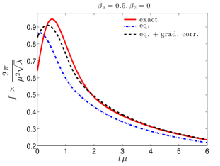
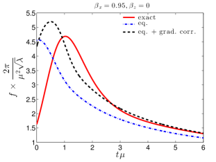
Figure 1: Actual drag force (red curves) from Ref. Chesler:2013cqa on a heavy quark being dragged with $\beta_{z}=0$ and $\beta_{x}=0.5$ (left panel) or $\beta_{x}=0.95$ (right panel) through the debris produced in the collision of two sheets of energy. We compare the actual drag force to the zeroth order calculation (blue dot-dashed curve) which neglects the effects of fluid gradients and our calculation in which the effects of fluid gradients are included up to first order (black dashed curves). At late times, when the fluid has hydrodynamized, the gradient corrections included in the black dashed curves yield a much better description of the full result.

In Fig. 1 we plot the drag force on a quark moving in the $x$-direction, perpendicular to the “beam” direction and therefore perpendicular to the direction of motion of the fluid, with $\beta_{x}=0.5$ and $\beta_{x}=0.95$. The red curves show the drag force obtained from the full gravitational calculation of Ref. Chesler:2013cqa , without any expansion in gradients. The blue dot-dashed curves, which were also obtained in Ref. Chesler:2013cqa , so what the drag force would be at each instant in time in a static homogeneous fluid in thermal equilibrium with the same energy density as the actual fluid has at that instant in time at the location of the quark. An equivalent description of these curves, which are obtained from our expression (42) that is zeroth order in fluid gradients, is that they show what the drag force would be if we neglect all effects of the spatial gradients and variation in time of the fluid at the location of the quark. The black dashed curves show how the drag force changes when we start with the blue dot-dashed curves and add the results of our calculation (65) of the first-order effects of fluid gradients on the drag force. Using the operational definition of the hydrodynamization time $t_{\rm hydro}$ introduced in Ref. Chesler:2010bi , namely taking it to be the time after which the transverse and longitudinal pressure agree with those obtained via the hydrodynamic constitutive relations from the energy density and the fluid velocity, in Fig. 1 hydrodynamization time $t_{\rm hydro}\mu=2.8$. We see that after $t_{\rm hydro}$ the black dashed curves are much closer to the full results shown by the red curves than the blue dot-dashed curves are, meaning that adding effects of fluid gradients to first order has resolved most of the discrepancy between the full results and the zeroth order blue dot-dashed curves. This confirms that this discrepancy was due to the effects of the fluid gradients. It is reasonable to guess that if one were to push our calculation to second order in gradients, the agreement would get even better. We leave this to future work.

We have also checked that the criteria (52) are well satisfied, by more than a factor of two in fact, at all times after $t_{\rm hydro}$ even for $\beta_{x}=0.95$, namely for $\gamma=3.2$. Throughout, we will only show results for cases in which these criteria are satisfied by a large margin.

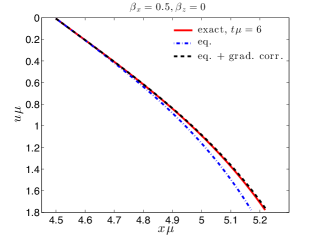
Figure 2: Comparison of the profile of the string trailing “down” into the bulk from the heavy quark moving with $\vec{\beta}=(0.5,0,0)$. The vertical axes show the radial, or holographic, coordinate $u=1/r$, meaning that the AdS boundary at $r=\infty$ is at $u=0$, at the top of the figures. The horizontal axes show $x$; the quark and hence its string is moving to the right. The curves show the shape of the string at a fixed Eddington-Finkelstein time $t$. The left panel shows the string at three times, $t\mu=-3,3$ and 6. The right panel zooms in at $t\mu=6$. In all cases, the solid curve shows the string profile obtained from the full gravitational calculation in Ref. Chesler:2013cqa , the blue dot-dashed curve shows the string profile (18) as it would be at that instant in time $t$ if gradients in the fluid were neglected, and the black dashed curve shows the string profile (28) including the effects of fluid gradients to first order.

To get further intuition, in Fig. 2 we investigate the shapes of the string hanging “down” into the gravitational spacetime from the heavy quark in the calculation of the drag force shown in the left panel of Fig. 1. Each string profile is plotted at fixed Eddington-Finkelstein time $t\mu$ as a function of the inverse radial coordinate $u=1/r$. The solid curves are the exact string profiles at three times, obtained numerically in the gravitational calculation of Ref. Chesler:2013cqa . The blue dot-dashed curves are zeroth order in fluid gradients: they show the shape (18) that the string would have in a static, spatially homogeneous, equilibrium fluid with the same energy density as that at the location of the heavy quark. The black dashed curves are obtained by integrating $\partial_{\sigma}\vec{g}$ in the fluid rest frame, i.e., Eqs. (29). In a case like those we shall turn to below, where the lab frame is not the same as the fluid rest frame, we would then boost the string profile from the fluid rest frame back to the lab frame. We see from Fig. 2 that including the effects of fluid gradients on the string profile to first order yields a much better description of the actual string profile, just as for the drag force itself.

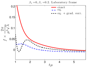
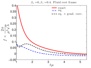
Figure 3: As in Fig. 1, except that here the quark has zero velocity in the direction perpendicular to the motion of the fluid and is moving only in the $z$-direction. In the left panel, $\beta_{z}=0.2$ and in the right panel $\beta_{z}=0.4$. We have shown the left panel in the laboratory frame while in the right panel at each time $t$ we have boosted to the frame in which the fluid is at rest at the location of the quark. As in Fig. 1, we show the exact results for the drag force obtained in Ref. Chesler:2013cqa as well as the zeroth-order approximation (i.e. the drag force in a static homogeneous fluid with the same instantaneous energy density) and the result that we have obtained upon including the effects of fluid gradients to first order.

In Fig. 3 we investigate two cases when the quark is moving with nonzero rapidity, $\beta_{z}\neq 0$. Here we choose to set $\beta_{x}=0$; below we will consider a case when both $\beta_{x}$ and $\beta_{z}$ are nonvanishing. In Fig. 3 we have chosen $\beta_{z}=0.2$ and $\beta_{z}=0.4$. In both cases, and as in Fig. 1, including the first order effects of fluid gradients on the drag force improves the agreement with the exact calculation of the drag force from Ref. Chesler:2013cqa . In Fig. 3 the agreement between the black dashed curves and the solid red curves is worse than in Fig. 1, in fractional terms, but the more striking difference between the two Figures is that the overall magnitude of the forces plotted in Fig. 3 is more than an order of magnitude smaller than the forces in Fig. 1. This can be understood by recalling our results for Bjorken flow, from Section 4.2. If the longitudinal expansion of the fluid produced in the collision that we are analyzing here were boost invariant, our results from Section 4.2 tell us that when we choose $\beta_{z}\neq 0$ and $\beta_{x}=0$ we would find no drag force at all, at zeroth and first order in fluid gradients. The fact that we see a nonzero drag force in Fig. 3 reflects the fact that the expansion of the fluid produced in the collision is not boost invariant. Since at late times the expansion is close to boost invariant Chesler:2013lia , all the forces in Fig. 3 are small in magnitude. Upon realizing this, we also note that the absolute difference between the black dashed and solid curves in Fig. 3 is in fact quite similar to their absolute difference in Fig. 1, meaning that the larger fractional deviation in Fig. 3 is simply an artifact of the smallness of the magnitude of the drag force which is a consequence of the expansion being almost boost invariant.

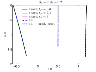
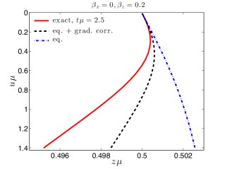
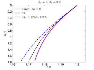
Figure 4: Comparison of the profile of the string trailing “down” into the bulk from the heavy quark moving with $\vec{\beta}=(0,0,0.2)$. The axes are as in Fig. 2. The solid curves show the shape of the string obtained from the full gravitational calculation of Ref. Chesler:2013cqa at three fixed Eddington-Finkelstein times $t$, namely $t\mu=-3,2.5$ and 6. As in Fig. 2, the blue dot-dashed curves show the string profile as if there were no gradients in the fluid and the black dashed curves show the results of this paper, with the effects of fluid gradients taken into account to first order. The lower panels zoom in on the string profiles at $t\mu=2.5$ and 6. We have chosen $t\mu=2.5$ as one of the times at which we illustrate the string profile because it is just before the time $t\mu=2.63$ at which the blue dot-dashed curve in the left panel of Fig. 3 crosses zero, which is to say it is just before the time at which the relative velocity of the quark and the fluid changes sign, meaning that the zeroth-order estimate of the drag force changes sign.

In Fig. 4 we investigate the shapes of the string attached to the heavy quark moving with $\beta_{z}=0.2$ whose drag force is shown in the left panel of Fig. 3 at the three Eddington-Finkelstein times $t\mu=-3,2.5$, and $6$. As in Fig. 2, we see that including the effects of fluid gradients on the string profile to first order improves the description of the exact string profile obtained in Ref. Chesler:2013cqa . Just as when we compared Figs. 1 and 3, when we compare the zoomed-in panels of Fig. 4 to the zoomed-in panel of Fig. 2 we see that the absolute differences between the analytic results to first order in fluid gradients (black dashed curves) and the full results obtained numerically (solid curves) are comparable, although the fractional deviations look greater in Fig. 4.

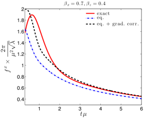
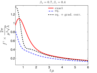
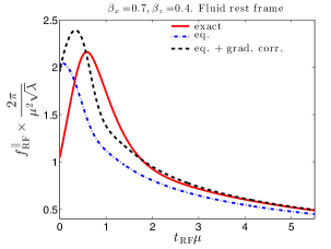
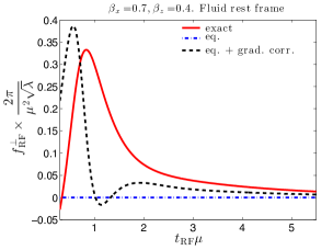
Figure 5: As in Fig. 1, but the case when quark is moving with velocity $\vec{\beta}=(0.7,0,0.4)$, meaning $\beta_{x}=0.7$ perpendicular to the collision direction and $\beta_{z}=0.4$ along the collision axis. The upper two panels show the $x$- and $z$-components (top-left and top-right panels, respectively) of the drag force as seen in the “laboratory frame”, which is to say the center-of-mass frame for the collision. In the lower two panels, we boost to the frame in which the fluid at the location of the heavy quark is at rest. And, instead of showing the $x$- and $z$-components of the drag force in this frame, we show the components of the force in the directions parallel to (bottom-left panel) and perpendicular to (bottom-right panel) the direction of motion of the quark in the local fluid rest frame. In all the panels, the drag force with fluid gradient corrections included to first order (black dashed curve) gives a better description of the full drag force (red curve) than does the zeroth-order drag force with fluid gradients neglected.

We have chosen $t\mu=2.5$ as one of the times at which we illustrate the string profile in Fig. 4 because it is close to the time $t\mu=2.63$ at which the velocity of the fluid at the location of the quark, $v_{z}$, goes from below $0.2$ to above $0.2$, meaning that the relative velocity of the quark and the fluid changes sign at that time. At $t\mu=2.63$, the zeroth-order approximation to the drag force therefore changes sign, as seen in the blue dot-dashed curve in the left panel of Fig. 3. We see that this change is also reflected in the string profile: at $t\mu=2.63$, the string would be hanging straight down from the quark at the boundary; earlier, it angles to the right; later, it angles to the left. We see that at $t\mu=2.5$ the orientation of the string has already changed deeper within the bulk and the change in orientation is about to reach the boundary. Note that the orientation of the string at the boundary suffices to determine the sign of the drag force only to zeroth order. Once the effects of fluid gradients are included, the drag force at time $t$ depends on how the string is moving as well as on the orientation of the string Chesler:2013cqa . We see in the left panel of Fig. 3 that the drag force including effects of fluid gradients to first order (black dashed curve) and the full drag force (red curve) change sign only considerably later than $t\mu=2.63$. Starting at $t\mu=2.63$, when the relative direction of the fluid flow and the quark changes, we have a period of time when the drag force exerted by the fluid on the quark points in the same direction as the velocity of the quark, an effect that was highlighted in Ref. Chesler:2013cqa . We now see from the black dashed curve that this effect can be accounted for qualitatively by the effects of fluid gradients to first order.

The $t\mu=2.5$ panel of Fig. 4 is also interesting insofar as it shows an example where although the difference between the zeroth order string profile and the full string profile is small in magnitude these two profiles have qualitatively different shapes, and we see the first order effects of gradients doing the job of turning the blue dot-dashed curve into a black dashed curve that looks much more like the red solid curve.

Finally, in Fig. 5 we show the results of our calculation of the effects of fluid gradients to first order on the drag force needed to move a heavy quark along a trajectory with both $\beta_{x}\neq 0$ and $\beta_{z}\neq 0$. The message from the upper two panels is much the same as what we have already learned from Fig. 1. In the lower two panels, at each time we boost to a frame in which the fluid at the location of the heavy quark is instantaneously at rest. In this frame, the heavy quark is of course still moving, with a substantial velocity in the $x$-direction and some velocity in the $z$-direction. We have chosen to plot the components of the drag force in this frame in the directions parallel to and perpendicular to the direction of motion of the quark in this frame. The bottom-left plot is, again, similar to other plots that we have seen. The bottom-right plot is, however, of particular interest because the blue dot-dashed curve in this plot vanishes: in the local fluid rest frame to zeroth order in gradients the drag force must be parallel to the direction of motion of the heavy quark; without the effects of fluid gradients, there can be no perpendicular component. We have also seen in Section 4.2 that if the expansion were boost invariant then in the local fluid rest frame the drag force on the heavy quark would still act parallel to the direction of motion of the heavy quark even when the effects of fluid gradients are taken into account to first order. Therefore, the fact that the black dashed curve in the bottom-right panel of Fig. 5 is nonzero is a direct manifestation of the effects of fluid gradients and of the fact that the expanding fluid produced in the collision of the two sheets of energy is not boost invariant. The magnitude of the force described by this curve is small, since the expansion is close to boost invariant, but it is nonzero. We also see that the first order effects of fluid gradients push the black dashed curve toward the full result, shown as usual by the red curve.

We conclude from the investigations that we have reported in this section that the discrepancies observed in Ref. Chesler:2013cqa between the actual drag force on a heavy quark being pulled through the matter produced in the collision of sheets of energy and the drag force that would have been obtained in an static, homogeneous, plasma with the same energy density is indeed due to the effects of spatial gradients in, and time derivatives of, the fluid on the drag force. Evaluating these effects to first order in the fluid gradients explain all the qualitative aspects of the discrepancies found in Ref. Chesler:2013cqa and do a reasonable job even at the quantitative level.

5 Future directions

In (65) we have derived a general expression for the drag force needed to pull a heavy quark through a dynamic fluid, flowing in some arbitrary fashion described by hydrodynamics, to first order in the gradients and time derivatives of the fluid velocity. We have applied this result to heavy quarks moving through a fluid that is expanding according to Bjorken flow and to heavy quarks moving through the expanding and cooling liquid produced in a collision of sheets of energy in strongly coupled ${\cal N}=4$ SYM theory. Future directions include applying (65) to heavy quarks moving through strongly coupled plasma whose dynamics is described by other hydrodynamic solutions, for example including transverse expansion. It would also be interesting, and challenging, to extend (65) to second order in fluid gradients. Doing so could clarify how the drag force behaves in the large $\gamma$ limit in the case where, as we have done, one assumes that the quark mass $M\rightarrow\infty$ limit has been taken first. We have seen that in this regime when (52) is not satisfied the first order contributions of the fluid gradients dominate over the zeroth order drag force, which motivates an evaluation of the magnitude of the second order contributions. Considering the effects of fluid gradients on a finite-mass quark at a large enough $\gamma$ that (53) is not satisfied would, however, require a different calculation entirely. The right starting point for this would be an analysis of the rate of energy loss and transverse momentum broadening of a light quark in a dynamic strongly coupled fluid, including the effects of fluid gradients. Other interesting directions would include investigating how gradients in the fluid affect the emission of photons and dileptons or the screening of the attraction between a heavy quark and antiquark, and hence how they affect the binding or dissociation of quarkonia. We leave the holographic calculation of the effects of fluid gradients on these and other probes of the strongly coupled fluid to future work.

- (1) M. Gyulassy and X.-N. Wang, Nucl. Phys. B 420, 583 (1994) [nucl-th/9306003].
- (2) R. Baier, Y. L. Dokshitzer, A. H. Mueller, S. Peigne and D. Schiff, Nucl. Phys. B 483, 291 (1997) [hep-ph/9607355].
- (3) R. Baier, Y. L. Dokshitzer, A. H. Mueller, S. Peigne and D. Schiff, Nucl. Phys. B 484, 265 (1997) [hep-ph/9608322].
- (4) B. G. Zakharov, JETP Lett. 65, 615 (1997) [hep-ph/9704255].
- (5) Y. L. Dokshitzer and D. E. Kharzeev, Phys. Lett. B 519, 199 (2001) [hep-ph/0106202].
- (6) J. M. Maldacena, Adv. Theor. Math. Phys. 2, 231 (1998) [hep-th/9711200].
- (7) E. Witten, Adv. Theor. Math. Phys. 2, 253 (1998) [hep-th/9802150].
- (8) A. Karch and E. Katz, JHEP 0206, 043 (2002) [hep-th/0205236].
- (9) C. P. Herzog, A. Karch, P. Kovtun, C. Kozcaz and L. G. Yaffe, JHEP 0607, 013 (2006) [hep-th/0605158].
- (10) S. S. Gubser, Phys. Rev. D 74, 126005 (2006) [hep-th/0605182].
- (11) J. Casalderrey-Solana and D. Teaney, Phys. Rev. D 74, 085012 (2006) [hep-ph/0605199].
- (12) A. Adare et al. [PHENIX Collaboration], Phys. Rev. Lett. 98, 172301 (2007) [nucl-ex/0611018].
- (13) J. Casalderrey-Solana, H. Liu, D. Mateos, K. Rajagopal and U. A. Wiedemann, arXiv:1101.0618 [hep-th].
- (14) C. P. Herzog, JHEP 0609, 032 (2006) [hep-th/0605191].
- (15) E. Caceres and A. Guijosa, JHEP 0611, 077 (2006) [hep-th/0605235].
- (16) E. Caceres and A. Guijosa, JHEP 0612, 068 (2006) [hep-th/0606134].
- (17) T. Matsuo, D. Tomino and W. -Y. Wen, JHEP 0610, 055 (2006) [hep-th/0607178].
- (18) E. Nakano, S. Teraguchi and W. -Y. Wen, Phys. Rev. D 75, 085016 (2007) [hep-ph/0608274].
- (19) P. Talavera, JHEP 0701, 086 (2007) [hep-th/0610179].
- (20) S. S. Gubser, Phys. Rev. D 76, 126003 (2007) [hep-th/0611272].
- (21) G. Bertoldi, F. Bigazzi, A. L. Cotrone and J. D. Edelstein, Phys. Rev. D 76, 065007 (2007) [hep-th/0702225].
- (22) H. Liu, K. Rajagopal and Y. Shi, JHEP 0808, 048 (2008) [arXiv:0803.3214 [hep-ph]].
- (23) U. Gursoy, E. Kiritsis, G. Michalogiorgakis and F. Nitti, JHEP 0912, 056 (2009) [arXiv:0906.1890 [hep-ph]].
- (24) C. Hoyos-Badajoz, JHEP 0909, 068 (2009) [arXiv:0907.5036 [hep-th]].
- (25) F. Bigazzi, A. L. Cotrone, J. Mas, A. Paredes, A. V. Ramallo and J. Tarrio, JHEP 0911, 117 (2009) [arXiv:0909.2865 [hep-th]].
- (26) A. Nata Atmaja and K. Schalm, JHEP 1104, 070 (2011) [arXiv:1012.3800 [hep-th]].
- (27) M. Chernicoff, D. Fernandez, D. Mateos and D. Trancanelli, JHEP 1208, 100 (2012) [arXiv:1202.3696 [hep-th]].
- (28) K. B. Fadafan and H. Soltanpanahi, JHEP 1210, 085 (2012) [arXiv:1206.2271 [hep-th]].
- (29) P. M. Chesler, M. Lekaveckas and K. Rajagopal, JHEP 1310, 013 (2013) [arXiv:1306.0564 [hep-ph]].
- (30) P. M. Chesler and L. G. Yaffe, Phys. Rev. Lett. 106, 021601 (2011) [arXiv:1011.3562 [hep-th]].
- (31) J. Casalderrey-Solana, M. P. Heller, D. Mateos and W. van der Schee, arXiv:1305.4919 [hep-th].
- (32) P. M. Chesler and L. G. Yaffe, arXiv:1309.1439 [hep-th].
- (33) S. Bhattacharyya, V. E. Hubeny, S. Minwalla and M. Rangamani, JHEP 0802, 045 (2008) [arXiv:0712.2456 [hep-th]].
- (34) G. Policastro, D. T. Son and A. O. Starinets, Phys. Rev. Lett. 87, 081601 (2001) [hep-th/0104066].
- (35) P. Kovtun, D. T. Son and A. O. Starinets, JHEP 0310, 064 (2003) [hep-th/0309213].
- (36) A. Buchel and J. T. Liu, Phys. Rev. Lett. 93, 090602 (2004) [hep-th/0311175].
- (37) P. Kovtun, D. T. Son and A. O. Starinets, Phys. Rev. Lett. 94, 111601 (2005) [hep-th/0405231].
- (38) S. Bhattacharyya, V. E. Hubeny, R. Loganayagam, G. Mandal, S. Minwalla, T. Morita, M. Rangamani and H. S. Reall, JHEP 0806, 055 (2008) [arXiv:0803.2526 [hep-th]].
- (39) N. Abbasi and A. Davody, JHEP 1206, 065 (2012) [arXiv:1202.2737 [hep-th]].
- (40) N. Abbasi and A. Davody, arXiv:1310.4105 [hep-th].
- (41) H. Liu, K. Rajagopal and U. A. Wiedemann, JHEP 0703, 066 (2007) [hep-ph/0612168].
- (42) J. Casalderrey-Solana and D. Teaney, JHEP 0704, 039 (2007) [hep-th/0701123].
- (43) A. Guijosa and J. F. Pedraza, JHEP 1105, 108 (2011) [arXiv:1102.4893 [hep-th]].
- (44) J. D. Bjorken, Phys. Rev. D 27, 140 (1983).
- (45) R. Baier, P. Romatschke, D. T. Son, A. O. Starinets and M. A. Stephanov, JHEP 0804, 100 (2008) [arXiv:0712.2451 [hep-th]].
- (46) P. M. Chesler and L. G. Yaffe, Phys. Rev. D 82, 026006 (2010) [arXiv:0906.4426 [hep-th]].
- (47) R. A. Janik and R. B. Peschanski, Phys. Rev. D 73, 045013 (2006) [hep-th/0512162].
- (48) G. C. Giecold, JHEP 0906, 002 (2009) [arXiv:0904.1874 [hep-th]].
- (49) A. Stoffers and I. Zahed, Phys. Rev. C 86, 054905 (2012) [arXiv:1110.2943 [hep-th]].
- (50) S. S. Gubser, Phys. Rev. D 82, 085027 (2010) [arXiv:1006.0006 [hep-th]].
- (51) S. S. Gubser, Phys. Rev. C 87, 014909 (2013) [arXiv:1210.4181 [hep-th]].