The Arnold-Tongue of Coupled Acoustic Oscillators

Abstract

Wind-driven sound generation is a source of anger and pleasure, depending on the situation: airframe and car noise, or combustion noise are some of the most disturbing environmental pollutions, whereas musical instruments are sources of joy. We present an experiment on two coupled sound sources -organ pipes- together with a theoretical model which takes into account the underlying physics. Our focus is the Arnold tongue which quantitatively captures the interaction of the sound sources, we obtain very good agreement of model and experiment, the results are supported by very detailed CFD computations.

Understanding wind-driven sound generation and -radiation is of high importance in many everyday situations, as noise from moving objects, whistling noise, combustion noise, industrial noise, or -to name a beautiful example- musical instruments. Models, which describe such systems as self-sustained oscillators have been developed Abel et al. (2009, 2006), and put these systems in a very general perspective with the results having impact on synchronization community, including biosystems, lasers, mechanics, or social systems Pikovsky et al. (2001). In a previous publication, an organ pipe, externally driven by a loudspeaker at a fixed position, was investigated with focus on the detuning with the coupling varied by the speakers amplitude Abel et al. (2009). However, for real aeroacoustical systems synchronization changes drastically with distance, or coupling, as we demonstrate hereafter. Here, we focus on the coupling mechanism by analyzing experimental data in comparison with theoretical modeling. Results are supported by detailed simulations of the compressible Navier-Stokes equations. We present results on two coupled pipes, based on a refined experiment with detailed measurement of the phase relation. As in previous setups, we record the interfered signal at one microphone and analyze the synchronization regions and the measured Arnold tongue.

In contrast to a simple model with direct coupling, we find an Arnold tongue which shows strongly nonlinear behavior. This is typical for systems with nontrivial coupling. Consequently, we focus on the coupling mechanism: we model the system with an empirical factor that considers the coupling between the sound-generating wind field, and the wave propagation, which in turn involves $1/r$ attenuation of the sound field and a delay term which reflects the time delayed coupling of the field generated at the place of one pipe with the other one at a different place. The results of model and measurement coincide very well in the far field, in the near field the sound propagation rather follows an $1/r^{2}$ law such that deviations occur naturally.

Let us briefly sketch the typical functioning of an organ pipe. Energy is supplied steadily by the wind system through the pipe foot and establishes a turbulent vortex street. Each time a vortex detaches, a pressure fluctuation enters the resonator, inside which characteristic waves are selected (resonator), and radiated at the pipe mouth by an oscillating air-sheet Fabre and Hirschberg (2000); Fabre et al. (1996) (oscillator). Inside the resonator energy is dissipated. The coupling of an external acoustical field can be described by a (nonlinear) acoustical admittance Thwaites and Fletcher (1983). As argumented in Abel et al. (2009), the air sheet is the source of sound radiation, and the measurement at the microphone can be taken as the state of the oscillator.

The setup was analogous to the one described in Abel et al. (2006), however with smaller, and thus higher-pitched, pipes. The measurements were carried out on a miniature organ especially made by Alexander Schuke GmbH Sch (2004). The air-supply was connected via a mechanical regulating-valve to a wind-belt, the two pipes were joined directly to the wind-belt by flexible tubes. Whereas in Abel et al. (2006), the pipes stood side-by-side, here, both were mounted on a horizontal bar, along which their position, i.e. their mutual distance, was controlled, cf. Fig. 1. Another difference was the size: here, we used smaller, stopped pipes, tuned at $720\usk\mathrm{Hz}$, with a more suitable wavelength $\lambda\simeq 0.48\usk\mathrm{m}$ for distance variation, details on the pipe geometry are given in the supplement.

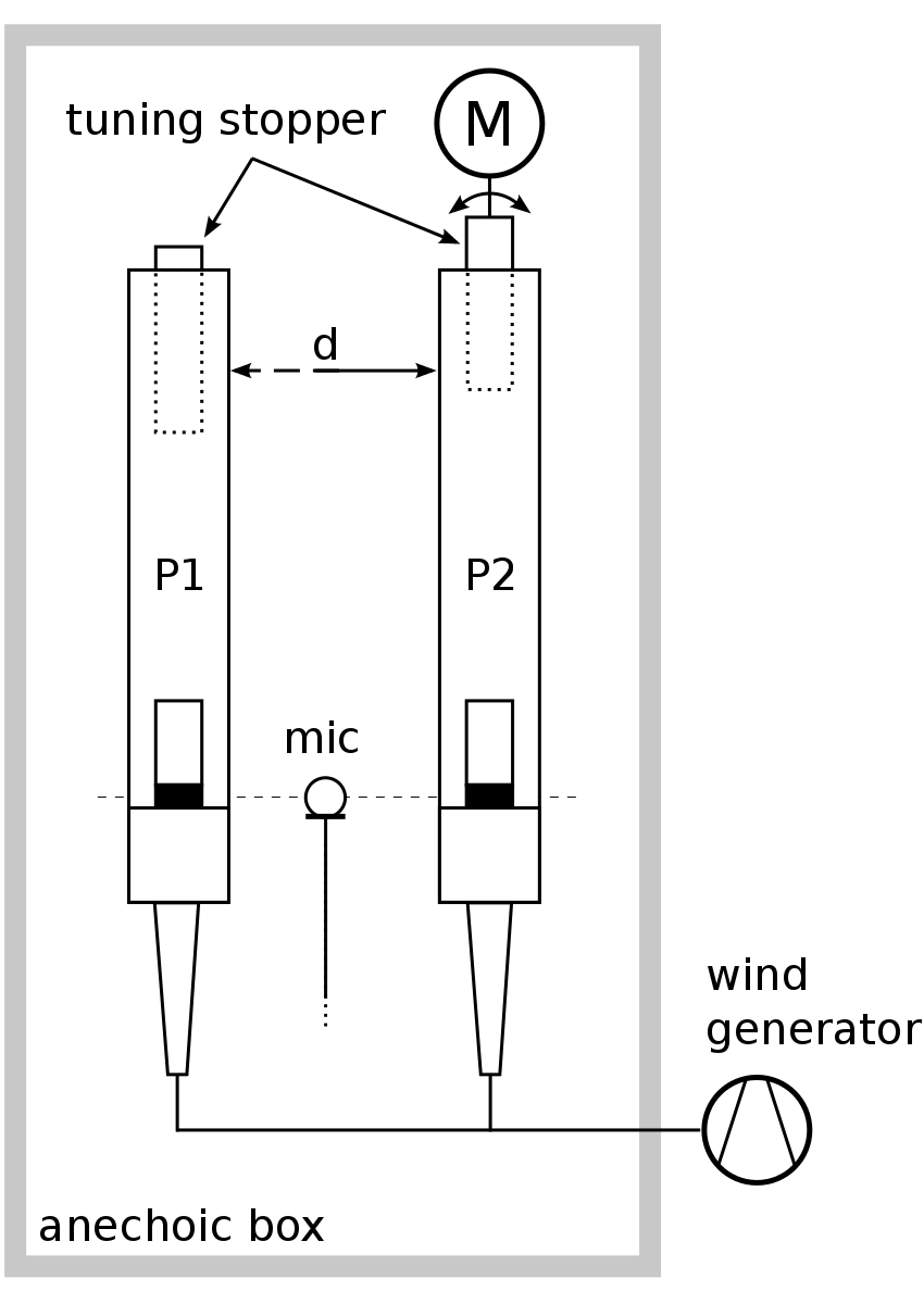
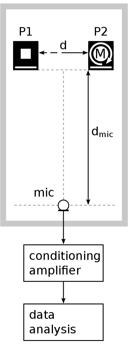
Figure 1: Experimental setup. (a) front view: P1, and P2: tunable organ pipes. Both are connected by flexible tubes to a wind generator, positioned outside the anechoic box, sketched as the thick gray frame. The identically constructed, stopped pipes were mounted on a common bar, their distance d could be varied. The frequency $f_{2}$ of $P2$ was tuned by the step motor (M), in steps of $0.5\usk\mathrm{Hz}$ erh ht. (b) top view: the microphone was positioned at a distance $d_{mic}=1\usk\mathrm{m}$ in the midplane of P1 and P2. Its signal was amplified by a Brüel & Kær Nexus 2690 amplifter and stored for later data analysis.

This allowed us to use of the anechoic chamber of Potsdam University ($B\cdot H\cdot T=1.6\usk\mathrm{m}\cdot 2.0\usk\mathrm{m}\cdot 1.3\usk\mathrm{m}$). During the experiment humidity, temperature, and pressure were monitored and held constant at the normal conditions $L_{h}=20\usk$%, $T_{0}=20\usk\mathrm{\SIUnitSymbolCelsius}$, $p_{0}=1013.25\usk\mathrm{h}\mathrm{Pa}$.

Our main goal was the investigation of the Arnold-tongue, i.e. a scan of the parameter space coupling, $\epsilon$, vs. detuning , $\Delta f$. For the coupling strength, we mounted the pipes $P1$, and $P2$ on a common horizontal bar, along which their mutual distance $d$, was controlled (Fig. 1). To vary the second important parameter, the frequency detuning $\Delta f$, $P1$ was tuned at $f_{P1}=720\usk\mathrm{Hz}$, while $f_{P2}$ was varied by a step motor in the range of $700-740\usk\mathrm{Hz}$, and $680-760\usk\mathrm{Hz}$ for large and small distances, respectively (small distances correspond to large coupling and vice versa). The pipes were well-tuned independent on eachother before coupling them.

To explore parameter space, the pipes were positioned at the distances $1,10,30,50,75,100,200,300$, and $400\usk\mathrm{m}\mathrm{m}$. For each distance the frequency was varied as described above in steps of $0.5\usk\mathrm{Hz}$, for details see sup . The acoustic signal was measured by a Brüel & Kær 4191 condenser microphone at $d_{mic}=1\usk\mathrm{m}$ distance, from the pipes midpoint, at the centerline between the sound sources cf. Fig. 1, which satisfies the farfield condition $d>\lambda$. The sampling rate was $f_{s}=44.1\usk\mathrm{k}\mathrm{Hz}$ with a resolution of $16\usk$bit. The data analysis and signal processing was programmed using MATLAB^® .

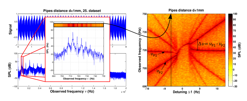
Figure 2: From signal to synchronization plot: Left: the signal is Fourier-transformed, the resulting spectrum is color coded, and the maxima are determined. Right: For each detuning $\Delta f$ we obtain such a bar; further we combine such bars for each distance $d$ and obtain the colorful plot on the right, here for $d=1\usk\mathrm{m}\mathrm{m}$. The maxima give the measured frequency difference $\Delta\nu$, which vanishes for synchronized behavior. The amplitude of the measured signal achieves maximum for in-phase and minimum for anti-phase synchronization.

Data Analysis: A synchronization plot is generated by the procedure illustrated in Fig. 2: We are interested in the freqency difference and amplitude measured at the microphone, since this gives us information on the relative phases $\phi_{01},\phi_{02}$ of the two pipes, which in turn yield negative or positive interference, causing a mutual cancellation or amplification Stanzial et al. (2001); Angster et al. (1993); Abel et al. (2006, 2009). To obtain a synchronization plot $\Delta\nu$ vs. $\Delta f$, we first Fourier transform the signal (Fig. 2, left), and consider the region $690\usk\mathrm{Hz}\leq\nu_{P1,P2}\leq 750\usk\mathrm{Hz}$. This part of the spectrum is turned into color-coded SPL stripe. We collect these stripes for each detuning and obtain a spectral plot $\nu_{meas}$ vs. $\Delta f$, with either several or one vertical frequencies corresponding to (non)synchronized behavior. The amplitude allows to infer the phase relation of the two pipes, cf. Fig. 2, (right), The final synchronization plot is obtained by identifying the two main peaks $\nu_{1}$ and $\nu_{2}$ which yield $\Delta\nu$. This procedure is repeated for every distance, the resulting curves are plotted in Fig. 3.

In addition to the phases, we plot the SPL at the microphone (Fig. 3, b) From its minimum we obtain the phase difference between the two pipes. Within the error bars, the plot confirms the idea that the interference is as for two harmonic oscillators with phase difrerence $\Delta\Phi_{0}$ at the microphone.

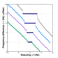
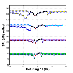
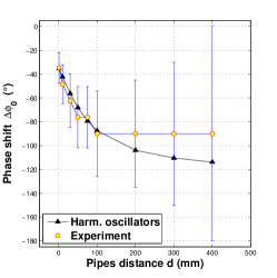
Figure 3: Left:Synchronisation plateau, for good for 4 exemplary distances $d=100,50,10$ and $1\usk\mathrm{m}\mathrm{m}$. The y-axis is plotted for $d=100\usk\mathrm{m}\mathrm{m}$. For the distances $d=50,10$ and $1\usk\mathrm{m}\mathrm{m}$ an offset of $5,10$ and $15\usk\mathrm{Hz}$ is added to separate the curves. All nine figures are found in sup . Right: Analogous plot for the peak amplitudes of the two pipes. The y-axis is plotted for $d=100\usk\mathrm{m}\mathrm{m}$. For the distances $d=50,10$ and $1\usk\mathrm{m}\mathrm{m}$ an offset of $50,100$ and $150\usk\mathrm{Hz}$ is added to separate the curves. The synchronisation regions are labeled black. One recognizes a shift of the relative phases $\Delta\Phi_{0}$ while the distance is increased. The signal recorded at a microphone in the far field coincides nicely with the signal one would obtain for two harmonically oscillating sources at the position of the two pipes. The vertical bars denote the errors which follow from the frequency discretization.

Given one such curve for each distance, we retrieve the Arnold tongue in $(d,\Delta f)$-space. We recognize an Arnold tongue with strongly curved boundaries (Fig. 4), typical for real experiments with delay and complicated couplings Flunkert et al. (2013). In order to understand this behaviour from physical reasoning, we now develop a model consistent with aeroacoustics and nonlinear dynamics.

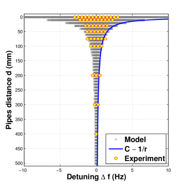
Figure 4: Arnold tongue for two coupled organ pipes. Circles: The horizontal error bars correspond to the frequency resolution which sets the accuracy for the detection of the transition to synchronization with changing detuning. The stars correspond to results for the model, given in Eq.2. The ordinate is plotted top-down, because the coupling decreases with increasing distance. The straight line corresponds to the expected coupling decrease with $1/d$. Experiment and model agree very well.

In order to understand the observed behaviour we have to recall that our observed system obeys the compressible Navier-Stokes-Equation with suitable boundary conditions. The signal measured is the acoustic field (not the aerodynamic wind field), at the microphone position. In order to reproduce the measured curve, we have to i) find a good model for a single organ pipe as a self-excited oscillator, ii) find a model for the emission of acoustical waves from an oscillating jet, iii) describe the propagation from pipe to pipe iv) find a model for the coupling of the acoustic field - the one emitted by the partner pipe- to the jet of a pipe. In the following we describe the situation that sound emitted at $x_{2}$ by pipe 2 influences the jet at $x_{1}$, pipe 1. Further, we understand the locations in a coarse-grained sense, i.e. the whole jet is located at $x_{1}$, defined appropriately, e.g. as the mean jet position.

i) Single organ pipe. A self-sustained oscillator consists of an oscillating unit, and energy source and sink, both possibly nonlinear. In our case, the oscillating unit is the jet, which exits from the pipe mouth and can be described by its displacement normal to the pipe longer axis. Its frequency is set by the resonator: initially, the jet impinges on the labium and a turbulent vortex street develops.

Each time a vortex detaches a pressure wave travels upwards inside the resonator, is reflected at the closed end and travels back to hit the labium after the period $T=c/(\lambda/4)$ with $T$, with $c$ the speed of sound and $\lambda$ the wavelength. The high pressure in turn triggers the detachment of the next vortex, and very quickly a regular oscillation is established Howe (1975); Fabre et al. (1996). Of course, this is an idealized description and the true 3D pipe shows some quite complicated additional effects; the main physics, however, is covered well by this picture; this is supported by many numerical runs, cf. sup . The energy is supplied by the pressure difference at the jet outlet, such that the oscillator carries its own power supply as the mean jet velocity. To first order the period depends linearly on the jet velocity. The energy sink is here twofold: nonlinear energy dissipation inside the resonator and at the walls, and radiation of an acoustical wave. From Abel et al. (2009) we know that empirically one finds an excellent match for a van-der-Pol oscillator with additional weak higher-order nonlinear damping.

ii) The jet at $x_{2}$ emits a (sound) velocity wave, which is related to pressure by $p_{2}=Z\,v\,A_{jet}$ with $Z$ the acoustical impedance at the jet. This is very hard to determine from first principles. Since the jet is an extended source where each point emits sound, a coarse-grained description must involve spatio-temporal averaging over the source region and long enough time, this is subject of future numerical work. Here, we assume no phase shift and direct proportionality of emitted sound and jet displacement with an empirical factor $C_{em}$.

iii) A spherical (pressure) wave, emitted at $x_{2}$ with amplitude $p_{2}$ and frequency $f_{2}$ propagates to $x_{1}$ according to $p_{2}(x_{1},t_{1})=\frac{p_{2}(x_{2},t_{2})}{d}\cdot e^{i(k_{2}d-\omega_{2}\tau)}$, with $d=x_{1}-x_{2}$, and $\tau=t_{1}-t_{2}$ Ingard (2008).

iv) The integral force on the jet region at $x_{1}$ is $F_{in}=C_{in}p_{2}(x_{1},t_{1})\cdot A_{jet}$, with $p_{2}$ the sound emitted by pipe 2, and $A_{jet}$ the area covered by the jet.

Alltogether, we obtain for the force from pipe 2 on jet 1: $F_{21}=C_{in}\frac{p_{2}(x_{2},t_{2})}{d}\cdot e^{i(k_{2}d-\omega_{2}\tau)}C_{em}$. As usual, there is a difference between near field and far field in that pressure and velocity show the characteristic phase difference of $\pi/2$ or 0 and $1/d$, or $1/d^{2}$, respectively.

For a complete model, we combine i)-iv), to obtain a model for the displacement of the jet, $\xi$:

$$\ddot{\xi}_{1}-\mu_{1}(1-\beta_{1}\xi_{1}^{2})\dot{\xi}_{1}+\omega_{01}^{2}\xi_{1} = C_{1}\dot{\xi}_{2}$$ (1)

$$\ddot{\xi}_{2}-\mu_{2}(1-\beta_{2}\xi_{2}^{2})\dot{\xi}_{2}+\omega_{02}^{2}\xi_{2} = C_{2}\dot{\xi}_{1}\,,$$ (2)

with $\mu_{i}$ the energy supply by velocity $\dot{\xi}_{i}$, $\beta_{i}$ the nonlinear damping, $\omega_{0i}$ the individual angular frequency, these terms characterize the individual pipes ($i=1,2$). The coupling is modeled by the coefficients $C_{i}$ with $C_{i}=C_{i,em}\cdot C_{i,trans}\cdot C_{i,in}$. where $C_{1}$, $C_{2}$ model the sound-fluid interaction. A more realistic model needs to include the frequency shift during wave propagation, this is subject of ongoing research.

How does the coupling influence the Arnold tongue? We integrated Eq. 2 numerically using odeint Ahnert and Mulansky (2011). We do assume that both pipes stay at a fixed phase relation after some transients, such that we neglect the oscillation $e^{i\omega t}$, and the relative phase change during propagation is captured by the term $e^{-ik}$. As a result, we obtain an Arnold tonge which coincides very well with the experimental data, cf. Fig. 4. At a closer look, one finds deviations for high coupling (small distance). This is explained by the fact that in the acoustic near field the $1/r$ law does not hold, and rather a $1/r^{2}$ behavior is expected. Since the range of scales is too small, one cannot clearly make out a power-law, cf.sup .

Summary: We investigated an improved experimental setup of two coupled wind-driven sound sources. As well controlled realization, we used organ pipes. The model for a single pipe presented in Abel et al. (2009) is consistent with pipes of various dimensions, indicating that our results can be transferred to other wind-driven oscillatory systems. Furthermore, we developed a model for the coupling of two sound sources (two jets) by modeling the coupling sound-jet with an empirical factor, the sound wave is modeled as a monopole, whose propagator includes attenuation with inverse distance. The coupling into the jet is again modeled by a phase shift and an empirical factor.

The Arnold tongue measured shows a clear curvature which can be explained by the above model in very good coincidence with the experiment in the far field. This has been validated by numerical integration of the two coupled ODEs. In the near field, the sound field is highly angle-dependent and in general decays with squared inverse distance. This is again confirmed by the comparison of numerical and experimental results.

We see our results in a much more general context than musical acoustics: on one hand, we have investigated one aspect of the fundamental question of sound emission by a turbulent jet. On the other hand we have demonstrated how powerful the concept of synchronization can be applied even for 3D systems with turbulent behavior. Indeed, we are running an experiment on coupled Rijke tubes, which are an excellent example for flame-induced combustion noise. Eventually, we have contributed to improve the understanding of one of the most beautiful instruments humans have created - the organ.

References

- Abel et al. [2009] M. Abel, K. Ahnert, and S. Bergweiler. Synchronization of sound sources. Phys. Rev. Lett., 103(114301), 2009.
- Abel et al. [2006] M. Abel, S. Bergweiler, and R. Gerhard-Multhaupt. Synchronization of organ pipes by means of air flow coupling: experimental observations and modeling. J. Acoust. Soc. Am., 119(4):2467 – 2475, 2006.
- Pikovsky et al. [2001] A. Pikovsky, M. Rosenblum, and J. Kurths. Synchronization—A Universal Concept in Nonlinear Science. Springer, Berlin, 2001.
- Fabre and Hirschberg [2000] B. Fabre and A. Hirschberg. Physical modeling of flue instruments: A review of lumped models. Acustica - Acta Acustica, 86:599–610, 2000.
- Fabre et al. [1996] B. Fabre, A. Hirschberg, and A. P. J. Wijnands. Vortex shedding in steady oscillation of a flue organ pipe. Acustica - Acta Acustica, 82:863–877, 1996.
- Thwaites and Fletcher [1983] S. Thwaites and N.H. Fletcher. Acoustic admittance of organ pipe jets. J. Acoust. Soc. Am., 74:400–408, 1983.
- Sch [2004] Alexander Schuke GmbH, 2004. URL http://www.schuke.com.
- [8] Supplemental information.
- Stanzial et al. [2001] D. Stanzial, D. Bonsi, and D. Gonzales. Nonlinear modelling of the mitnahme-effekt in coupled organ pipes. In International symposium on musical acoustics (ISMA) 2001, Perugia, Italy, pages 333–337, 2001.
- Angster et al. [1993] Judith Angster, József Angster, and András Miklós. Coupling between simultaneously sounded organ pipes. AES Preprint 94th Convention Berlin 1993, March 1993.
- Flunkert et al. [2013] Valentin Flunkert, Ingo Fischer, and Eckehard Schöll. Dynamics, control and information in delay-coupled systems: an overview. Phil. Trans. R. Soc. A., 371:20120465, 2013. doi: 10.1098/rsta.2012.0465.
- Howe [1975] M. S. Howe. Contribution to the theory of aerodynamic sound, with application to excess jet noise and theory of the flute. J. Fluid Mech., 71:625–673, 1975.
- Ingard [2008] Uno Ingard. Acoustics. Infinity Science Press, Hingham, MA, 2008.
- Ahnert and Mulansky [2011] Karsten Ahnert and Mario Mulansky. Odeint - solving ordinary differential equations in c++. In AIP Conf. Proc., volume 1389, page 1586. AIP, 2011.