Metal-Poor Stars Observed with the Magellan Telescope. II.
Discovery of Four Stars with [Fe/H] $\leq-3.5$

Abstract

We report on the discovery of seven low-metallicity stars selected from the Hamburg/ESO Survey, six of which are extremely metal-poor ([Fe/H] $\leq-$3.0), with four having [Fe/H] $\leq-$3.5. Chemical abundances or upper limits are derived for these stars based on high-resolution (R $\sim~{}35,000$) Magellan/MIKE spectroscopy, and are in general agreement with those of other very and extremely metal-poor stars reported in the literature. Accurate metallicities and abundance patterns for stars in this metallicity range are of particular importance for studies of the shape of the metallicity distribution function of the Milky Way’s halo system, in particular for probing the nature of its low-metallicity tail. In addition, taking into account suggested evolutionary mixing effects, we find that six of the program stars (with [Fe/H] $\leq-$3.35) possess atmospheres that were likely originally enriched in carbon, relative to iron, during their main-sequence phases. These stars do not exhibit over-abundances of their $s$-process elements, and hence may be additional examples of the so-called CEMP-no class of objects.

1. Introduction

The very metal-poor (VMP; [Fe/H] $\leq-2.0$) and extremely metal-poor (EMP; [Fe/H] $\leq-3.0$) stars provide a direct view of Galactic chemical and dynamical evolution; detailed spectroscopic studies of these objects are the best way to identify and distinguish between a number of possible scenarios for the enrichment of early star-forming gas clouds soon after the Big Bang. Thus, over the last 25 years, several large survey efforts were carried out in order to dramatically increase the numbers of VMP and EMP stars known in our galaxy, enabling their further study with high-resolution spectroscopy. Taken together, the early HK survey (Beers et al., 1985, 1992) and the Hamburg/ESO Survey (HES; Wisotzki et al., 1996; Christlieb et al., 2001; Christlieb, 2003; Christlieb et al., 2008) identified several thousand VMP stars (Beers & Christlieb 2005; for a more recent summary of progress, see Frebel & Norris 2011). To date, the two most metal-poor (strictly speaking, most iron-deficient) stars found in the halo of the Galaxy, HE 0107$-$5240 ([Fe/H] = $-$5.2; Christlieb et al., 2002) and HE 1327$-$2326 ([Fe/H] = $-$5.6; Frebel et al., 2005), were first identified from spectroscopic follow-up of candidate VMP/EMP stars in the HES stellar database.

In the past decade, the numbers of metal-poor stars has been further increased, by over an order of magnitude, through the use of medium-resolution spectroscopy carried out during the Sloan Digital Sky Survey (SDSS; York et al., 2000) and the sub-surveys Sloan Extension for Galactic Understanding and Exploration (SEGUE-1; Yanny et al., 2009) and SEGUE-2 (C. Rockosi et al., in preparation), to many tens of thousands of VMP (and on the order of 1000 EMP) stars. Although follow-up high-resolution spectroscopy of likely VMP/EMP stars from SDSS/SEGUE has only recently begun (e.g., Caffau et al., 2011b; Bonifacio et al., 2012; Aoki et al., 2013), the SDSS/SEGUE sample has already resulted in the discovery of several stars in the ultra metal-poor (UMP; [Fe/H] $<-4.0$) range, SDSS J102915$+$172927, with [Fe/H] = $-$4.73 (Caffau et al., 2011a), SDSS J144256$+$253135, with [Fe/H] = $-$4.09 (Caffau et al., 2013), and another star, SDSS J174259$+$253135, for which iron lines could not be measured, but with [Ca/H] $<-4.5$ (Caffau et al., 2013).

There exists a substantial number of published high-resolution studies of stars identified by the above surveys (and others), due to the wealth of information concerning early element production that can be extracted. Examples of these efforts are the “Survey of Proper Motion Stars” series (e.g., Carney et al., 1994), the “First Stars” project (Cayrel et al., 2004; François et al., 2007, among others in the series), the “The 0Z Project” (Cohen et al., 2008, 2011; Cohen et al., 2013), the “Extremely Metal-Poor Stars from SDSS/SEGUE” series (Aoki et al., 2013), and “The Most Metal-Poor Stars” series (Norris et al., 2013a; Yong et al., 2013a), as well as smaller individual samples from Ryan et al. (1991, 1996, 1999), McWilliam et al. (1995), Lai et al. (2008), Hollek et al. (2011), and others. Roederer et al. (2013) describe a high-resolution spectroscopic analysis of some 300 VMP/EMP stars originally identified by the HK Survey. These studies all aim to provide large, homogeneous datasets of metal-poor stars, and to address differences in their chemical abundance patterns at the lowest metallicities. Taking into account the published work that we are aware of, the current total number of EMP stars with available high-resolution spectroscopic determinations is 205. This number drops to 50 for [Fe/H] $<-3.5$, 12 for [Fe/H] $<-4.0$, and only 4 stars observed to date with [Fe/H] $<-4.5$ (Suda et al., 2008; Frebel, 2010; Yong et al., 2013a).

The number of EMP stars with well-determined metallicities also has a direct impact on the observed metallicity distribution function (MDF) for the halo system of the Milky Way. The MDF provides important constraints on the structure and hierarchical assembly history of the Galaxy (see, e.g., Carollo et al., 2007, 2010; Tissera et al., 2010; Beers et al., 2012; McCarthy et al., 2012; Tissera et al., 2012, 2013), on quantities such as the initial mass function and early star-formation rate (see, e.g., Romano et al., 2005; Pols et al., 2012; Chiappini, 2013; Lee et al., 2013; Suda et al., 2013), and on tests of models for Galactic chemical evolution (see e.g., Romano et al., 2005; Chiappini, 2013; Karlsson et al., 2013; Nomoto et al., 2013, and references therein).

Recent studies based on observations of metal-poor giants and main-sequence turnoff stars from the HES (Schörck et al., 2009; Li et al., 2010) suggest that the halo MDF has a relatively sharp cutoff at [Fe/H] $\sim-3.6$, along with a handful of UMP and hyper metal-poor (HMP; [Fe/H] $<-5.0$) stars. It is important to understand whether this claimed shortfall in the expected numbers of stars at the lowest metallicities is real, and perhaps the result of the nature of the progenitor mini-halos that contributed to the assembly of the Galactic halo system, or simply an artifact introduced by, e.g., subtle (or not so subtle) biases in observational follow-up strategies or target-selection criteria. The high-resolution spectroscopic study of Yong et al. (2013b) addresses precisely this question. Based on a sample of 86 stars with [Fe/H] $<-$3.0, and 32 stars with [Fe/H] $<-$3.5, determined from uniformly high-S/N spectra analysed in a homogeneous fashion, the authors find no evidence to support a sharp cutoff in the halo system’s MDF at [Fe/H] = $-$3.6, as suggested by Schörck et al. (2009) and Li et al. (2010). In fact, based on their data, Yong et al. state that “the MDF decreases smoothly down to [Fe/H]$=-$4.1”. It is clear that this matter is still under discussion, hence additional EMP stars, in particular those with [Fe/H] $<-3.5$, are required to better assess the true nature of the halo system’s MDF, in particular its low-metallicity tail.

As one explores the metallicity regime below [Fe/H] = $-$3.0, it is expected that the chemically-primative low-mass stars formed in the early history of the Galaxy preserve in their atmospheres the “elemental abundance fingerprints” of the first few stellar generations, the stars responsible for the first nucleosynthesis processes to occur in the Galaxy. In order to yield the abundance patterns observed today in EMP stars, these first-generation objects should have evolved quickly, and hence are expected to have been associated with stars of high mass. Indeed, present simulations of the formation of the first stars (see Bromm & Yoshida, 2011, for a recent review) generally point toward masses in the range 30 to 100 $M_{\odot}$, the so-called Pop III.1 stars, although some have also explored lower mass ranges, including characteristic masses on the order of 10 $M_{\odot}$, the Pop III.2 stars, or even lower.

One of the important enrichment scenarios for EMP stars is based on material ejected by first-generation, core-collapse supernovae (SNe) in the early universe that, under certain circumstances (likely involving rapid rotation), undergo a process referred to as “mixing and fallback, ” (e.g., Nomoto et al., 2006, 2013); the mass range considered for these stars is 25 to 50 $M_{\odot}$, but it is still rather uncertain. There are also models for more massive, very rapidly-rotating, mega metal-poor (MMP; [Fe/H] $<-6.0$) stars (Meynet et al., 2006, 2010). Both of these sources may be important contributors to the abundance patterns observed among many EMP stars. Details of the progenitors, such as their mass range, rotation range, binarity, etc., might be responsible for the differences in the observed abundance patterns among individual EMP stars.

It has been recognized since the early work by Rossi et al. (1999), Marsteller et al. (2005), and Lucatello et al. (2006), that a large fraction of EMP stars (between 30% and 40%; see Placco et al., 2010; Lee et al., 2013) present carbon over-abundances relative to iron (using the criterion [C/Fe] $>+$0.7 suggested by Aoki et al., 2007). The elemental abundance patterns of these carbon-enhanced metal-poor (CEMP - originally defined by Beers & Christlieb, 2005) stars can help probe the nature of different progenitor populations, such as those mentioned above. Moreover, recent studies (Aoki et al., 2007; Norris et al., 2013b) show that the majority of CEMP stars with [Fe/H] $<-3.0$ belong to the CEMP-no sub-class, characterized by the lack of strong enhancements in neutron-capture elements ([Ba/Fe] $<$ 0.0; Beers & Christlieb, 2005). The brightest EMP star in the sky, BD+44:493, with [Fe/H] $=-3.8$ and $V=9.0$, is a CEMP-no star (Ito et al., 2009, 2013). The distinctive elemental abundance pattern associated with CEMP-no stars (which includes enhancements of light elements in addition to C, such as N, O, Na, Mg, Al, and Si) has been identified in high-$z$ damped Lyman-alpha systems (Cooke et al., 2011, 2012), and has also been found among stars in the so-called ultra-faint dwarf spheroidal galaxies (e.g., Norris et al., 2010).

The main goal of this work is to seek further constraints on the nucleosynthetic processes that took place at early times in the formation and evolution of our Galaxy. To accomplish this, we consider seven newly discovered VMP/EMP stars identified from medium-resolution spectroscopic follow-up of metal-poor candidates selected from the HES, including six EMP stars that we tentatively classify as CEMP-no stars, based on high-resolution spectroscopic analysis. We have also determined a number of elemental abundances for our program stars, including carbon, nitrogen, and the neutron-capture elements, which are useful for further distinguishing between different enrichment scenarios for these stars.

This paper is outlined as follows. Section 2 presents details of the target selection, as well as the medium- and high-resolution spectroscopic observations carried out for the program stars. The determination of the stellar parameters and comparison with medium-resolution estimates of these parameters are presented in Section 3, followed by a detailed abundance analysis in Section 4. Comparison between the abundances of the observed targets and stars from other high-resolution spectroscopic studies, together with astrophysical interpretations and possible formation scenarios for our program stars, are presented in Section 5. Finally, our conclusions and perspectives for future work are given in Section 6.

2. Target Selection and Observations

Our program stars were originally selected according to the strength of their Ca ii K lines in low-resolution (R $\sim$ 300) objective-prism spectra, in comparison with their broadband de-reddened $(J-K)_{0}$ colors. Medium-resolution (R $\sim$ 2,000) spectroscopic observations were then carried out in order to determine first-pass estimates of their stellar atmospheric parameters. Finally, high-resolution (R $\sim$ 35,000) spectra were gathered, in order to determine elemental abundances (or upper limits) for as many elements as possible, as described below.

2.1. Low-Resolution Spectroscopy

In this work, we continued the search for metal-poor stars from the HES stellar database. This search, which used procedures similar to those described in Frebel et al. (2006b) and Christlieb et al. (2008), was based on the KPHES index (which measures the Ca ii K line strength, as defined by Christlieb et al., 2008), and the ($J-K$)₀ color from 2MASS (Skrutskie et al., 2006). The reddening corrections were determined based on the Schlegel et al. (1998) dust maps. This search criteria led to a subsample of metal-poor candidates (including bright sources) with KPHES $<$ 5.0 Å (which removes stars with strong Ca ii lines, regardless of their effective temperature), and in the color range 0.50 $\leq$ ($J-K$)₀$\leq$ 0.70. It is important to note that the stars analyzed in this work were also independently selected as metal-poor candidates by Christlieb et al. (2008).

2.2. Medium-Resolution Spectroscopy

Medium-resolution spectroscopic follow-up was carried out along with observations of the sample of CEMP candidates described by Placco et al. (2011), using the 4.1m SOAR Telescope and the 3.5m ESO New Technology Telescope (NTT). This is a necessary step in order to determine reliable first-pass stellar parameters, before obtaining high-resolution spectroscopy of the most promising stars.

Most of the observations were carried out in semester 2011B, using the Goodman Spectrograph on the SOAR telescope, with the 600 l mm^-1 grating, the blue setting, a 1$\farcs$03 slit, and covering the wavelength range 3550-5500 Å. This combination yielded a resolving power of $R\sim 1500$, and signal-to-noise ratios S/N$\sim 30$ per pixel at 4000 Å (using integration times between 15 and 30 minutes). NTT/EFOSC-2 data were also gathered in semester 2011B with a similar setup, using Grism#7 (600 gr mm^-1) with a 1$\farcs$00 slit, covering the wavelength range of 3400-5100 Å. The resolving power ($R\sim 2000$) and signal-to-noise ratios S/N $\sim 40$ per pixel at 4000 Å (using integration times between 2 and 12 minutes), were similar to the SOAR data.

Figure 1.— Comparison between low-resolution HES spectra (left panels) and SOAR/NTT medium-resolution spectra (right panels). Prominent spectral lines are identified in the medium-resolution specta.

The calibration frames in both cases included HgAr and Cu arc-lamp exposures (taken following each science observation), bias frames, and quartz-lamp flatfields. All tasks related to calibration and spectral extraction were performed using standard IRAF packages. Table 1 lists the details of the medium-resolution observations for each star. Figure 1 shows the comparison between the low-resolution HES objective-prism spectra and the medium-resolution spectra of the seven program stars. One can note the lack of measurable features in the HES spectra, which is an indication of the low metallicity of the targets. In addition, at the resolution of the prism plates, there are no strong hydrogen lines visible from the Balmer series, suggesting that the targets have cooler effective temperatures. However, as can be seen from inspection of the medium-resolution spectra, it is possible to identify the Ca  ii lines, as well as a few hydrogen lines from the Balmer series, as labeled in Figure 1.

2.3. High-Resolution Spectroscopy

High-resolution data were obtained, during semesters 2011B, 2012B, and 2013B, using the Magellan Inamori Kyocera Echelle spectrograph (MIKE – Bernstein et al., 2003) on the Magellan-Clay Telescope at Las Campanas Observatory. The observing setup included a 0$\farcs$7 and a 1$\farcs$0 slits with 2$\times$2 on-chip binning, which yielded a resolving power of R $\sim 35,000$ in the blue spectral range and R $\sim 28,000$ in the red spectral range, with an average S/N $\sim 85$ per pixel at 5200 Å (using integration times between 15 and 60 minutes). MIKE spectra have nearly full optical wavelength coverage from $\sim$3500-9000 Å. Table 1 lists the details of the high-resolution observations for the program stars. These data were reduced using a data reduction pipeline developed for MIKE spectra . Figure 2 displays regions of the MIKE spectra – the left panel shows the region around the Ba ii line at 4554 Å; the right panel shows the Mg triplet around 5170 Å.

Figure 2.— Examples of high-resolution spectra for the program stars in the region around the Ba 4554 Å line (left panels) and the Mg I triplet (right panels).

2.4. Line Measurements

Measurements of atomic absorption lines were based on a line list assembled from the compilations of Aoki et al. (2002) and Barklem et al. (2005), as well as from a collection retrieved from the VALD database (Kupka et al., 1999). References for the atomic $gf$ values can be found in these references. Equivalent-width measurements were obtained by fitting Gaussian profiles to the observed atomic lines. Table 2 lists the lines used in this work, their measured equivalent widths, and the derived abundances from each line. Lines with equivalent widths marked as “syn” refer to abundances calculated by spectral synthesis (see Section 4 for details).

3. Stellar Parameters

Estimates of the stellar atmospheric parameters from medium-resolution SOAR/NTT spectra were obtained using the n-SSPP, a modified version of the SEGUE Stellar Parameter Pipeline (SSPP - see Lee et al., 2008a, b; Allende Prieto et al., 2008; Smolinski et al., 2011; Lee et al., 2011, 2013, for a description of the procedures used). Details of the implementation of these routines for use with non-SDSS spectra can be found in T. Beers et al. (in preparation). Table 3 lists the calculated $T_{\rm eff}$ , log $g$ , and [Fe/H], used as first-pass estimates of parameters for the high-resolution analysis.

From the high-resolution spectra, effective temperatures of the stars were determined by minimizing trends between the abundance of Fe i lines and their excitation potentials. This procedure is known to underestimate the effective temperatures relative to those determined based on photometry, and leads to small shifts in surface gravities and chemical abundances. Frebel et al. (2013) describes a procedure to overcome this issue, and provides a linear relation to correct the “excitation temperatures” derived by spectroscopy to the more convential photometric-based temperatures. This correction is based on data for seven metal-poor stars with metallicities, temperatures, and gravities similar to our program stars. We apply the same procedure to obtain our final stellar parameters. Microturbulent velocities were determined by minimizing the trend between the abundances of Fe I lines and their reduced equivalent widths. Surface gravities were determined from the balance of two ionization stages for iron lines (Fe I and Fe II). For consistency, we allow the difference between the abundances of the Fe I and Fe II lines to be in the interval $[0.00,0.03]$.

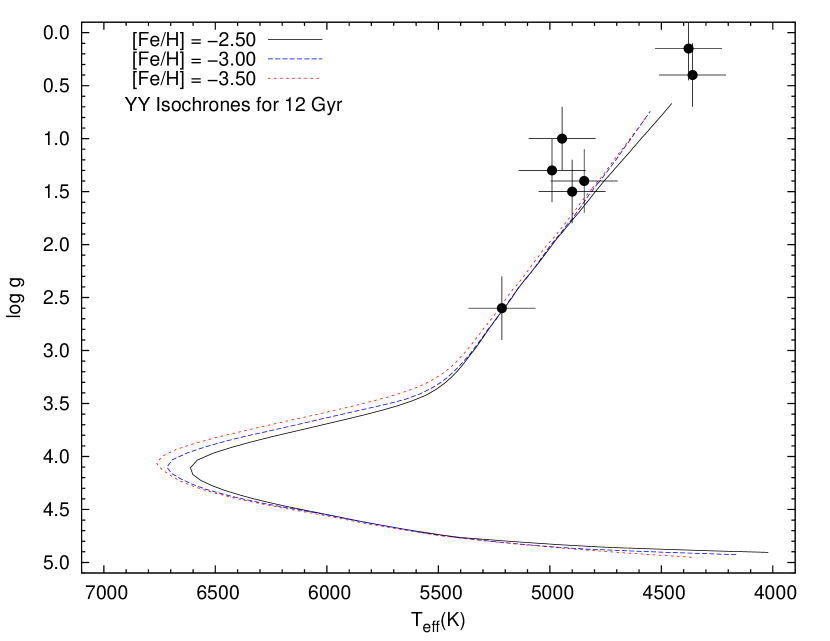
Figure 3.— H-R diagram for the program stars in this work. The parameters listed are derived from the high-resolution spectra (see Table 3). Overplotted are the Yale-Yonsei isochrones (Demarque et al., 2004) for ages of 12 Gyr and 3 different values of [Fe/H].

The final atmospheric parameters for our program stars are listed in Table 3. Note the good agreement between the [Fe/H] values derived from the medium- and high-resolution analyses. The $T_{\rm eff}$  determinations also agree within 1-$\sigma$ for all program stars. However, there remain disagreements in the log $g$ estimates, which are greater for the targets with $T_{\rm eff}$  $<$ 4400 K. These temperatures are close to the limits of the grids of medium-resolution synthetic spectra used by the n-SSPP, which is the likely source of the discrepancies. Besides that, some of the features used by the n-SSPP to determine log $g$  estimates are not present in the spectra of stars with $T_{\rm eff}$  $<$ 4400 K. Figure 3 shows the behavior of the corrected $T_{\rm eff}$  and log $g$ , compared with 12 Gyr Yale-Yonsei Isochrones (Demarque et al., 2004) for [Fe/H] = $-$3.5, $-$3.0, and $-$2.5.

4. Abundance Analysis

Table 4 lists the derived elemental abundances (or upper limits) for 20 elements estimated from the MIKE spectra. The $\sigma$ values listed in the tables are the standard error of the mean. A description of the abundance analysis results is provided below.

4.1. Techniques

Our abundance analysis makes use of one-dimensional plane-parallel model atmospheres with no overshooting (Castelli & Kurucz, 2004), computed under the assumption of local thermodynamic equilibrium (LTE). We use the 2011 version of the MOOG synthesis code (Sneden, 1973), with scattering treated with a source function that sums both absorption and scattering components, rather than treating continuous scattering as true absorption (Sobeck et al., 2011).

4.2. Abundances and Upper Limits

Elemental abundance ratios, [X/Fe], are calculated taking solar abundances from Asplund et al. (2009). Upper limits for elements for which no lines could be detected can provide useful additional information for the interpretation of the overall abundance pattern, and its possible origin. Based on the S/N ratio in the spectral region of the line, and employing the formula given in Frebel et al. (2006a), we derive 3$\sigma$ upper limits for Zn, Y and Eu. The abundance uncertainties, as well as the systematic uncertainties in the abundance estimates due to the atmospheric parameters, were treated in the same way as described in Placco et al. (2013). Table 5 shows how changes in each atmospheric parameter affect the determined abundances. Also shown is the total uncertainty for each element. In the following we present results from the abundance analysis; discussion and interpretation of these results is provided in Section 5.

4.2.1 Carbon and Nitrogen

Carbon abundances were determined from the molecular CH $G-$band feature at 4313  Å. Data for CH molecular lines were gathered from the compilation of Frebel et al. (2007), and references therein. For HE 0139$-$2826, HE 2323$-$6549, and HE 2318$-$1621, which present the largest carbon abundance ratios of our sample ([C/Fe] = $+$0.48, $+$0.72, and $+$1.04, respectively), it was possible to make a second determination using the 4322 Å region. The left panels of Figure 4 show examples of the carbon spectral synthesis for three of our program stars.

We attempted to determine nitrogen abundances from the NH band feature at 3360 Å, which is in the lowest S/N part of the observed high-resolution spectra. The line list for the NH feature was provided by Kurucz (1993), following the prescription of Aoki et al. (2006). For HE 0139$-$2826, HE 2141$-$3741, HE 2157$-$3404, HE 2318$-$1621, and HE 2323$-$6549, the molecular band could be synthesized, but the errors are between 0.2 and 0.5 dex, because data quality was low. The right panels of Figure 4 show examples of the nitrogen spectral synthesis for three of our program stars. For HE 0048$-$6408, and HE 2233$-$4724, we were only able to estimate a range of values for the nitrogen abundance ratios ([N/Fe] = $[-0.28,+0.92]$ and $[-0.48,+0.72]$, respectively).

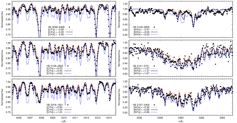
Figure 4.— left panels: example of a ch band used for carbon abundance determination. right panels: example of a nh band used for nitrogen abundance determination. the dots represent the observed spectra, the solid line is the best abundance fit, and the dotted and dashed lines are the lower and upper abundance limits, respectively, used to estimate the uncertainty.

4.2.2 From Na to Zn

For all program stars, abundances for Na, Mg, Si, K, Ca, Sc, Ti, V, Cr, Co and Ni were determined from equivalent-width analysis only (see Table 2). Aluminum abundances were determined using synthesis of the 3944 Å line, and the derived values agree with those obtained from equivalent-width measurements for both the 3944 Å and 3961 Å lines. For HE 2157$-$3404, the same agreement between synthesis and equivalent-width measurements is found for three Mn lines: 4754 Å, 4783 Å, and 4823 Å. The Mn abundances for the other program stars were determined via equivalent-width analysis. Two Si lines (3906 Å and 4103 Å) were measured in each star, and their abundances were determined via equivalent-width analysis only.

Titanium lines are found in two different ionization stages in the MIKE spectra. The agreement between the titanium abundances derived from these lines can also be used to assess the value of the surface gravity for the star. The differences between Ti I and Ti II abundances are within 0.12 dex for five of our program stars. There are larger differences for two program stars: HE 0048$-$6408 (0.29 dex) and HE 2141$-$3741 (0.25 dex). These could be related to the small number of measured lines for Ti I (5 and 3 lines, respectively). For Zn, two lines were measured: 4722 Å and 4810 Å. For HE 2141$-$3741 and HE 2323$-$6549, only upper limits on the Zn abundance could be determined.

4.2.3 Neutron-Capture Elements

Abundances for neutron-capture elements were calculated via spectral synthesis. For weak spectral features, upper limits were determined following the procedure described in Frebel et al. (2006a).

Strontium, Yttrium

The abundances of these elements are mostly determined from absorption lines in the blue spectral regions. The Sr 4077 Å and 4215 Å lines were measurable in all program stars. In the case of Y, abundances were derived from the 3774 Å line for five program stars; only an upper limit on the Y abundances was obtained for HE 2323$-$6549. No measurements or upper limits were made for HE 2318$-$1621. In addition, the 3950 Å line was used for upper-limit determinations of two program stars. The upper panels of Figure 5 show the spectral synthesis of the Sr 4077 Å for three of the program stars.

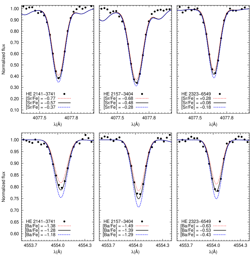
Figure 5.— Spectral synthesis of the Sr 4077 Å (upper panels) and Ba 4554 Å (lower panels) lines, for three program stars. The dots represent the observed spectra, the solid line is the best abundance fit, and the dotted and dashed line are the lower and upper abundance limits, indicating the abundance uncertainty.

Barium

Ba is mainly produced by the $s$-process in solar-system material, but it is mostly produced by the $r$-process at low metallicity (Sneden et al., 2008). It is a useful species, as it possesses lines of sufficient strength to be detected even in stars with [Fe/H] $\lesssim-3.5$. Figure 5 shows the spectral synthesis for the 4554 Å line. In addition to this feature, the 4934 Å was also used for abundance determinations for all program stars.

Europium

Eu is often taken as a reference element for the neutron-capture elements that were mainly produced by the $r$-process in solar-system material, but it can also be produced by the $s$-process in asymptotic giant branch (AGB) nucleosynthesis. We were not able to determine abundances for Eu, due to the non-detection of the spectral features. Therefore, upper limits were determined from the 4129 Å and 4205  Å lines.

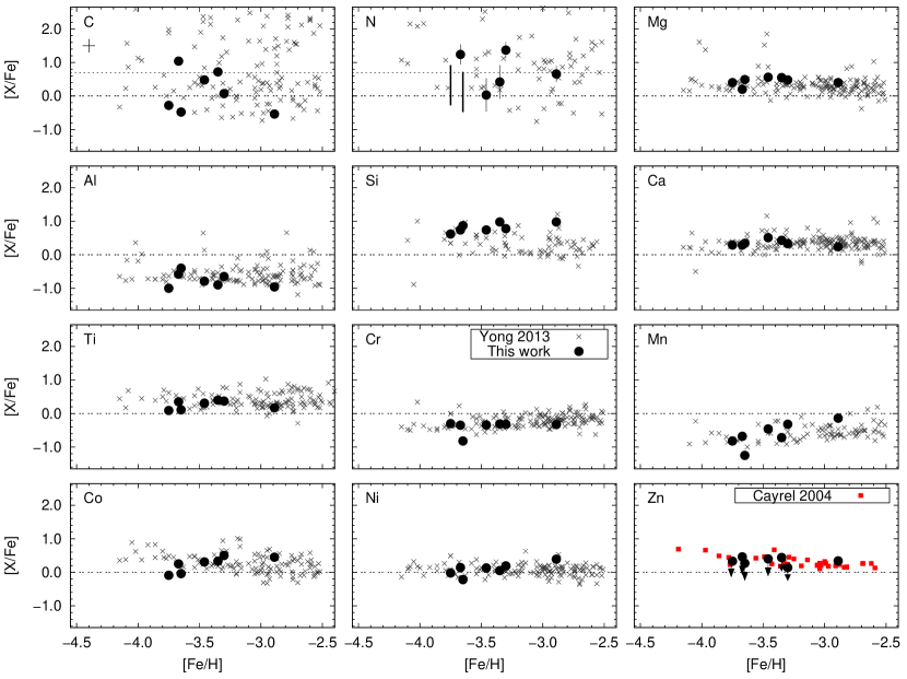
Figure 6.— Abundance ratios versus [Fe/H] for carbon, nitrogen, light elements and iron-peak elements, for stars with [Fe/H] $<-$2.5. The circles represent the stars observed in this work, while the squares are data taken from Cayrel et al. (2004), and crosses are data from Yong et al. (2013a). Arrows represent upper limits. Typical error bars are shown in the top left panel.

5. Comparison with Other Studies and Interpretations

Observation of new stars in the range of metallicity [Fe/H] $\leq-3.5$ is of importance to obtain a proper understanding of the low-metallicity tail of the Galactic MDF. The addition of HE 0048$-$6408 ([Fe/H] = $-$3.75), HE 0139-2826 ([Fe/H] =  $-$3.46), HE 2233$-$4724 ([Fe/H] = $-$3.65), and HE 2318$-$1621 ([Fe/H] = $-$3.67) to the current number of EMP stars presents new evidence that the cutoff of the MDF at [Fe/H] = $-$3.6 (Schörck et al., 2009; Li et al., 2010) may be due to selection biases. Indeed, the recent work of Yong et al. (2013b) presents 10 new stars with [Fe/H] $<-$3.5, and the tail of the low-metallicity MDF when these data are included exhibits a smooth decrease down to [Fe/H] = $-$4.1. As pointed out by these authors, these data provide a new upper limit on the MDF cutoff, and further observations in the [Fe/H] $<-$4 regime are required to address whether or not this feature is a real cutoff or simply limited by small-number statistics.

We also compared the observed chemical abundances of our program stars with data from high-resolution studies of metal-poor stars found in the literature. This was done to identify possible deviations from the general chemical abundance trends, and also to test different approaches for describing these differences, if any. Figure 6 shows the distribution of carbon, nitrogen, and other light-element and iron-peak abundances as a funtion of the metallicity, [Fe/H], compared to the stars with [Fe/H] $<-$2.5 from Cayrel et al. (2004) and Yong et al. (2013a). There are no significant differences in the abundance trends between the program stars and the objects from the literature.

5.1. CEMP Dependency on the Luminosity

As can be seen from Figure  6, C and N present a larger scatter than the remaining elements, which is believed to be due to different formation scenarios. In particular, the CEMP stars are the subject of a number of recent studies, which have attemped to determine their abundance patterns and reproduce the main features by comparison with theoretical models (e.g., Bisterzo et al., 2009; Masseron et al., 2010; Bisterzo et al., 2012, among others). HE 2318$-$1621, with [C/Fe]$\ =+$1.04, is clearly a CEMP star. Besides that, one star in the upper left-hand panel of Figure 6, HE 2323$-$6549, is right above the [C/Fe] = $+$0.7 line, indicating that it might be a CEMP star. However, this classification does not take into account evolutionary mixing effects, which can modify the initial C (and similarly, N and O) abundances of the surface of the star.

Aoki et al. (2007) suggested a CEMP classification scheme that is dependent on the luminosity of the star, in order to take into account mixing effects. Figure 7 shows the behavior of the C (upper panel) and N (lower panel) abundances as a function of the luminosity for our program stars, as well as for the data from Yong et al. (2013a). Luminosities were estimated following the prescription of Aoki et al. (2007), and assuming $M=0.8M_{\odot}$, typical of halo stars. With the exception of HE 2323$-$6549, all program stars are on the upper red-giant branch, and hence have likely suffered C-abundance depletion due to evolutionary mixing. If the luminosity criterion of Aoki et al. (2007) is adopted, six of our program stars (all with [Fe/H] $<-$3.3) could have been born as CEMP stars.

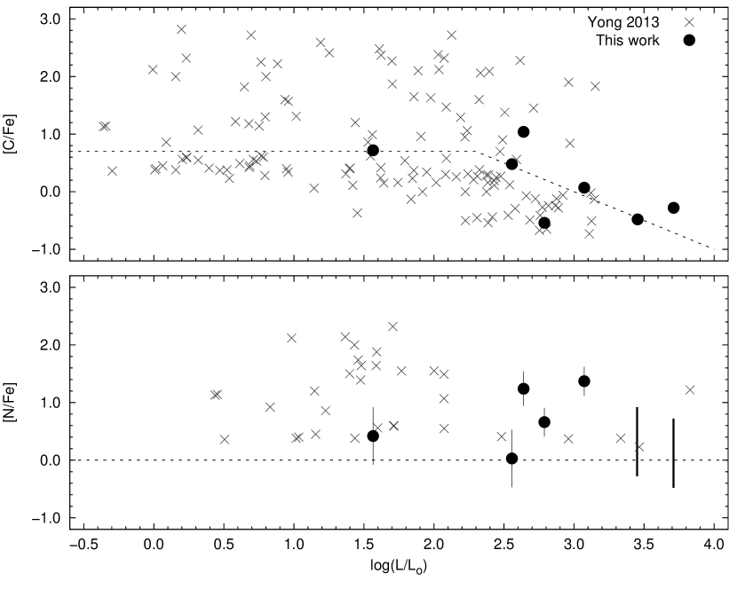
Figure 7.— Upper panel: Carbon abundances as a function of luminosity. The dashed line represents the CEMP classification of Aoki et al. (2007). Lower panel: Nitrogen abundances as a function of luminosity. The circles represent the stars observed in this work, and crosses are data from Yong et al. (2013a). The solid vertical lines for two star lines label the ranges in [N/Fe] allowed by their low-S/N spectra. The dashed line represents the solar [N/Fe] ratio.

We have assumed that the carbon-abundance depletion trend can be extrapolated beyond $\log L/L_{\odot}=3.0$. Since three of our stars have luminosities larger than $\log L/L_{\odot}=3.0$, our conclusion on the fraction of CEMP-no stars would be affected by this assumption. If the depletion trend levels off beyond $\log L/L_{\odot}=3.0$, our CEMP-no fraction would be reduced by 50%. Additional high-resolution spectroscopic studies of high-luminosity giants should help clarify this issue.

According to the Aoki et al. (2007) classification, a star with $\log L/L_{\odot}=3.5$ would be classified as CEMP if [C/Fe]$\geq-$0.5, implying a depletion of 1.2 dex of C during its evolution up the giant branch. The strong depletion of C should be accompanied by an increase in the abundance of N this star. However, evaluation of the N abundances for our program stars on the red-giant branch indicates that only HE 2141$-$3741 has a sufficiently high value ([N/Fe] $>+$1.0) to be consistent with strong C depletion. This might be an indication that, even within the CEMP classification of Aoki et al. (2007), the program stars above the CEMP line at high luminosities and with low N could have had either less C than expected ([C/Fe] $<+$0.7) during their main-sequence evolution, or have depleted more C than canonically expected. In addition, the low N abundance could also indicate lack of internal mixing in these objects, and not constrain the initial carbon abundance. This behavior must be assessed with higher S/N spectra in the NH region ($\sim$3360 Å) for the three most metal-poor stars in our sample, in order to compare their behavior with theoretical models (e.g., Stancliffe et al., 2009).

5.2. The “Forbidden Zone” and Available Fragmentation Scenarios

Chemical abundances in EMP stars can also be used to place constraints on the critical metallicity of the interstellar medium (ISM) for early star formation. Frebel et al. (2007) suggested a criteria for the formation of the first low-mass stars (“transition discriminant” – D_trans), using the [C/H] and [O/H] abundance ratios in metal-poor stars. These elements, when present in the ISM, act as efficient cooling agents, allowing gas clouds to reach temperatures and densities that enable fragmentation to a point where a low-mass star, still observable today, could be formed. Hence, there should be a threshould value (D${}_{trans}=-$3.5) below which C and O fine-structure line cooling would not be able to drive low-mass star formation (“Forbidden Zone” – see also Frebel & Norris, 2013, for more details). Figure 8 (upper panel) shows the behavior of D_trans as a function of the metallicity, [Fe/H], for our program stars and stars with [Fe/H] $<-$2.5 and [C/Fe] $<+$0.7, from Cayrel et al. (2004) and Yong et al. (2013a). The solid line shows the scaled solar D_trans value, the dashed line shows the limit of D_trans, the dotted lines show the uncertainty of the model, and the shaded area marks the Forbidden Zone.

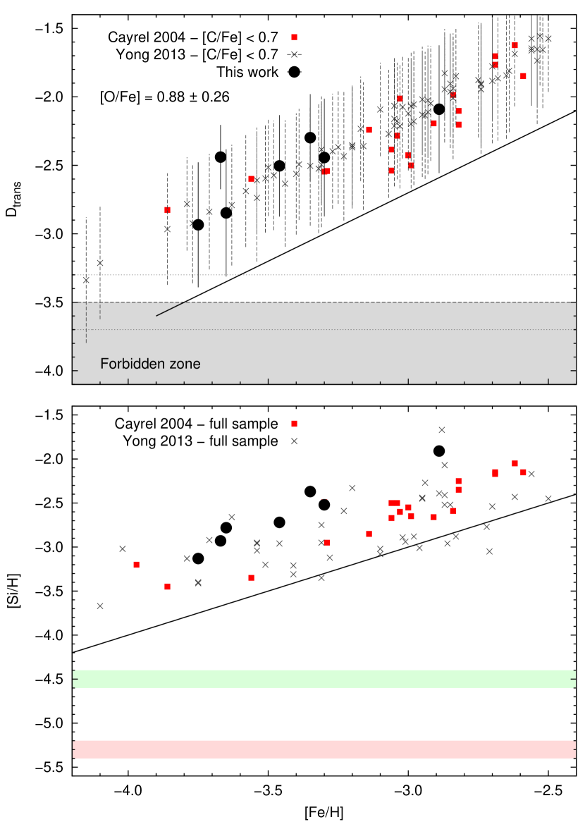
Figure 8.— Upper panel: D_trans versus [Fe/H] for the observed targets and stars from the literature with [Fe/H] $<-$2.5. The solid line shows the scaled solar abundance pattern, the dashed line shows the limit of D_trans based on the model described in Frebel et al. (2007), and the dotted lines show the uncertainty of the model. The shaded area is the Forbidden Zone, where there is insufficient C and O induced cooling for low-mass star formation. Lower panel: Silicon abundances as a function of [Fe/H]. The solid line represents [Si/Fe]=0 as a reference. The shaded areas mark the limits of the models presented in Figure 5 of Ji et al. (2013).

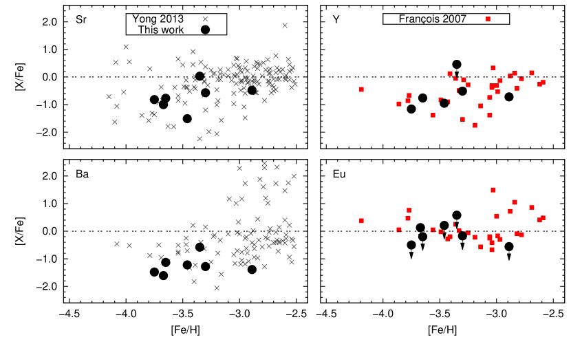
Figure 9.— Abundance ratios versus [Fe/H] for neutron-capture elements, for stars with [Fe/H] $<-$2.5. The circles represent the program stars, the squares are data taken from François et al. (2007), and the crosses are data from Yong et al. (2013a). Arrows represent upper limits.

There are no oxygen abundances available for our program stars and the Yong et al. (2013a) sample, so we estimated [O/Fe] for these targets based on the values of Cayrel et al. (2004) for stars with [C/Fe] $<+0.7$ (refer to Figure 8 of Placco et al., 2013, lower left panel). The [C/O] ratio has a linear relation with [C/Fe], with an offset of about $+0.8$ dex for the oxygen abundances. Therefore, this assumption ([O/Fe] = 0.88 $\pm$ 0.28 for [C/Fe] $<+$0.7) is a robust estimate made to calculate D_trans. The error bars on the upper panel of Figure 8 account for a 2$\sigma$ difference in [O/Fe]. It is possible to see that, for the program stars with [Fe/H] $<-$3.5, the D_trans values are above the scaled solar abundance pattern and are, within the error bars, above the Forbidden Zone, which is consistent with the cooling scenario described by Frebel et al. (2007).

Ji et al. (2013) consider an alternative fragmentation mode, the impact of thermal cooling from silicon-based dust on the formation of low-mass stars in the early universe. This channel could account for the formation of low-mass EMP stars in cases where an insufficient amount of C and O were present to induce fragmentation of the gas cloud. In fact, stars in the metallicity range [Fe/H] $<-$4 appear to exibit either high Si and low C abundances, or high C and low Si abundances. The lower panel of Figure 8 shows the behavior of the [Si/H] abundance as a function of the metallicity for the program stars and stars from the literature. The solid line represents [Si/Fe] = 0, and the shaded areas show the lower limits on the Si abundances that would allow fragmentation (see Figure 5 of Ji et al., 2013, for further details on the models). One can see that our program stars, as well as the stars from Cayrel et al. (2004) and Yong et al. (2013a), lie above the limits using both criteria, so their formation can be explained by either one of these processes. It is important to note that these stars are not sufficiently metal poor to be used as upper limits to test these models, since they were likely formed from gas enriched by multiple SNe.

Assuming the formation of EMP stars occured according to one of the criteria described above, we now examine the enrichment scenarios that would yield the required early metals prior to the formation of the stars. Figure 9 shows the distribution of selected neutron-capture element abundances as a function of the metallicity for our program stars, compared to the data from François et al. (2007) and Yong et al. (2013a), for stars with [Fe/H] $<-$2.5. All program stars appear to follow the trends presented by other studies. The Ba abundances of the stars ([Ba/Fe] $<$ 0.0), along with their C abundances (with exception of HE 2157$-$3404), suggest that these could be classified as CEMP-no stars (see Beers & Christlieb, 2005, and Figure 7 above).

While it is true that the six EMP stars presented in this work meet the CEMP criteria from Aoki et al. (2007), this is based on C abundances and estimated luminosities alone. We recognize that with such low derived C abundances, in order to be confident of their classification as CEMP stars, more accurate N abundances are needed. This would enable us to justify that substantial mixing with the products of CN-processing has indeed occurred in these stars, resulting in the transformation of C to N. Nevertheless, for completeness, below we discuss the likely formation scenarios for CEMP-no stars.

In this context, the gas clouds from which the stars were formed would have to contain C over-abundances, but lack substantial amounts of neutron-capture elements in their composition. Two models that can account for this abundance pattern are the first-generation, rapidly-evolving core-collapse SN of Nomoto et al. (2006) and the massive, rapidly rotating, MMP stars of Meynet et al. (2006). Even though both models qualitatively account for the carbon and light-element abundance patterns found in EMP stars, they predict rather different abundances of N, which could explain the increasing scatter of [N/Fe] at lower metallicities.

5.3. The [Sr/Ba] Abundance Ratios

We can also make use of abundance ratios such as [Sr/Ba] to assess the likely nucleosynthesis pathways of the progenitors of our program stars. It has been argued that elements may be formed in different astrophysical sites, since they require different neutron fluxes for their formation (Qian & Wasserburg, 2003). However, the recent study by Aoki et al. (2013) suggests that both elements are produced in the same event (e.g., SNe II), but their observed ratio depends on specific features of the progenitor, such as the collapse time of the star into a black hole. In this view, the observed [Sr/Ba] ratios could be explained by the operation of a $tr$-process (“truncated $r$-process” – see Boyd et al., 2012, for further details) at early times in the universe.

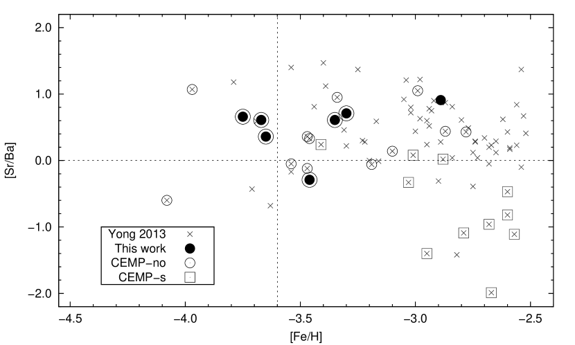
Figure 10.— [Sr/Ba] abundance ratio versus [Fe/H], for stars with [Fe/H] $<-$2.5. The filled circles represent the stars observed in this work, the filled squares are data taken from François et al. (2007), and crosses are data from Yong et al. (2013a). Open circles and squares around the symbols mark, respectively, the CEMP-no and CEMP-$s$ stars of each sample.

Figure 10 shows the [Sr/Ba] abundance ratio for the program stars, as well as data from François et al. (2007) and from Yong et al. (2013a). Also shown are the CEMP-$s$ ([C/Fe] $>+$0.7 and [Ba/Fe] $>+$1.0) and CEMP-no ([C/Fe] $>+$0.7 and [Ba/Fe] $<$ 0.0) stars identified in each sample. The presence of low [Sr/Ba] ratios at [Fe/H] $>-3.0$ is expected, since this metallicity regime is thought to reflect the onset of the $s$-process in the Galaxy (see Simmerer et al., 2004; Sivarani et al., 2004, for further details), and Ba is mainly formed by the $s$-process in solar-system material (85% according to Burris et al., 2000). Moreover, the majority of these stars are CEMP-$s$ (with [Ba/Fe] $>+$1.0), whose abundance patterns are a direct evidence of mass transfer episodes from a low-mass AGB star in a binary system (see Placco et al., 2013, for further details).

In the [Fe/H] $<-3.0$ regime, the formation of Sr and Ba is likely dominated by the $r$-process (or alternatively by the $tr$-process, as mentioned above, or else by an $s$-process associated with the explosions of massive stars; see Cescutti et al., 2013). There appears to exist increasing scatter for [Sr/Ba] ratios with decreasing metallicity, which is consistent with the behavior of the data analyzed by Aoki et al. (2013). However, a number of stars exhibit [Sr/Ba] ratios that are not entirely consistent with the cutoff at [Sr/Ba] $>$ 0.0 suggested by Aoki et al. (2013).

6. Conclusions

In this work we analyzed seven newly discovered VMP/EMP stars, originally selected from the low-resolution HES plates, and followed up with medium-resolution, then high-resolution spectroscopy. According to our analysis of the high-resolution spectra, six of them exhibit [Fe/H] $<-$3.0, and four have [Fe/H] $\leq-$3.5.

We have analyzed selected light and neutron-capture elements for the program stars; there are no significant abundance differences when compared with results from the literature. Six of our targets are consistent with the CEMP-no classification of Aoki et al. (2007), and exhibit enhancements in C (corrected for evolutionary mixing) and a lack of neutron-capture elements ([Ba/Fe] $<$ 0.0). However, more accurate N abundances are needed in order to confirm this. The abundances in the sample are also consistent with C-normal EMP stars from the literature, and can also be used to study the yields of the early stellar generations to form in the Galaxy.

It is worth emphasizing that the [Fe/H] $<-$3.5 metallicity regime is of particular importance in determining the true shape of the MDF, and further observations of EMP stars can help understand whether the observed MDF tail at [Fe/H] = $-$4.1 is real or a result of an incomplete inventory of low-metallicity stars.

Table 1Observational Data for the Observed Candidates

	HE 0048$-$6408	HE 0139$-$2826	HE 2141$-$3741	HE 2157$-$3404	HE 2233$-$4724	HE 2318$-$1621	HE 2323$-$6549
$\alpha$ (J2000)	00:50:45.3	01:41:36.8	21:44:51.1	22:00:17.6	22:35:59.2	23:21:21.5	23:26:14.5
$\delta$ (J2000)	$-$63:51:50.0	$-$28:11:03.0	$-$37:27:55.0	$-$33:50:04.0	$-$47:08:36.0	$-$16:05:06.0	$-$65:33:06.0
V (mag)	12.9	13.7	13.4	13.2	14.8	13.1	14.3
($J-K$)0	0.63	0.53	0.51	0.53	0.64	0.51	0.50
KP ( Å)	4.1	4.0	2.8	4.9	6.6	3.7	4.5
Medium Resolution
Date	2011 10 17	2011 10 17	2011 08 03	2011 08 03	2011 10 17	2011 10 17	2011 08 03
UT	04:27:26	06:09:16	03:33:00	04:11:00	01:16:05	02:57:46	08:29:00
Exptime (s)	120	180	1400	1000	720	120	1800
Telescope	ESO/NTT	ESO/NTT	SOAR	SOAR	ESO/NTT	ESO/NTT	SOAR
High Resolution – Magellan/MIKE
Date	2012 09 09	2012 09 09	2011 11 03	2011 11 03	2012 09 09	2013 10 26	2011 11 03
UT	04:03:29	06:33:57	00:00:35	01:48:45	04:46:49	02:43:57	05:14:32
Exptime (s)	2400	2100	1400	900	3600	7200	3400
vr(km/s)	$-$33.1	$-$253.0	$-$170.5	$-$11.6	$-$166.6	$-$4.1	23.6

Table 2 Equivalent Width Measurements

				HE0048$-$6408		HE0139$-$2826		HE2141$-$3741		HE2157$-$3404		HE2233$-$4724		HE2318$-$1621		HE2323$-$6549
Ion	$\lambda$	$\chi$	$\log\,gf$	$W$	$\log\epsilon$	$W$	$\log\epsilon$	$W$	$\log\epsilon$	$W$	$\log\epsilon$	$W$	$\log\epsilon$	$W$	$\log\epsilon$	$W$	$\log\epsilon$
	Å	eV		mÅ		mÅ		mÅ		mÅ		mÅ		mÅ		mÅ
C CH	4313.00	$\cdots$	$\cdots$	syn	4.4	syn	5.4	syn	5.2	syn	5.0	syn	4.3	syn	5.30	syn	5.8
C CH	4322.00	$\cdots$	$\cdots$	$\cdots$	$\cdots$	syn	5.5	$\cdots$	$\cdots$	$\cdots$	$\cdots$	$\cdots$	$\cdots$	syn	5.30	syn	5.8
N NH	3360.00	$\cdots$	$\cdots$	$\cdots$	$\cdots$	syn	4.4	syn	5.9	syn	5.6	$\cdots$	$\cdots$	syn	5.40	syn	4.9
Na I	5889.95	0.00	0.11	134.7	2.6	121.4	3.3	127.6	3.3	165.9	4.0	192.8	3.3	0.1	0.00	126.6	3.6
Na I	5895.92	0.00	$-$0.19	102.7	2.5	100.1	3.2	98.9	3.1	131.0	3.7	167.1	3.2	108.7	3.28	94.0	3.3
Mg I	3829.36	2.71	$-$0.21	$\cdots$	$\cdots$	130.0	4.8	128.7	4.7	$\cdots$	$\cdots$	$\cdots$	$\cdots$	96.9	3.94	125.7	4.7
Mg I	3832.30	2.71	0.27	$\cdots$	$\cdots$	150.1	4.6	$\cdots$	$\cdots$	$\cdots$	$\cdots$	$\cdots$	$\cdots$	$\cdots$	$\cdots$	$\cdots$	$\cdots$
Mg I	3838.29	2.72	0.49	$\cdots$	$\cdots$	169.5	4.6	$\cdots$	$\cdots$	$\cdots$	$\cdots$	$\cdots$	$\cdots$	130.6	4.02	$\cdots$	$\cdots$
Mg I	4057.51	4.35	$-$0.89	$\cdots$	$\cdots$	$\cdots$	$\cdots$	$\cdots$	$\cdots$	29.0	5.2	$\cdots$	$\cdots$	$\cdots$	$\cdots$	$\cdots$	$\cdots$
Mg I	4167.27	4.35	$-$0.71	12.2	4.2	18.7	4.7	$\cdots$	$\cdots$	34.2	5.1	$\cdots$	$\cdots$	11.5	4.41	18.7	4.8
Mg I	4702.99	4.33	$-$0.38	23.2	4.2	38.1	4.7	29.4	4.6	59.0	5.1	$\cdots$	$\cdots$	11.9	4.05	26.8	4.7
Mg I	5172.68	2.71	$-$0.45	151.7	4.2	$\cdots$	$\cdots$	147.0	4.9	$\cdots$	$\cdots$	180.6	4.5	104.4	4.08	142.1	4.9
Mg I	5183.60	2.72	$-$0.24	168.8	4.3	154.2	4.8	156.0	4.9	$\cdots$	$\cdots$	191.6	4.4	121.1	4.21	156.3	4.9
Mg I	5528.40	4.34	$-$0.50	25.0	4.3	30.9	4.7	33.9	4.8	52.6	5.1	30.5	4.4	10.5	4.10	29.7	4.8
Al I	3944.01	0.00	$-$0.64	$\cdots$	$\cdots$	$\cdots$	$\cdots$	$\cdots$	$\cdots$	102.5	3.0	$\cdots$	$\cdots$	$\cdots$	$\cdots$	84.7	2.9
Al I	3944.01	0.00	$-$0.64	syn	1.7	syn	2.2	syn	2.5	syn	2.6	syn	2.4	syn	2.2	syn	2.2
Al I	3961.52	0.01	$-$0.34	98.8	1.9	69.8	2.0	$\cdots$	$\cdots$	109.8	2.9	133.1	2.4	85.4	2.30	63.4	2.2
Si I	3905.52	1.91	$-$1.09	160.8	4.4	$\cdots$	$\cdots$	145.6	5.0	$\cdots$	$\cdots$	195.5	4.7	127.3	4.58	139.4	5.0
Si I	4102.94	1.91	$-$3.14	53.4	4.3	41.9	4.8	$\cdots$	$\cdots$	83.6	5.6	87.5	4.8	$\cdots$	$\cdots$	51.8	5.3
K I	7664.90	0.00	0.14	$\cdots$	$\cdots$	28.7	2.5	$\cdots$	$\cdots$	$\cdots$	$\cdots$	36.1	2.1	$\cdots$	$\cdots$	$\cdots$	$\cdots$
K I	7698.96	0.00	$-$0.17	9.9	1.8	9.8	2.2	$\cdots$	$\cdots$	$\cdots$	$\cdots$	$\cdots$	$\cdots$	$\cdots$	$\cdots$	$\cdots$	$\cdots$
Ca I	4226.73	0.00	0.24	$\cdots$	$\cdots$	136.3	3.3	145.0	3.4	$\cdots$	$\cdots$	$\cdots$	$\cdots$	117.4	2.80	129.0	3.3
Ca I	4283.01	1.89	$-$0.22	16.0	2.8	23.8	3.4	21.4	3.3	35.9	3.7	24.8	2.9	15.6	3.08	18.6	3.4
Ca I	4318.65	1.89	$-$0.21	16.1	2.7	25.8	3.4	20.1	3.3	36.1	3.7	25.0	2.9	12.4	2.95	19.7	3.4
Ca I	4425.44	1.88	$-$0.36	12.1	2.7	16.9	3.3	$\cdots$	$\cdots$	27.3	3.6	21.2	3.0	9.1	2.93	17.4	3.5
Ca I	4434.96	1.89	$-$0.01	$\cdots$	$\cdots$	40.3	3.5	34.8	3.4	$\cdots$	$\cdots$	41.4	3.0	16.8	2.89	26.9	3.4
Ca I	4435.69	1.89	$-$0.52	$\cdots$	$\cdots$	15.9	3.4	$\cdots$	$\cdots$	21.0	3.6	$\cdots$	$\cdots$	10.5	3.17	$\cdots$	$\cdots$
Ca I	4454.78	1.90	0.26	$\cdots$	$\cdots$	43.1	3.3	44.0	3.3	59.7	3.6	$\cdots$	$\cdots$	24.3	2.84	38.5	3.4
Ca I	4455.89	1.90	$-$0.53	11.2	2.9	11.9	3.3	$\cdots$	$\cdots$	22.4	3.7	20.2	3.1	$\cdots$	$\cdots$	11.5	3.5
Ca I	5262.24	2.52	$-$0.47	$\cdots$	$\cdots$	5.7	3.5	$\cdots$	$\cdots$	$\cdots$	$\cdots$	$\cdots$	$\cdots$	$\cdots$	$\cdots$	$\cdots$	$\cdots$
Ca I	5588.76	2.52	0.21	$\cdots$	$\cdots$	20.9	3.5	$\cdots$	$\cdots$	30.0	3.8	17.7	3.1	8.4	3.00	11.6	3.4
Ca I	5594.47	2.52	0.10	9.7	2.9	16.6	3.5	12.2	3.4	22.5	3.7	$\cdots$	$\cdots$	$\cdots$	$\cdots$	12.1	3.5
Ca I	5598.49	2.52	$-$0.09	$\cdots$	$\cdots$	11.5	3.5	$\cdots$	$\cdots$	$\cdots$	$\cdots$	$\cdots$	$\cdots$	$\cdots$	$\cdots$	$\cdots$	$\cdots$
Ca I	5857.45	2.93	0.23	$\cdots$	$\cdots$	$\cdots$	$\cdots$	5.7	3.3	$\cdots$	$\cdots$	$\cdots$	$\cdots$	$\cdots$	$\cdots$	$\cdots$	$\cdots$
Ca I	6102.72	1.88	$-$0.79	9.9	3.0	$\cdots$	$\cdots$	$\cdots$	$\cdots$	18.5	3.8	$\cdots$	$\cdots$	4.4	2.95	6.5	3.4
Ca I	6122.22	1.89	$-$0.32	24.1	3.0	25.9	3.4	25.7	3.5	38.8	3.7	30.9	3.1	12.7	2.98	20.4	3.5
Ca I	6162.17	1.90	$-$0.09	31.9	2.9	33.4	3.4	35.6	3.4	51.4	3.7	49.4	3.1	16.2	2.89	27.1	3.4
Ca I	6439.07	2.52	0.47	20.2	2.9	24.0	3.3	24.7	3.3	39.4	3.6	26.0	3.0	15.6	3.01	$\cdots$	$\cdots$
Ca I	6449.81	2.52	$-$0.50	$\cdots$	$\cdots$	5.1	3.5	$\cdots$	$\cdots$	$\cdots$	$\cdots$	$\cdots$	$\cdots$	$\cdots$	$\cdots$	$\cdots$	$\cdots$
Sc II	4246.82	0.32	0.24	107.4	$-$0.8	85.3	$-$0.2	105.7	$\cdots$	114.1	0.3	$\cdots$	$\cdots$	63.3	$-$0.77	59.5	$-$0.2
Sc II	4314.08	0.62	$-$0.10	$\cdots$	$\cdots$	53.3	$-$0.2	70.5	$-$0.1	86.1	0.3	91.2	$-$0.4	31.0	$-$0.69	25.3	$-$0.2
Sc II	4325.00	0.59	$-$0.44	47.3	$-$0.8	40.2	$-$0.1	51.6	$-$0.1	66.0	0.3	62.7	$-$0.6	16.0	$-$0.76	$\cdots$	$\cdots$
Sc II	4400.39	0.61	$-$0.54	40.3	$-$0.8	34.4	$-$0.1	42.3	$-$0.1	58.8	0.3	60.9	$-$0.5	11.1	$-$0.82	12.1	$-$0.2
Sc II	4415.54	0.59	$-$0.67	35.0	$-$0.8	23.2	$-$0.3	39.7	$-$0.1	54.3	0.3	51.5	$-$0.5	8.8	$-$0.83	$\cdots$	$\cdots$
Sc II	5031.01	1.36	$-$0.40	11.6	$-$0.7	$\cdots$	$\cdots$	15.4	$-$0.0	18.1	0.2	$\cdots$	$\cdots$	$\cdots$	$\cdots$	$\cdots$	$\cdots$
Sc II	5526.78	1.77	0.02	$\cdots$	$\cdots$	$\cdots$	$\cdots$	$\cdots$	$\cdots$	22.7	0.3	22.3	$-$0.2	$\cdots$	$\cdots$	$\cdots$	$\cdots$
Sc II	5657.91	1.51	$-$0.60	$\cdots$	$\cdots$	$\cdots$	$\cdots$	$\cdots$	$\cdots$	13.5	0.3	$\cdots$	$\cdots$	$\cdots$	$\cdots$	$\cdots$	$\cdots$
Ti I	3989.76	0.02	$-$0.06	$\cdots$	$\cdots$	$\cdots$	$\cdots$	$\cdots$	$\cdots$	40.3	2.1	$\cdots$	$\cdots$	18.3	1.43	$\cdots$	$\cdots$
Ti I	3998.64	0.05	0.01	$\cdots$	$\cdots$	28.8	1.7	$\cdots$	$\cdots$	46.2	2.2	$\cdots$	$\cdots$	19.7	1.43	22.0	1.9
Ti I	4008.93	0.02	$-$1.02	6.5	1.2	$\cdots$	$\cdots$	$\cdots$	$\cdots$	$\cdots$	$\cdots$	$\cdots$	$\cdots$	$\cdots$	$\cdots$	$\cdots$	$\cdots$
Ti I	4533.25	0.85	0.53	18.1	1.2	19.0	1.8	$\cdots$	$\cdots$	31.1	2.2	24.3	1.3	11.5	1.51	15.2	2.0
Ti I	4534.78	0.84	0.34	12.0	1.2	10.3	1.7	17.4	2.1	24.9	2.3	$\cdots$	$\cdots$	7.5	1.49	11.4	2.1
Ti I	4535.57	0.83	0.12	10.0	1.3	$\cdots$	$\cdots$	$\cdots$	$\cdots$	16.3	2.3	17.0	1.5	$\cdots$	$\cdots$	$\cdots$	$\cdots$
Ti I	4681.91	0.05	$-$1.01	5.4	1.2	$\cdots$	$\cdots$	$\cdots$	$\cdots$	$\cdots$	$\cdots$	$\cdots$	$\cdots$	$\cdots$	$\cdots$	$\cdots$	$\cdots$
Ti I	4981.73	0.84	0.56	$\cdots$	$\cdots$	19.0	1.8	23.8	2.0	33.6	2.2	27.7	1.3	12.0	1.46	12.3	1.9
Ti I	4991.07	0.84	0.44	18.3	1.3	20.5	1.9	$\cdots$	$\cdots$	31.7	2.3	27.6	1.4	$\cdots$	$\cdots$	$\cdots$	$\cdots$
Ti I	4999.50	0.83	0.31	14.3	1.3	12.2	1.8	17.0	2.0	21.4	2.2	22.2	1.4	$\cdots$	$\cdots$	12.4	2.1
Ti I	5007.21	0.82	0.17	14.0	1.4	$\cdots$	$\cdots$	$\cdots$	$\cdots$	20.4	2.3	$\cdots$	$\cdots$	8.8	1.68	$\cdots$	$\cdots$
Ti I	5014.28	0.81	0.11	10.0	1.3	11.3	1.9	$\cdots$	$\cdots$	$\cdots$	$\cdots$	$\cdots$	$\cdots$	$\cdots$	$\cdots$	$\cdots$	$\cdots$
Ti I	5192.97	0.02	$-$0.95	11.0	1.4	$\cdots$	$\cdots$	$\cdots$	$\cdots$	$\cdots$	$\cdots$	$\cdots$	$\cdots$	$\cdots$	$\cdots$	$\cdots$	$\cdots$
Ti I	5210.39	0.05	$-$0.83	13.8	1.4	$\cdots$	$\cdots$	$\cdots$	$\cdots$	14.4	2.2	$\cdots$	$\cdots$	$\cdots$	$\cdots$	$\cdots$	$\cdots$
Ti II	3489.74	0.14	$-$1.98	$\cdots$	$\cdots$	53.9	1.7	$\cdots$	$\cdots$	$\cdots$	$\cdots$	$\cdots$	$\cdots$	43.4	1.43	36.9	2.0
Ti II	3491.05	0.11	$-$1.15	$\cdots$	$\cdots$	85.5	1.8	$\cdots$	$\cdots$	$\cdots$	$\cdots$	$\cdots$	$\cdots$	76.5	1.43	77.8	2.2
Ti II	3759.29	0.61	0.28	$\cdots$	$\cdots$	124.1	1.8	$\cdots$	$\cdots$	163.8	2.3	$\cdots$	$\cdots$	109.1	1.33	108.2	2.0
Ti II	3761.32	0.57	0.18	$\cdots$	$\cdots$	119.5	1.8	$\cdots$	$\cdots$	165.7	2.4	$\cdots$	$\cdots$	105.5	1.28	103.0	1.9
Ti II	3813.39	0.61	$-$2.02	$\cdots$	$\cdots$	$\cdots$	$\cdots$	45.1	1.9	66.1	2.4	$\cdots$	$\cdots$	20.4	1.41	24.6	2.1
Ti II	3882.29	1.12	$-$1.71	$\cdots$	$\cdots$	21.4	1.8	$\cdots$	$\cdots$	39.7	2.1	$\cdots$	$\cdots$	$\cdots$	$\cdots$	$\cdots$	$\cdots$
Ti II	4012.40	0.57	$-$1.75	73.7	1.3	52.4	1.8	$\cdots$	$\cdots$	77.3	2.2	84.9	1.5	28.4	1.27	28.8	1.9
Ti II	4025.12	0.61	$-$1.98	50.1	1.2	26.6	1.6	$\cdots$	$\cdots$	54.2	2.1	64.5	1.4	16.7	1.24	21.1	2.0
Ti II	4028.34	1.89	$-$0.96	$\cdots$	$\cdots$	13.4	1.6	$\cdots$	$\cdots$	31.8	2.1	$\cdots$	$\cdots$	$\cdots$	$\cdots$	$\cdots$	$\cdots$
Ti II	4053.83	1.89	$-$1.21	12.4	1.2	12.3	1.9	$\cdots$	$\cdots$	23.8	2.2	19.0	1.5	6.6	1.50	$\cdots$	$\cdots$
Ti II	4161.53	1.08	$-$2.16	16.7	1.3	$\cdots$	$\cdots$	$\cdots$	$\cdots$	31.1	2.4	26.9	1.6	$\cdots$	$\cdots$	$\cdots$	$\cdots$
Ti II	4163.63	2.59	$-$0.40	9.6	1.1	9.8	1.7	$\cdots$	$\cdots$	33.2	2.3	16.2	1.5	$\cdots$	$\cdots$	$\cdots$	$\cdots$
Ti II	4184.31	1.08	$-$2.51	$\cdots$	$\cdots$	$\cdots$	$\cdots$	$\cdots$	$\cdots$	$\cdots$	$\cdots$	14.8	1.6	$\cdots$	$\cdots$	$\cdots$	$\cdots$
Ti II	4290.22	1.16	$-$0.93	64.8	1.1	61.1	1.8	69.2	1.8	87.5	2.2	85.0	1.4	38.4	1.31	41.7	2.0
Ti II	4300.05	1.18	$-$0.49	$\cdots$	$\cdots$	$\cdots$	$\cdots$	83.5	1.6	97.6	2.0	$\cdots$	$\cdots$	53.7	1.18	57.9	1.9
Ti II	4330.72	1.18	$-$2.06	15.4	1.3	$\cdots$	$\cdots$	$\cdots$	$\cdots$	22.2	2.2	21.4	1.5	$\cdots$	$\cdots$	$\cdots$	$\cdots$
Ti II	4337.91	1.08	$-$0.96	75.6	1.1	56.1	1.6	82.9	2.0	95.9	2.3	87.1	1.3	$\cdots$	$\cdots$	$\cdots$	$\cdots$
Ti II	4394.06	1.22	$-$1.78	20.9	1.2	17.1	1.8	20.6	1.8	35.0	2.2	39.6	1.6	5.6	1.19	$\cdots$	$\cdots$
Ti II	4395.03	1.08	$-$0.54	96.5	1.1	82.7	1.8	95.8	1.8	104.9	2.1	115.3	1.4	56.3	1.15	61.3	1.9
Ti II	4395.84	1.24	$-$1.93	15.2	1.2	8.3	1.6	18.0	1.9	25.3	2.2	24.3	1.5	$\cdots$	$\cdots$	$\cdots$	$\cdots$
Ti II	4399.77	1.24	$-$1.19	46.0	1.1	38.8	1.7	44.7	1.7	68.0	2.2	68.9	1.5	18.8	1.22	25.7	2.0
Ti II	4417.71	1.17	$-$1.19	57.3	1.2	40.3	1.7	57.1	1.8	74.2	2.2	73.5	1.5	21.1	1.20	27.6	1.9
Ti II	4418.33	1.24	$-$1.97	16.1	1.3	$\cdots$	$\cdots$	13.4	1.8	26.2	2.2	26.1	1.6	6.2	1.45	$\cdots$	$\cdots$
Ti II	4441.73	1.18	$-$2.41	$\cdots$	$\cdots$	$\cdots$	$\cdots$	$\cdots$	$\cdots$	14.9	2.3	$\cdots$	$\cdots$	$\cdots$	$\cdots$	$\cdots$	$\cdots$
Ti II	4443.80	1.08	$-$0.72	85.9	1.1	68.1	1.6	83.0	1.7	96.6	2.1	103.7	1.3	52.7	1.25	53.7	1.9
Ti II	4444.55	1.12	$-$2.24	$\cdots$	$\cdots$	$\cdots$	$\cdots$	12.7	1.9	22.7	2.3	23.3	1.6	$\cdots$	$\cdots$	$\cdots$	$\cdots$
Ti II	4450.48	1.08	$-$1.52	48.7	1.3	35.0	1.8	42.3	1.8	57.3	2.1	65.9	1.6	20.4	1.40	18.9	1.9
Ti II	4464.45	1.16	$-$1.81	27.3	1.3	16.3	1.7	24.4	1.8	37.9	2.2	42.8	1.6	12.9	1.54	8.8	1.9
Ti II	4468.52	1.13	$-$0.60	87.2	1.0	71.5	1.6	$\cdots$	$\cdots$	99.6	2.1	106.9	1.3	50.7	1.15	55.1	1.8
Ti II	4470.85	1.17	$-$2.02	10.7	1.0	11.2	1.8	$\cdots$	$\cdots$	23.7	2.1	29.9	1.6	$\cdots$	$\cdots$	$\cdots$	$\cdots$
Ti II	4501.27	1.12	$-$0.77	79.6	1.1	67.2	1.7	85.5	1.8	100.4	2.2	104.0	1.4	45.2	1.21	52.1	1.9
Ti II	4533.96	1.24	$-$0.53	83.8	1.0	66.2	1.6	84.0	1.7	99.8	2.1	$\cdots$	$\cdots$	48.5	1.17	53.5	1.9
Ti II	4563.77	1.22	$-$0.96	$\cdots$	$\cdots$	57.9	1.8	73.0	1.9	89.4	2.3	90.6	1.5	43.1	1.47	47.0	2.1
Ti II	4571.97	1.57	$-$0.32	70.5	1.0	56.3	1.5	74.0	1.7	88.9	2.1	$\cdots$	$\cdots$	44.0	1.26	47.5	1.9
Ti II	4589.91	1.24	$-$1.79	$\cdots$	$\cdots$	19.2	1.9	28.1	1.9	42.9	2.3	45.7	1.7	$\cdots$	$\cdots$	$\cdots$	$\cdots$
Ti II	4657.20	1.24	$-$2.24	$\cdots$	$\cdots$	$\cdots$	$\cdots$	$\cdots$	$\cdots$	$\cdots$	$\cdots$	15.5	1.6	$\cdots$	$\cdots$	$\cdots$	$\cdots$
Ti II	4708.66	1.24	$-$2.34	$\cdots$	$\cdots$	$\cdots$	$\cdots$	$\cdots$	$\cdots$	$\cdots$	$\cdots$	16.4	1.7	$\cdots$	$\cdots$	$\cdots$	$\cdots$
Ti II	4779.98	2.05	$-$1.37	$\cdots$	$\cdots$	5.3	1.7	$\cdots$	$\cdots$	14.7	2.2	11.8	1.6	$\cdots$	$\cdots$	$\cdots$	$\cdots$
Ti II	4805.09	2.06	$-$1.10	$\cdots$	$\cdots$	10.4	1.8	14.8	1.8	25.6	2.2	20.4	1.6	$\cdots$	$\cdots$	$\cdots$	$\cdots$
Ti II	5129.16	1.89	$-$1.24	$\cdots$	$\cdots$	$\cdots$	$\cdots$	$\cdots$	$\cdots$	21.7	2.1	$\cdots$	$\cdots$	$\cdots$	$\cdots$	$\cdots$	$\cdots$
Ti II	5185.90	1.89	$-$1.49	$\cdots$	$\cdots$	$\cdots$	$\cdots$	$\cdots$	$\cdots$	16.5	2.2	$\cdots$	$\cdots$	3.3	1.39	$\cdots$	$\cdots$
Ti II	5188.69	1.58	$-$1.05	36.3	1.2	$\cdots$	$\cdots$	41.4	1.8	59.3	2.2	42.6	1.4	11.7	1.18	$\cdots$	$\cdots$
Ti II	5226.54	1.57	$-$1.26	$\cdots$	$\cdots$	17.9	1.6	29.4	1.8	44.8	2.2	52.5	1.7	$\cdots$	$\cdots$	13.7	2.0
Ti II	5336.79	1.58	$-$1.59	17.0	1.3	$\cdots$	$\cdots$	14.0	1.7	26.0	2.2	$\cdots$	$\cdots$	$\cdots$	$\cdots$	$\cdots$	$\cdots$
Ti II	5381.02	1.57	$-$1.92	5.8	1.1	$\cdots$	$\cdots$	$\cdots$	$\cdots$	17.9	2.3	17.5	1.7	$\cdots$	$\cdots$	$\cdots$	$\cdots$
V I	5195.40	2.28	$-$0.12	3.8	2.9	$\cdots$	$\cdots$	$\cdots$	$\cdots$	$\cdots$	$\cdots$	$\cdots$	$\cdots$	$\cdots$	$\cdots$	$\cdots$	$\cdots$
V II	4005.71	1.82	$-$0.52	$\cdots$	$\cdots$	$\cdots$	$\cdots$	$\cdots$	$\cdots$	$\cdots$	$\cdots$	$\cdots$	$\cdots$	$\cdots$	$\cdots$	$\cdots$	$\cdots$
Cr I	3578.68	0.00	0.42	$\cdots$	$\cdots$	$\cdots$	$\cdots$	78.8	1.8	$\cdots$	$\cdots$	$\cdots$	$\cdots$	68.9	1.44	$\cdots$	$\cdots$
Cr I	4254.33	0.00	$-$0.11	$\cdots$	$\cdots$	$\cdots$	$\cdots$	79.4	2.0	95.5	2.4	$\cdots$	$\cdots$	55.3	1.40	57.0	1.9
Cr I	4274.80	0.00	$-$0.22	$\cdots$	$\cdots$	62.7	1.7	77.3	2.0	89.3	2.3	87.1	1.2	54.1	1.48	55.0	2.0
Cr I	4289.72	0.00	$-$0.37	$\cdots$	$\cdots$	56.9	1.8	67.2	2.0	83.3	2.4	75.6	1.2	45.4	1.46	48.4	2.0
Cr I	4646.15	1.03	$-$0.74	9.8	1.6	$\cdots$	$\cdots$	$\cdots$	$\cdots$	15.1	2.5	$\cdots$	$\cdots$	5.7	1.84	$\cdots$	$\cdots$
Cr I	4652.16	1.00	$-$1.03	5.5	1.6	$\cdots$	$\cdots$	$\cdots$	$\cdots$	$\cdots$	$\cdots$	$\cdots$	$\cdots$	$\cdots$	$\cdots$	$\cdots$	$\cdots$
Cr I	5206.04	0.94	0.02	48.8	1.6	34.0	1.9	43.1	2.2	59.3	2.5	$\cdots$	$\cdots$	27.4	1.74	21.9	2.0
Cr I	5208.42	0.94	0.16	57.6	1.6	41.9	1.9	47.7	2.1	$\cdots$	$\cdots$	$\cdots$	$\cdots$	34.7	1.75	33.4	2.1
Cr I	5409.77	1.03	$-$0.67	11.2	1.6	$\cdots$	$\cdots$	$\cdots$	$\cdots$	18.2	2.5	$\cdots$	$\cdots$	$\cdots$	$\cdots$	$\cdots$	$\cdots$
Cr II	3408.74	2.48	$-$0.42	37.0	1.0	$\cdots$	$\cdots$	$\cdots$	$\cdots$	$\cdots$	$\cdots$	$\cdots$	$\cdots$	40.6	1.68	$\cdots$	$\cdots$
Mn I	4030.75	0.00	$-$0.48	89.5	0.9	75.4	1.7	86.8	1.9	$\cdots$	$\cdots$	81.3	0.6	57.1	1.11	43.5	1.3
Mn I	4033.06	0.00	$-$0.62	79.4	0.8	60.5	1.4	76.8	1.8	100.3	2.4	76.2	0.6	47.4	1.05	35.3	1.3
Mn I	4034.48	0.00	$-$0.81	67.2	0.8	53.9	1.5	68.1	1.8	89.4	2.3	46.6	0.4	37.9	1.06	31.2	1.4
Mn I	4041.36	2.11	0.28	$\cdots$	$\cdots$	$\cdots$	$\cdots$	$\cdots$	$\cdots$	29.0	2.4	$\cdots$	$\cdots$	$\cdots$	$\cdots$	$\cdots$	$\cdots$
Mn I	4754.05	2.28	$-$0.09	$\cdots$	$\cdots$	$\cdots$	$\cdots$	$\cdots$	$\cdots$	11.6	2.4	$\cdots$	$\cdots$	$\cdots$	$\cdots$	$\cdots$	$\cdots$
Mn I	4754.05	2.28	$-$0.09	$\cdots$	$\cdots$	$\cdots$	$\cdots$	$\cdots$	$\cdots$	syn	2.4	$\cdots$	$\cdots$	$\cdots$	$\cdots$	$\cdots$	$\cdots$
Mn I	4783.43	2.30	0.04	$\cdots$	$\cdots$	$\cdots$	$\cdots$	$\cdots$	$\cdots$	16.1	2.5	$\cdots$	$\cdots$	$\cdots$	$\cdots$	$\cdots$	$\cdots$
Mn I	4783.43	2.30	0.04	$\cdots$	$\cdots$	$\cdots$	$\cdots$	$\cdots$	$\cdots$	syn	2.4	$\cdots$	$\cdots$	$\cdots$	$\cdots$	$\cdots$	$\cdots$
Mn I	4823.53	2.32	0.14	$\cdots$	$\cdots$	$\cdots$	$\cdots$	$\cdots$	$\cdots$	18.7	2.5	$\cdots$	$\cdots$	$\cdots$	$\cdots$	$\cdots$	$\cdots$
Mn I	4823.53	2.32	0.14	$\cdots$	$\cdots$	$\cdots$	$\cdots$	$\cdots$	$\cdots$	syn	2.4	$\cdots$	$\cdots$	$\cdots$	$\cdots$	$\cdots$	$\cdots$
Fe I	3565.38	0.96	$-$0.13	$\cdots$	$\cdots$	107.2	3.9	$\cdots$	$\cdots$	$\cdots$	$\cdots$	$\cdots$	$\cdots$	$\cdots$	$\cdots$	113.7	4.2
Fe I	3608.86	1.01	$-$0.09	$\cdots$	$\cdots$	$\cdots$	$\cdots$	$\cdots$	$\cdots$	$\cdots$	$\cdots$	$\cdots$	$\cdots$	$\cdots$	$\cdots$	102.1	4.0
Fe I	3689.46	2.94	$-$0.17	$\cdots$	$\cdots$	27.0	3.9	$\cdots$	$\cdots$	$\cdots$	$\cdots$	$\cdots$	$\cdots$	$\cdots$	$\cdots$	$\cdots$	$\cdots$
Fe I	3727.62	0.96	$-$0.61	$\cdots$	$\cdots$	$\cdots$	$\cdots$	112.6	4.2	$\cdots$	$\cdots$	$\cdots$	$\cdots$	99.6	3.85	$\cdots$	$\cdots$
Fe I	3753.61	2.18	$-$0.89	$\cdots$	$\cdots$	40.2	4.0	39.9	4.1	63.9	4.5	$\cdots$	$\cdots$	29.1	3.73	24.8	4.0
Fe I	3758.23	0.96	$-$0.01	$\cdots$	$\cdots$	$\cdots$	$\cdots$	$\cdots$	$\cdots$	$\cdots$	$\cdots$	$\cdots$	$\cdots$	117.8	3.71	123.5	4.2
Fe I	3763.79	0.99	$-$0.22	$\cdots$	$\cdots$	115.9	4.0	$\cdots$	$\cdots$	$\cdots$	$\cdots$	$\cdots$	$\cdots$	107.6	3.70	103.6	4.0
Fe I	3765.54	3.24	0.48	$\cdots$	$\cdots$	43.0	3.9	$\cdots$	$\cdots$	$\cdots$	$\cdots$	$\cdots$	$\cdots$	36.1	3.71	$\cdots$	$\cdots$
Fe I	3786.68	1.01	$-$2.19	$\cdots$	$\cdots$	38.7	3.9	$\cdots$	$\cdots$	69.1	4.6	78.9	3.8	34.6	3.78	28.4	4.1
Fe I	3787.88	1.01	$-$0.84	$\cdots$	$\cdots$	$\cdots$	$\cdots$	105.2	4.2	$\cdots$	$\cdots$	$\cdots$	$\cdots$	89.6	3.81	79.3	4.0
Fe I	3805.34	3.30	0.31	$\cdots$	$\cdots$	32.0	3.9	$\cdots$	$\cdots$	$\cdots$	$\cdots$	$\cdots$	$\cdots$	27.1	3.75	$\cdots$	$\cdots$
Fe I	3815.84	1.48	0.24	$\cdots$	$\cdots$	108.1	3.9	$\cdots$	$\cdots$	$\cdots$	$\cdots$	$\cdots$	$\cdots$	107.1	3.77	110.1	4.2
Fe I	3825.88	0.91	$-$0.02	$\cdots$	$\cdots$	$\cdots$	$\cdots$	$\cdots$	$\cdots$	$\cdots$	$\cdots$	$\cdots$	$\cdots$	118.5	3.65	126.5	4.1
Fe I	3827.82	1.56	0.09	$\cdots$	$\cdots$	99.1	3.9	118.0	4.2	$\cdots$	$\cdots$	$\cdots$	$\cdots$	90.7	3.53	$\cdots$	$\cdots$
Fe I	3839.26	3.05	$-$0.33	$\cdots$	$\cdots$	17.4	3.9	$\cdots$	$\cdots$	$\cdots$	$\cdots$	$\cdots$	$\cdots$	16.9	3.83	$\cdots$	$\cdots$
Fe I	3840.44	0.99	$-$0.50	$\cdots$	$\cdots$	104.0	4.0	118.9	4.2	$\cdots$	$\cdots$	$\cdots$	$\cdots$	97.6	3.66	95.4	4.1
Fe I	3841.05	1.61	$-$0.04	$\cdots$	$\cdots$	$\cdots$	$\cdots$	$\cdots$	$\cdots$	120.4	4.5	$\cdots$	$\cdots$	84.7	3.54	84.2	4.0
Fe I	3845.17	2.42	$-$1.39	$\cdots$	$\cdots$	$\cdots$	$\cdots$	$\cdots$	$\cdots$	26.1	4.6	$\cdots$	$\cdots$	$\cdots$	$\cdots$	$\cdots$	$\cdots$
Fe I	3846.80	3.25	$-$0.02	$\cdots$	$\cdots$	$\cdots$	$\cdots$	32.7	4.2	44.1	4.5	$\cdots$	$\cdots$	16.2	3.73	21.2	4.2
Fe I	3849.97	1.01	$-$0.86	$\cdots$	$\cdots$	95.4	4.1	$\cdots$	$\cdots$	$\cdots$	$\cdots$	$\cdots$	$\cdots$	91.0	3.85	86.2	4.2
Fe I	3850.82	0.99	$-$1.75	$\cdots$	$\cdots$	65.0	4.0	73.5	4.2	$\cdots$	$\cdots$	$\cdots$	$\cdots$	61.3	3.87	47.2	4.0
Fe I	3852.57	2.18	$-$1.18	$\cdots$	$\cdots$	22.2	3.9	27.5	4.1	55.1	4.7	$\cdots$	$\cdots$	14.8	3.62	$\cdots$	$\cdots$
Fe I	3856.37	0.05	$-$1.28	$\cdots$	$\cdots$	118.2	4.0	$\cdots$	$\cdots$	$\cdots$	$\cdots$	$\cdots$	$\cdots$	119.2	3.92	110.0	4.2
Fe I	3863.74	2.69	$-$1.43	11.2	3.8	$\cdots$	$\cdots$	$\cdots$	$\cdots$	$\cdots$	$\cdots$	$\cdots$	$\cdots$	$\cdots$	$\cdots$	$\cdots$	$\cdots$
Fe I	3865.52	1.01	$-$0.95	$\cdots$	$\cdots$	95.2	4.2	96.7	4.0	116.8	4.6	$\cdots$	$\cdots$	83.3	3.69	86.8	4.3
Fe I	3867.22	3.02	$-$0.45	$\cdots$	$\cdots$	17.7	4.0	$\cdots$	$\cdots$	43.5	4.7	$\cdots$	$\cdots$	10.6	3.68	$\cdots$	$\cdots$
Fe I	3878.02	0.96	$-$0.90	$\cdots$	$\cdots$	95.3	4.0	105.7	4.2	$\cdots$	$\cdots$	$\cdots$	$\cdots$	90.2	3.79	88.9	4.2
Fe I	3885.51	2.42	$-$1.09	$\cdots$	$\cdots$	18.9	4.0	$\cdots$	$\cdots$	45.8	4.7	$\cdots$	$\cdots$	$\cdots$	$\cdots$	$\cdots$	$\cdots$
Fe I	3886.28	0.05	$-$1.08	$\cdots$	$\cdots$	$\cdots$	$\cdots$	$\cdots$	$\cdots$	$\cdots$	$\cdots$	$\cdots$	$\cdots$	$\cdots$	$\cdots$	116.8	4.1
Fe I	3887.05	0.91	$-$1.14	$\cdots$	$\cdots$	93.1	4.2	$\cdots$	$\cdots$	$\cdots$	$\cdots$	$\cdots$	$\cdots$	$\cdots$	$\cdots$	$\cdots$	$\cdots$
Fe I	3895.66	0.11	$-$1.67	$\cdots$	$\cdots$	104.3	4.1	$\cdots$	$\cdots$	$\cdots$	$\cdots$	$\cdots$	$\cdots$	105.9	4.02	85.9	4.0
Fe I	3899.71	0.09	$-$1.51	$\cdots$	$\cdots$	109.8	4.1	$\cdots$	$\cdots$	$\cdots$	$\cdots$	$\cdots$	$\cdots$	110.0	3.95	95.3	4.1
Fe I	3902.95	1.56	$-$0.44	$\cdots$	$\cdots$	86.3	4.0	98.2	4.2	$\cdots$	$\cdots$	$\cdots$	$\cdots$	78.4	3.67	78.0	4.1
Fe I	3917.18	0.99	$-$2.15	$\cdots$	$\cdots$	50.9	4.1	59.4	4.3	$\cdots$	$\cdots$	90.6	3.9	37.6	3.77	37.9	4.2
Fe I	3920.26	0.12	$-$1.73	$\cdots$	$\cdots$	102.5	4.1	$\cdots$	$\cdots$	$\cdots$	$\cdots$	$\cdots$	$\cdots$	103.5	4.01	93.6	4.3
Fe I	3922.91	0.05	$-$1.63	$\cdots$	$\cdots$	110.4	4.1	$\cdots$	$\cdots$	$\cdots$	$\cdots$	$\cdots$	$\cdots$	104.6	3.85	100.8	4.3
Fe I	3940.88	0.96	$-$2.60	$\cdots$	$\cdots$	27.2	4.0	$\cdots$	$\cdots$	51.5	4.6	61.5	3.8	21.6	3.82	20.5	4.2
Fe I	3949.95	2.18	$-$1.25	37.1	3.7	22.1	4.0	$\cdots$	$\cdots$	56.8	4.8	$\cdots$	$\cdots$	21.2	3.87	16.8	4.1
Fe I	3977.74	2.20	$-$1.12	38.1	3.6	24.0	3.9	$\cdots$	$\cdots$	49.6	4.5	$\cdots$	$\cdots$	23.3	3.82	20.8	4.1
Fe I	4001.66	2.18	$-$1.90	$\cdots$	$\cdots$	8.3	4.1	$\cdots$	$\cdots$	$\cdots$	$\cdots$	$\cdots$	$\cdots$	$\cdots$	$\cdots$	$\cdots$	$\cdots$
Fe I	4005.24	1.56	$-$0.58	115.5	3.8	84.1	4.0	$\cdots$	$\cdots$	107.6	4.5	122.9	3.7	76.9	3.74	79.4	4.3
Fe I	4007.27	2.76	$-$1.28	$\cdots$	$\cdots$	$\cdots$	$\cdots$	$\cdots$	$\cdots$	12.4	4.4	$\cdots$	$\cdots$	$\cdots$	$\cdots$	$\cdots$	$\cdots$
Fe I	4014.53	3.05	$-$0.59	$\cdots$	$\cdots$	20.1	4.2	$\cdots$	$\cdots$	$\cdots$	$\cdots$	29.3	3.9	14.3	3.99	12.7	4.2
Fe I	4021.87	2.76	$-$0.73	25.0	3.6	18.5	4.0	$\cdots$	$\cdots$	39.1	4.5	30.4	3.7	14.8	3.82	$\cdots$	$\cdots$
Fe I	4032.63	1.49	$-$2.38	23.6	3.6	$\cdots$	$\cdots$	$\cdots$	$\cdots$	24.1	4.5	30.0	3.7	$\cdots$	$\cdots$	$\cdots$	$\cdots$
Fe I	4044.61	2.83	$-$1.22	$\cdots$	$\cdots$	$\cdots$	$\cdots$	$\cdots$	$\cdots$	17.9	4.6	$\cdots$	$\cdots$	$\cdots$	$\cdots$	$\cdots$	$\cdots$
Fe I	4045.81	1.49	0.28	$\cdots$	$\cdots$	121.3	4.1	$\cdots$	$\cdots$	$\cdots$	$\cdots$	$\cdots$	$\cdots$	119.3	3.94	112.8	4.1
Fe I	4062.44	2.85	$-$0.86	16.0	3.6	11.7	4.0	$\cdots$	$\cdots$	29.0	4.6	$\cdots$	$\cdots$	11.5	3.92	$\cdots$	$\cdots$
Fe I	4063.59	1.56	0.06	$\cdots$	$\cdots$	109.8	4.1	$\cdots$	$\cdots$	$\cdots$	$\cdots$	$\cdots$	$\cdots$	104.5	3.86	98.3	4.1
Fe I	4067.27	2.56	$-$1.42	14.1	3.8	$\cdots$	$\cdots$	$\cdots$	$\cdots$	20.6	4.6	$\cdots$	$\cdots$	6.8	3.89	$\cdots$	$\cdots$
Fe I	4067.98	3.21	$-$0.47	17.1	3.7	14.6	4.1	$\cdots$	$\cdots$	30.1	4.6	$\cdots$	$\cdots$	10.0	3.87	$\cdots$	$\cdots$
Fe I	4070.77	3.24	$-$0.79	$\cdots$	$\cdots$	6.9	4.1	$\cdots$	$\cdots$	$\cdots$	$\cdots$	$\cdots$	$\cdots$	4.3	3.83	$\cdots$	$\cdots$
Fe I	4071.74	1.61	$-$0.01	$\cdots$	$\cdots$	106.3	4.1	$\cdots$	$\cdots$	$\cdots$	$\cdots$	$\cdots$	$\cdots$	96.0	3.75	92.9	4.1
Fe I	4076.63	3.21	$-$0.37	$\cdots$	$\cdots$	13.9	4.0	$\cdots$	$\cdots$	29.7	4.5	$\cdots$	$\cdots$	11.3	3.83	$\cdots$	$\cdots$
Fe I	4095.97	2.59	$-$1.48	$\cdots$	$\cdots$	$\cdots$	$\cdots$	$\cdots$	$\cdots$	14.0	4.5	$\cdots$	$\cdots$	$\cdots$	$\cdots$	$\cdots$	$\cdots$
Fe I	4098.18	3.24	$-$0.88	6.8	3.7	$\cdots$	$\cdots$	$\cdots$	$\cdots$	$\cdots$	$\cdots$	$\cdots$	$\cdots$	$\cdots$	$\cdots$	$\cdots$	$\cdots$
Fe I	4109.80	2.85	$-$0.94	14.3	3.7	$\cdots$	$\cdots$	$\cdots$	$\cdots$	$\cdots$	$\cdots$	$\cdots$	$\cdots$	7.6	3.80	$\cdots$	$\cdots$
Fe I	4120.21	2.99	$-$1.27	$\cdots$	$\cdots$	$\cdots$	$\cdots$	$\cdots$	$\cdots$	$\cdots$	$\cdots$	9.7	3.9	$\cdots$	$\cdots$	$\cdots$	$\cdots$
Fe I	4132.06	1.61	$-$0.68	115.1	3.9	86.9	4.2	$\cdots$	$\cdots$	108.2	4.7	$\cdots$	$\cdots$	74.5	3.80	68.1	4.1
Fe I	4132.90	2.85	$-$1.01	19.1	3.9	$\cdots$	$\cdots$	$\cdots$	$\cdots$	23.9	4.6	$\cdots$	$\cdots$	9.4	3.97	$\cdots$	$\cdots$
Fe I	4134.68	2.83	$-$0.65	28.0	3.7	21.4	4.1	$\cdots$	$\cdots$	45.3	4.6	$\cdots$	$\cdots$	14.3	3.79	14.7	4.1
Fe I	4137.00	3.42	$-$0.45	10.4	3.7	$\cdots$	$\cdots$	$\cdots$	$\cdots$	19.3	4.5	$\cdots$	$\cdots$	$\cdots$	$\cdots$	$\cdots$	$\cdots$
Fe I	4139.93	0.99	$-$3.63	11.5	3.9	$\cdots$	$\cdots$	$\cdots$	$\cdots$	$\cdots$	$\cdots$	15.8	4.0	3.0	3.91	$\cdots$	$\cdots$
Fe I	4143.41	3.05	$-$0.20	$\cdots$	$\cdots$	26.5	4.0	$\cdots$	$\cdots$	48.8	4.5	$\cdots$	$\cdots$	19.4	3.76	26.3	4.2
Fe I	4143.87	1.56	$-$0.51	$\cdots$	$\cdots$	$\cdots$	$\cdots$	$\cdots$	$\cdots$	113.6	4.6	$\cdots$	$\cdots$	81.8	3.77	76.5	4.1
Fe I	4147.67	1.48	$-$2.07	44.0	3.7	21.2	3.9	$\cdots$	$\cdots$	45.4	4.5	52.6	3.8	18.4	3.79	19.8	4.2
Fe I	4152.17	0.96	$-$3.23	26.1	3.9	$\cdots$	$\cdots$	$\cdots$	$\cdots$	24.3	4.7	33.8	4.0	6.9	3.85	$\cdots$	$\cdots$
Fe I	4153.90	3.40	$-$0.32	11.4	3.6	8.8	3.9	$\cdots$	$\cdots$	26.7	4.6	$\cdots$	$\cdots$	10.2	3.94	$\cdots$	$\cdots$
Fe I	4154.50	2.83	$-$0.69	$\cdots$	$\cdots$	18.8	4.0	$\cdots$	$\cdots$	35.2	4.5	$\cdots$	$\cdots$	17.8	3.95	11.3	4.0
Fe I	4154.81	3.37	$-$0.40	14.5	3.8	9.1	4.0	$\cdots$	$\cdots$	26.3	4.6	16.4	3.8	9.4	3.95	$\cdots$	$\cdots$
Fe I	4156.80	2.83	$-$0.81	$\cdots$	$\cdots$	$\cdots$	$\cdots$	$\cdots$	$\cdots$	30.7	4.5	28.1	3.8	13.6	3.92	14.4	4.3
Fe I	4157.78	3.42	$-$0.40	8.9	3.6	$\cdots$	$\cdots$	$\cdots$	$\cdots$	23.3	4.6	$\cdots$	$\cdots$	5.5	3.75	$\cdots$	$\cdots$
Fe I	4158.79	3.43	$-$0.67	5.0	3.6	$\cdots$	$\cdots$	$\cdots$	$\cdots$	$\cdots$	$\cdots$	$\cdots$	$\cdots$	$\cdots$	$\cdots$	$\cdots$	$\cdots$
Fe I	4174.91	0.91	$-$2.94	$\cdots$	$\cdots$	22.7	4.2	$\cdots$	$\cdots$	42.3	4.7	55.1	3.9	14.8	3.87	$\cdots$	$\cdots$
Fe I	4175.64	2.85	$-$0.83	16.2	3.6	14.5	4.0	$\cdots$	$\cdots$	34.1	4.6	24.9	3.8	14.3	3.99	$\cdots$	$\cdots$
Fe I	4181.76	2.83	$-$0.37	$\cdots$	$\cdots$	37.2	4.1	$\cdots$	$\cdots$	48.8	4.4	$\cdots$	$\cdots$	26.7	3.86	22.8	4.1
Fe I	4182.38	3.02	$-$1.18	$\cdots$	$\cdots$	$\cdots$	$\cdots$	$\cdots$	$\cdots$	11.4	4.6	$\cdots$	$\cdots$	$\cdots$	$\cdots$	$\cdots$	$\cdots$
Fe I	4184.89	2.83	$-$0.87	15.6	3.6	10.9	3.9	$\cdots$	$\cdots$	29.3	4.5	20.0	3.7	7.7	3.70	$\cdots$	$\cdots$
Fe I	4187.04	2.45	$-$0.51	58.4	3.6	40.4	3.9	$\cdots$	$\cdots$	69.2	4.5	$\cdots$	$\cdots$	37.7	3.80	36.9	4.1
Fe I	4187.80	2.42	$-$0.51	60.3	3.6	43.2	3.9	$\cdots$	$\cdots$	65.8	4.4	$\cdots$	$\cdots$	39.5	3.80	34.3	4.0
Fe I	4191.43	2.47	$-$0.67	51.9	3.7	34.5	4.0	$\cdots$	$\cdots$	64.8	4.6	54.8	3.7	29.0	3.79	25.9	4.1
Fe I	4195.33	3.33	$-$0.49	$\cdots$	$\cdots$	8.0	4.0	$\cdots$	$\cdots$	24.6	4.6	$\cdots$	$\cdots$	5.2	3.71	$\cdots$	$\cdots$
Fe I	4196.21	3.40	$-$0.70	$\cdots$	$\cdots$	$\cdots$	$\cdots$	$\cdots$	$\cdots$	16.0	4.7	$\cdots$	$\cdots$	4.5	3.93	$\cdots$	$\cdots$
Fe I	4199.10	3.05	0.16	$\cdots$	$\cdots$	41.0	3.9	$\cdots$	$\cdots$	$\cdots$	$\cdots$	$\cdots$	$\cdots$	36.0	3.79	36.4	4.1
Fe I	4202.03	1.49	$-$0.69	116.4	3.7	85.7	4.0	$\cdots$	$\cdots$	110.9	4.6	125.8	3.7	78.2	3.75	73.1	4.1
Fe I	4216.18	0.00	$-$3.36	$\cdots$	$\cdots$	55.1	4.2	$\cdots$	$\cdots$	77.1	4.7	$\cdots$	$\cdots$	46.2	3.94	33.9	4.2
Fe I	4222.21	2.45	$-$0.91	39.1	3.7	24.9	4.0	31.6	4.2	52.0	4.6	$\cdots$	$\cdots$	16.7	3.70	$\cdots$	$\cdots$
Fe I	4227.43	3.33	0.27	41.1	3.7	34.7	4.0	$\cdots$	$\cdots$	64.9	4.6	$\cdots$	$\cdots$	29.4	3.85	35.6	4.3
Fe I	4233.60	2.48	$-$0.58	50.2	3.6	42.6	4.0	41.7	4.1	63.3	4.5	$\cdots$	$\cdots$	29.9	3.73	31.9	4.1
Fe I	4238.81	3.40	$-$0.23	$\cdots$	$\cdots$	15.3	4.1	$\cdots$	$\cdots$	29.1	4.5	$\cdots$	$\cdots$	11.2	3.90	11.0	4.2
Fe I	4247.43	3.37	$-$0.24	13.9	3.6	16.5	4.1	18.1	4.2	32.3	4.6	25.1	3.9	9.1	3.77	12.1	4.2
Fe I	4250.12	2.47	$-$0.38	$\cdots$	$\cdots$	52.8	4.0	55.1	4.1	79.6	4.6	$\cdots$	$\cdots$	41.9	3.76	39.3	4.1
Fe I	4250.79	1.56	$-$0.71	$\cdots$	$\cdots$	84.2	4.1	94.0	4.2	109.0	4.6	$\cdots$	$\cdots$	73.7	3.73	70.9	4.1
Fe I	4260.47	2.40	0.08	94.9	3.6	72.0	3.9	84.2	4.2	100.4	4.6	$\cdots$	$\cdots$	65.1	3.70	66.3	4.1
Fe I	4271.15	2.45	$-$0.34	$\cdots$	$\cdots$	55.5	4.0	59.9	4.1	80.4	4.5	$\cdots$	$\cdots$	48.9	3.83	48.9	4.2
Fe I	4271.76	1.49	$-$0.17	$\cdots$	$\cdots$	105.2	4.1	$\cdots$	$\cdots$	$\cdots$	$\cdots$	$\cdots$	$\cdots$	98.3	3.78	97.8	4.2
Fe I	4282.40	2.18	$-$0.78	$\cdots$	$\cdots$	44.1	3.9	49.2	4.1	72.9	4.5	$\cdots$	$\cdots$	39.0	3.77	32.0	4.0
Fe I	4325.76	1.61	0.01	$\cdots$	$\cdots$	107.8	4.1	116.2	4.1	$\cdots$	$\cdots$	$\cdots$	$\cdots$	99.6	3.76	92.4	4.0
Fe I	4337.05	1.56	$-$1.70	$\cdots$	$\cdots$	39.6	4.0	53.8	4.3	67.1	4.6	72.5	3.8	$\cdots$	$\cdots$	$\cdots$	$\cdots$
Fe I	4352.73	2.22	$-$1.29	34.4	3.7	22.6	4.0	26.0	4.2	43.2	4.5	48.2	3.9	20.8	3.92	$\cdots$	$\cdots$
Fe I	4375.93	0.00	$-$3.00	$\cdots$	$\cdots$	$\cdots$	$\cdots$	73.9	4.2	$\cdots$	$\cdots$	$\cdots$	$\cdots$	61.7	3.86	56.1	4.3
Fe I	4383.55	1.48	0.20	$\cdots$	$\cdots$	115.6	3.9	136.2	4.2	$\cdots$	$\cdots$	$\cdots$	$\cdots$	113.7	3.77	113.9	4.1
Fe I	4404.75	1.56	$-$0.15	$\cdots$	$\cdots$	103.3	4.0	116.7	4.2	135.5	4.7	$\cdots$	$\cdots$	97.7	3.77	95.4	4.2
Fe I	4407.71	2.18	$-$1.97	15.2	3.9	$\cdots$	$\cdots$	$\cdots$	$\cdots$	24.5	4.8	$\cdots$	$\cdots$	5.2	3.86	$\cdots$	$\cdots$
Fe I	4415.12	1.61	$-$0.62	$\cdots$	$\cdots$	85.3	4.0	91.2	4.1	111.9	4.6	$\cdots$	$\cdots$	78.9	3.79	76.5	4.2
Fe I	4422.57	2.85	$-$1.11	10.4	3.7	10.0	4.1	$\cdots$	$\cdots$	20.8	4.6	$\cdots$	$\cdots$	4.9	3.74	$\cdots$	$\cdots$
Fe I	4427.31	0.05	$-$2.92	$\cdots$	$\cdots$	71.4	4.2	74.8	4.2	91.5	4.6	$\cdots$	$\cdots$	62.6	3.86	50.1	4.2
Fe I	4430.61	2.22	$-$1.66	16.8	3.7	13.7	4.1	$\cdots$	$\cdots$	31.4	4.7	28.9	3.9	6.1	3.67	$\cdots$	$\cdots$
Fe I	4442.34	2.20	$-$1.23	43.6	3.8	25.8	4.0	33.9	4.2	52.0	4.6	46.0	3.7	22.9	3.88	16.9	4.1
Fe I	4443.19	2.86	$-$1.04	11.0	3.6	$\cdots$	$\cdots$	$\cdots$	$\cdots$	22.5	4.6	$\cdots$	$\cdots$	5.6	3.75	$\cdots$	$\cdots$
Fe I	4447.72	2.22	$-$1.34	37.3	3.8	24.4	4.1	26.9	4.2	46.7	4.7	40.5	3.8	17.5	3.86	18.9	4.3
Fe I	4454.38	2.83	$-$1.30	$\cdots$	$\cdots$	$\cdots$	$\cdots$	$\cdots$	$\cdots$	13.4	4.5	$\cdots$	$\cdots$	$\cdots$	$\cdots$	$\cdots$	$\cdots$
Fe I	4459.12	2.18	$-$1.28	44.3	3.8	26.3	4.0	38.1	4.3	63.4	4.8	49.1	3.8	23.5	3.92	$\cdots$	$\cdots$
Fe I	4461.65	0.09	$-$3.19	$\cdots$	$\cdots$	$\cdots$	$\cdots$	58.5	4.2	86.3	4.8	$\cdots$	$\cdots$	49.0	3.90	40.5	4.3
Fe I	4466.55	2.83	$-$0.60	$\cdots$	$\cdots$	25.4	4.1	30.1	4.2	50.0	4.7	$\cdots$	$\cdots$	16.3	3.79	18.6	4.2
Fe I	4476.02	2.85	$-$0.82	17.1	3.6	19.1	4.2	20.2	4.3	42.6	4.8	24.2	3.8	10.4	3.80	12.3	4.2
Fe I	4489.74	0.12	$-$3.90	$\cdots$	$\cdots$	17.1	4.0	19.7	4.2	34.6	4.6	$\cdots$	$\cdots$	15.9	3.91	$\cdots$	$\cdots$
Fe I	4494.56	2.20	$-$1.14	50.4	3.8	34.5	4.1	39.4	4.2	54.5	4.5	56.4	3.8	27.0	3.89	19.2	4.0
Fe I	4528.61	2.18	$-$0.82	68.0	3.7	48.0	4.0	52.3	4.1	73.0	4.5	75.7	3.7	40.1	3.81	36.0	4.1
Fe I	4531.15	1.48	$-$2.10	45.9	3.8	23.6	4.0	29.7	4.2	53.2	4.7	54.8	3.8	19.3	3.81	17.8	4.2
Fe I	4592.65	1.56	$-$2.46	$\cdots$	$\cdots$	13.1	4.1	15.9	4.3	$\cdots$	$\cdots$	34.0	3.9	12.4	4.03	$\cdots$	$\cdots$
Fe I	4602.94	1.49	$-$2.21	$\cdots$	$\cdots$	23.6	4.1	28.6	4.3	42.5	4.6	60.0	4.0	17.5	3.87	11.5	4.1
Fe I	4632.91	1.61	$-$2.91	$\cdots$	$\cdots$	$\cdots$	$\cdots$	$\cdots$	$\cdots$	10.2	4.6	10.5	3.9	$\cdots$	$\cdots$	$\cdots$	$\cdots$
Fe I	4647.43	2.95	$-$1.35	6.3	3.8	$\cdots$	$\cdots$	$\cdots$	$\cdots$	10.9	4.6	$\cdots$	$\cdots$	$\cdots$	$\cdots$	$\cdots$	$\cdots$
Fe I	4678.85	3.60	$-$0.83	$\cdots$	$\cdots$	$\cdots$	$\cdots$	$\cdots$	$\cdots$	9.2	4.7	$\cdots$	$\cdots$	1.9	3.88	$\cdots$	$\cdots$
Fe I	4707.27	3.24	$-$1.08	$\cdots$	$\cdots$	$\cdots$	$\cdots$	$\cdots$	$\cdots$	15.0	4.8	$\cdots$	$\cdots$	$\cdots$	$\cdots$	$\cdots$	$\cdots$
Fe I	4733.59	1.49	$-$2.99	$\cdots$	$\cdots$	$\cdots$	$\cdots$	$\cdots$	$\cdots$	$\cdots$	$\cdots$	9.8	3.7	$\cdots$	$\cdots$	$\cdots$	$\cdots$
Fe I	4736.77	3.21	$-$0.75	$\cdots$	$\cdots$	$\cdots$	$\cdots$	$\cdots$	$\cdots$	23.3	4.7	15.3	3.9	$\cdots$	$\cdots$	$\cdots$	$\cdots$
Fe I	4859.74	2.88	$-$0.76	25.9	3.8	$\cdots$	$\cdots$	$\cdots$	$\cdots$	$\cdots$	$\cdots$	27.1	3.8	$\cdots$	$\cdots$	$\cdots$	$\cdots$
Fe I	4871.32	2.87	$-$0.36	38.2	3.6	29.1	4.0	34.5	4.1	60.4	4.6	44.7	3.7	27.8	3.87	23.8	4.1
Fe I	4872.14	2.88	$-$0.57	24.9	3.6	20.0	3.9	23.7	4.1	42.1	4.5	36.1	3.8	15.3	3.75	18.9	4.2
Fe I	4890.76	2.88	$-$0.39	36.0	3.6	24.7	3.9	33.5	4.1	53.7	4.5	41.1	3.7	24.3	3.84	22.2	4.1
Fe I	4891.49	2.85	$-$0.11	$\cdots$	$\cdots$	44.2	4.0	45.9	4.0	$\cdots$	$\cdots$	$\cdots$	$\cdots$	36.4	3.78	33.0	4.0
Fe I	4903.31	2.88	$-$0.93	16.2	3.7	11.8	4.0	14.6	4.2	26.4	4.5	29.4	4.0	8.9	3.84	$\cdots$	$\cdots$
Fe I	4918.99	2.85	$-$0.34	38.1	3.6	30.3	3.9	36.3	4.1	59.4	4.5	49.0	3.7	28.3	3.84	25.1	4.1
Fe I	4920.50	2.83	0.07	$\cdots$	$\cdots$	50.3	3.9	61.2	4.1	81.4	4.5	$\cdots$	$\cdots$	50.4	3.84	42.7	4.0
Fe I	4938.81	2.88	$-$1.08	$\cdots$	$\cdots$	$\cdots$	$\cdots$	$\cdots$	$\cdots$	21.7	4.6	12.5	3.7	$\cdots$	$\cdots$	7.3	4.2
Fe I	4939.69	0.86	$-$3.25	33.6	3.9	16.1	4.2	$\cdots$	$\cdots$	29.7	4.7	45.4	4.0	8.7	3.80	$\cdots$	$\cdots$
Fe I	4966.09	3.33	$-$0.87	8.0	3.9	$\cdots$	$\cdots$	$\cdots$	$\cdots$	13.8	4.7	$\cdots$	$\cdots$	$\cdots$	$\cdots$	$\cdots$	$\cdots$
Fe I	4994.13	0.92	$-$2.97	48.9	3.9	20.3	4.1	21.9	4.2	32.9	4.5	58.5	4.0	12.0	3.74	$\cdots$	$\cdots$
Fe I	5001.87	3.88	0.05	10.7	3.8	$\cdots$	$\cdots$	$\cdots$	$\cdots$	19.0	4.5	$\cdots$	$\cdots$	7.9	3.95	$\cdots$	$\cdots$
Fe I	5006.12	2.83	$-$0.61	32.1	3.7	25.5	4.1	26.9	4.2	42.2	4.5	34.7	3.7	13.3	3.66	14.3	4.0
Fe I	5012.07	0.86	$-$2.64	$\cdots$	$\cdots$	40.8	4.1	42.4	4.2	66.0	4.7	91.2	4.0	33.7	3.91	21.8	4.1
Fe I	5041.07	0.96	$-$3.09	$\cdots$	$\cdots$	12.4	4.0	$\cdots$	$\cdots$	39.4	4.8	$\cdots$	$\cdots$	11.2	3.87	$\cdots$	$\cdots$
Fe I	5041.76	1.49	$-$2.20	47.2	3.9	29.5	4.2	25.1	4.2	47.2	4.6	$\cdots$	$\cdots$	13.7	3.70	18.1	4.3
Fe I	5049.82	2.28	$-$1.35	29.2	3.7	15.5	3.9	$\cdots$	$\cdots$	41.7	4.6	45.9	3.9	14.7	3.82	$\cdots$	$\cdots$
Fe I	5051.63	0.92	$-$2.76	$\cdots$	$\cdots$	23.7	4.0	32.8	4.2	54.0	4.7	$\cdots$	$\cdots$	24.5	3.91	18.4	4.2
Fe I	5068.77	2.94	$-$1.04	9.1	3.6	$\cdots$	$\cdots$	$\cdots$	$\cdots$	16.4	4.5	$\cdots$	$\cdots$	$\cdots$	$\cdots$	$\cdots$	$\cdots$
Fe I	5079.22	2.20	$-$2.10	$\cdots$	$\cdots$	$\cdots$	$\cdots$	$\cdots$	$\cdots$	$\cdots$	$\cdots$	16.2	4.0	$\cdots$	$\cdots$	$\cdots$	$\cdots$
Fe I	5079.74	0.99	$-$3.25	$\cdots$	$\cdots$	$\cdots$	$\cdots$	$\cdots$	$\cdots$	24.2	4.7	33.8	4.0	$\cdots$	$\cdots$	$\cdots$	$\cdots$
Fe I	5083.34	0.96	$-$2.84	53.8	3.9	28.7	4.2	23.2	4.2	40.5	4.5	55.4	3.8	14.2	3.74	14.3	4.2
Fe I	5098.70	2.18	$-$2.03	$\cdots$	$\cdots$	$\cdots$	$\cdots$	$\cdots$	$\cdots$	21.7	4.8	$\cdots$	$\cdots$	$\cdots$	$\cdots$	$\cdots$	$\cdots$
Fe I	5110.41	0.00	$-$3.76	$\cdots$	$\cdots$	33.6	4.1	39.7	4.3	66.8	4.8	$\cdots$	$\cdots$	29.2	3.91	$\cdots$	$\cdots$
Fe I	5123.72	1.01	$-$3.06	$\cdots$	$\cdots$	11.1	4.0	18.7	4.3	28.6	4.6	47.6	4.0	9.9	3.83	$\cdots$	$\cdots$
Fe I	5127.36	0.92	$-$3.25	$\cdots$	$\cdots$	$\cdots$	$\cdots$	11.7	4.2	26.4	4.6	40.5	4.0	8.3	3.83	$\cdots$	$\cdots$
Fe I	5133.69	4.18	0.14	$\cdots$	$\cdots$	$\cdots$	$\cdots$	$\cdots$	$\cdots$	21.3	4.8	$\cdots$	$\cdots$	$\cdots$	$\cdots$	$\cdots$	$\cdots$
Fe I	5142.93	0.96	$-$3.08	$\cdots$	$\cdots$	15.7	4.1	$\cdots$	$\cdots$	33.8	4.7	$\cdots$	$\cdots$	11.7	3.87	$\cdots$	$\cdots$
Fe I	5150.84	0.99	$-$3.04	35.4	3.9	19.6	4.2	$\cdots$	4.2	$\cdots$	4.5	44.3	3.9	9.7	3.78	$\cdots$	$\cdots$
Fe I	5150.84	0.99	$-$3.04	$\cdots$	3.9	$\cdots$	4.2	14.6	4.2	27.5	4.5	$\cdots$	3.9	9.7	3.78	$\cdots$	$\cdots$
Fe I	5166.28	0.00	$-$4.12	$\cdots$	$\cdots$	$\cdots$	$\cdots$	19.8	4.2	33.4	4.6	$\cdots$	$\cdots$	12.8	3.83	$\cdots$	$\cdots$
Fe I	5171.60	1.49	$-$1.72	83.9	3.9	43.2	4.0	55.7	4.2	72.6	4.6	98.4	4.0	35.4	3.76	36.8	4.2
Fe I	5191.45	3.04	$-$0.55	21.8	3.7	14.6	3.9	23.2	4.2	33.0	4.5	25.6	3.7	11.8	3.77	$\cdots$	$\cdots$
Fe I	5192.34	3.00	$-$0.42	25.1	3.6	19.6	3.9	26.6	4.1	51.9	4.6	$\cdots$	$\cdots$	17.5	3.80	$\cdots$	$\cdots$
Fe I	5194.94	1.56	$-$2.02	$\cdots$	$\cdots$	24.9	4.0	28.1	4.1	50.3	4.6	64.0	3.9	21.5	3.84	20.4	4.2
Fe I	5198.71	2.22	$-$2.09	9.8	3.8	$\cdots$	$\cdots$	$\cdots$	$\cdots$	11.2	4.5	$\cdots$	$\cdots$	6.0	4.04	$\cdots$	$\cdots$
Fe I	5202.34	2.18	$-$1.87	$\cdots$	$\cdots$	10.4	4.1	$\cdots$	$\cdots$	$\cdots$	$\cdots$	$\cdots$	$\cdots$	10.8	4.05	$\cdots$	$\cdots$
Fe I	5216.27	1.61	$-$2.08	47.0	3.9	23.1	4.1	22.7	4.1	46.4	4.6	56.8	3.9	15.3	3.77	13.6	4.1
Fe I	5225.53	0.11	$-$4.75	$\cdots$	$\cdots$	$\cdots$	$\cdots$	$\cdots$	$\cdots$	11.6	4.8	$\cdots$	$\cdots$	$\cdots$	$\cdots$	$\cdots$	$\cdots$
Fe I	5232.94	2.94	$-$0.06	51.2	3.6	46.6	4.0	44.4	4.0	$\cdots$	$\cdots$	69.7	3.8	32.3	3.72	32.4	4.0
Fe I	5266.56	3.00	$-$0.39	29.9	3.7	28.4	4.1	25.9	4.1	46.4	4.5	43.0	3.8	16.6	3.73	$\cdots$	$\cdots$
Fe I	5281.79	3.04	$-$0.83	17.7	3.9	$\cdots$	$\cdots$	14.2	4.3	24.2	4.6	23.4	4.0	6.2	3.74	$\cdots$	$\cdots$
Fe I	5283.62	3.24	$-$0.52	$\cdots$	$\cdots$	12.3	4.0	14.8	4.2	32.0	4.7	21.4	3.9	7.8	3.77	$\cdots$	$\cdots$
Fe I	5302.30	3.28	$-$0.72	$\cdots$	$\cdots$	$\cdots$	$\cdots$	$\cdots$	$\cdots$	18.2	4.6	$\cdots$	$\cdots$	$\cdots$	$\cdots$	$\cdots$	$\cdots$
Fe I	5324.18	3.21	$-$0.10	29.4	3.6	30.4	4.1	39.5	4.3	48.6	4.5	35.7	3.7	18.7	3.75	25.7	4.2
Fe I	5328.04	0.92	$-$1.47	144.8	3.8	$\cdots$	$\cdots$	$\cdots$	$\cdots$	123.5	4.7	163.6	3.9	92.3	4.00	$\cdots$	$\cdots$
Fe I	5328.53	1.56	$-$1.85	69.2	3.9	33.4	4.0	45.4	4.3	65.5	4.6	82.4	3.9	31.3	3.88	28.1	4.2
Fe I	5332.90	1.55	$-$2.78	13.9	3.8	$\cdots$	$\cdots$	$\cdots$	$\cdots$	19.5	4.7	18.7	3.9	4.4	3.79	$\cdots$	$\cdots$
Fe I	5339.93	3.27	$-$0.72	10.5	3.8	$\cdots$	$\cdots$	9.3	4.2	22.6	4.7	$\cdots$	$\cdots$	4.8	3.77	$\cdots$	$\cdots$
Fe I	5369.96	4.37	0.54	$\cdots$	$\cdots$	$\cdots$	$\cdots$	$\cdots$	$\cdots$	18.2	4.5	9.6	3.8	3.5	3.63	$\cdots$	$\cdots$
Fe I	5371.49	0.96	$-$1.64	$\cdots$	$\cdots$	$\cdots$	$\cdots$	96.7	4.3	116.2	4.8	143.7	3.8	82.8	3.99	$\cdots$	$\cdots$
Fe I	5383.37	4.31	0.65	13.9	3.9	$\cdots$	$\cdots$	18.7	4.3	23.1	4.5	$\cdots$	$\cdots$	7.8	3.82	$\cdots$	$\cdots$
Fe I	5397.13	0.92	$-$1.98	120.7	3.9	75.0	4.2	84.2	4.3	100.9	4.7	138.4	4.0	67.5	3.94	60.4	4.3
Fe I	5405.77	0.99	$-$1.85	121.4	3.9	79.0	4.2	87.3	4.3	102.0	4.7	131.2	3.9	71.1	3.96	61.8	4.3
Fe I	5415.20	4.39	0.64	11.3	3.8	$\cdots$	$\cdots$	10.9	4.2	22.6	4.5	$\cdots$	$\cdots$	5.4	3.74	$\cdots$	$\cdots$
Fe I	5424.07	4.32	0.52	$\cdots$	$\cdots$	$\cdots$	$\cdots$	12.6	4.3	26.2	4.7	15.1	4.0	5.6	3.80	$\cdots$	$\cdots$
Fe I	5429.70	0.96	$-$1.88	$\cdots$	$\cdots$	78.6	4.2	85.0	4.3	$\cdots$	$\cdots$	131.5	3.9	72.9	3.99	$\cdots$	$\cdots$
Fe I	5434.52	1.01	$-$2.13	103.5	3.9	60.6	4.1	67.9	4.3	89.2	4.7	$\cdots$	$\cdots$	54.5	3.93	47.0	4.3
Fe I	5446.92	0.99	$-$1.91	119.9	3.9	72.4	4.1	$\cdots$	$\cdots$	$\cdots$	$\cdots$	135.3	4.0	69.7	3.99	$\cdots$	$\cdots$
Fe I	5455.61	1.01	$-$2.09	$\cdots$	$\cdots$	$\cdots$	$\cdots$	$\cdots$	$\cdots$	$\cdots$	$\cdots$	120.5	4.0	61.6	4.02	50.6	4.3
Fe I	5497.52	1.01	$-$2.83	$\cdots$	$\cdots$	21.0	4.0	29.8	4.3	47.5	4.7	67.0	4.0	18.4	3.89	12.0	4.1
Fe I	5501.47	0.96	$-$3.05	$\cdots$	$\cdots$	18.1	4.1	22.6	4.3	41.7	4.7	$\cdots$	$\cdots$	12.4	3.85	$\cdots$	$\cdots$
Fe I	5506.78	0.99	$-$2.79	$\cdots$	$\cdots$	31.4	4.2	33.0	4.3	53.4	4.7	$\cdots$	$\cdots$	24.0	3.97	13.8	4.1
Fe I	5569.62	3.42	$-$0.54	11.0	3.8	8.4	4.1	$\cdots$	$\cdots$	23.8	4.7	11.9	3.8	$\cdots$	$\cdots$	$\cdots$	$\cdots$
Fe I	5572.84	3.40	$-$0.28	16.0	3.7	$\cdots$	$\cdots$	14.5	4.1	29.7	4.5	17.3	3.7	11.3	3.87	$\cdots$	$\cdots$
Fe I	5586.76	3.37	$-$0.14	27.6	3.8	16.5	3.9	21.8	4.2	38.1	4.5	28.4	3.8	11.3	3.71	$\cdots$	$\cdots$
Fe I	5615.64	3.33	0.05	35.1	3.7	28.5	4.0	31.5	4.1	52.9	4.5	$\cdots$	$\cdots$	25.1	3.89	25.3	4.2
Fe I	5624.54	3.42	$-$0.76	8.3	3.9	$\cdots$	$\cdots$	$\cdots$	$\cdots$	13.4	4.6	$\cdots$	$\cdots$	$\cdots$	$\cdots$	$\cdots$	$\cdots$
Fe I	5658.82	3.40	$-$0.79	6.7	3.8	$\cdots$	$\cdots$	$\cdots$	$\cdots$	$\cdots$	$\cdots$	$\cdots$	$\cdots$	$\cdots$	$\cdots$	$\cdots$	$\cdots$
Fe I	6065.48	2.61	$-$1.41	15.2	3.8	$\cdots$	$\cdots$	$\cdots$	$\cdots$	20.2	4.5	18.9	3.8	$\cdots$	$\cdots$	$\cdots$	$\cdots$
Fe I	6136.61	2.45	$-$1.41	23.5	3.8	17.1	4.1	19.4	4.3	31.4	4.6	31.2	3.9	14.0	3.98	11.3	4.2
Fe I	6137.69	2.59	$-$1.35	18.4	3.8	10.1	4.0	12.7	4.2	27.1	4.6	26.0	3.9	8.2	3.82	$\cdots$	$\cdots$
Fe I	6191.56	2.43	$-$1.42	23.4	3.8	$\cdots$	$\cdots$	15.7	4.2	34.5	4.6	29.3	3.8	9.6	3.78	$\cdots$	$\cdots$
Fe I	6219.28	2.20	$-$2.45	$\cdots$	$\cdots$	$\cdots$	$\cdots$	$\cdots$	$\cdots$	9.3	4.7	$\cdots$	$\cdots$	$\cdots$	$\cdots$	$\cdots$	$\cdots$
Fe I	6230.72	2.56	$-$1.28	26.1	3.9	16.2	4.1	18.7	4.2	36.1	4.7	32.9	3.9	9.1	3.76	8.9	4.1
Fe I	6252.56	2.40	$-$1.69	19.0	3.9	$\cdots$	$\cdots$	$\cdots$	$\cdots$	24.8	4.7	$\cdots$	$\cdots$	6.3	3.81	$\cdots$	$\cdots$
Fe I	6265.13	2.18	$-$2.54	5.3	3.9	$\cdots$	$\cdots$	$\cdots$	$\cdots$	$\cdots$	$\cdots$	$\cdots$	$\cdots$	$\cdots$	$\cdots$	$\cdots$	$\cdots$
Fe I	6335.33	2.20	$-$2.18	8.5	3.7	$\cdots$	$\cdots$	$\cdots$	$\cdots$	15.2	4.7	$\cdots$	$\cdots$	$\cdots$	$\cdots$	3.7	4.2
Fe I	6393.60	2.43	$-$1.58	$\cdots$	$\cdots$	$\cdots$	$\cdots$	$\cdots$	$\cdots$	29.6	4.7	26.8	3.9	$\cdots$	$\cdots$	$\cdots$	$\cdots$
Fe I	6400.00	3.60	$-$0.29	$\cdots$	$\cdots$	10.2	4.1	$\cdots$	$\cdots$	23.7	4.6	$\cdots$	$\cdots$	$\cdots$	$\cdots$	5.4	4.0
Fe I	6411.65	3.65	$-$0.59	6.5	3.9	$\cdots$	$\cdots$	$\cdots$	$\cdots$	10.8	4.5	8.2	3.9	$\cdots$	$\cdots$	$\cdots$	$\cdots$
Fe I	6421.35	2.28	$-$2.01	$\cdots$	$\cdots$	$\cdots$	$\cdots$	$\cdots$	$\cdots$	18.1	4.7	$\cdots$	$\cdots$	$\cdots$	$\cdots$	$\cdots$	$\cdots$
Fe I	6430.85	2.18	$-$1.95	17.9	3.8	10.6	4.1	$\cdots$	$\cdots$	22.1	4.6	$\cdots$	$\cdots$	6.7	3.83	$\cdots$	$\cdots$
Fe I	6494.98	2.40	$-$1.24	37.7	3.8	18.9	4.0	23.2	4.1	42.7	4.5	45.4	3.8	17.6	3.86	$\cdots$	$\cdots$
Fe I	6592.91	2.73	$-$1.47	8.0	3.7	$\cdots$	$\cdots$	$\cdots$	$\cdots$	19.1	4.7	16.4	3.9	$\cdots$	$\cdots$	$\cdots$	$\cdots$
Fe I	6677.99	2.69	$-$1.42	14.5	3.8	9.9	4.1	10.2	4.2	21.1	4.6	21.7	4.0	7.1	3.92	$\cdots$	$\cdots$
Fe II	4178.86	2.58	$-$2.51	30.0	3.8	14.2	3.9	$\cdots$	$\cdots$	49.2	4.7	28.4	3.8	10.1	3.70	$\cdots$	$\cdots$
Fe II	4233.17	2.58	$-$1.97	59.7	3.7	42.7	4.0	64.0	4.3	80.0	4.7	60.2	3.8	32.6	3.81	28.8	4.2
Fe II	4416.82	2.78	$-$2.60	16.1	3.8	8.2	3.9	$\cdots$	$\cdots$	29.3	4.6	18.2	3.9	6.3	3.78	$\cdots$	$\cdots$
Fe II	4489.19	2.83	$-$2.97	$\cdots$	$\cdots$	$\cdots$	$\cdots$	$\cdots$	$\cdots$	16.2	4.7	$\cdots$	$\cdots$	$\cdots$	$\cdots$	$\cdots$	$\cdots$
Fe II	4491.41	2.86	$-$2.71	$\cdots$	$\cdots$	$\cdots$	$\cdots$	$\cdots$	$\cdots$	20.9	4.6	$\cdots$	$\cdots$	$\cdots$	$\cdots$	$\cdots$	$\cdots$
Fe II	4508.28	2.86	$-$2.58	17.7	3.9	7.7	4.0	20.2	4.3	$\cdots$	$\cdots$	$\cdots$	$\cdots$	8.0	3.96	$\cdots$	$\cdots$
Fe II	4515.34	2.84	$-$2.60	$\cdots$	$\cdots$	9.1	4.0	17.7	4.2	31.0	4.7	$\cdots$	$\cdots$	5.8	3.81	$\cdots$	$\cdots$
Fe II	4520.22	2.81	$-$2.60	14.2	3.7	11.0	4.1	18.7	4.2	29.9	4.6	$\cdots$	$\cdots$	9.4	4.00	$\cdots$	$\cdots$
Fe II	4522.63	2.84	$-$2.25	25.7	3.7	20.5	4.1	33.5	4.2	$\cdots$	$\cdots$	$\cdots$	$\cdots$	13.9	3.88	$\cdots$	$\cdots$
Fe II	4541.52	2.86	$-$3.05	$\cdots$	$\cdots$	$\cdots$	$\cdots$	$\cdots$	$\cdots$	14.5	4.7	$\cdots$	$\cdots$	$\cdots$	$\cdots$	$\cdots$	$\cdots$
Fe II	4555.89	2.83	$-$2.40	24.0	3.8	14.9	4.1	28.8	4.3	43.9	4.7	25.0	3.9	12.5	3.96	$\cdots$	$\cdots$
Fe II	4576.34	2.84	$-$2.95	$\cdots$	$\cdots$	$\cdots$	$\cdots$	$\cdots$	$\cdots$	15.6	4.6	$\cdots$	$\cdots$	$\cdots$	$\cdots$	$\cdots$	$\cdots$
Fe II	4583.84	2.81	$-$1.93	49.0	3.8	30.7	4.0	51.7	4.2	71.3	4.7	52.8	3.9	26.0	3.86	21.1	4.2
Fe II	4923.93	2.89	$-$1.32	72.2	3.6	58.5	4.0	73.9	4.1	98.2	4.7	77.9	3.7	44.5	3.70	36.7	4.0
Fe II	5018.45	2.89	$-$1.22	83.1	3.7	67.3	4.1	87.3	4.2	104.6	4.7	93.3	3.8	50.1	3.70	48.6	4.2
Fe II	5197.58	3.23	$-$2.22	10.5	3.7	11.1	4.2	15.2	4.2	25.7	4.6	$\cdots$	$\cdots$	$\cdots$	$\cdots$	$\cdots$	$\cdots$
Fe II	5234.63	3.22	$-$2.18	16.2	3.9	13.0	4.2	$\cdots$	$\cdots$	34.6	4.7	17.2	4.0	6.0	3.80	$\cdots$	$\cdots$
Fe II	5276.00	3.20	$-$2.01	23.6	3.9	$\cdots$	$\cdots$	22.5	4.1	40.1	4.6	24.2	4.0	9.6	3.83	$\cdots$	$\cdots$
Fe II	6456.38	3.90	$-$2.08	$\cdots$	$\cdots$	3.0	4.1	$\cdots$	$\cdots$	$\cdots$	$\cdots$	$\cdots$	$\cdots$	$\cdots$	$\cdots$	$\cdots$	$\cdots$
Co I	3842.05	0.92	$-$0.77	$\cdots$	$\cdots$	18.5	1.8	31.9	2.2	47.5	2.5	44.6	1.5	$\cdots$	$\cdots$	$\cdots$	$\cdots$
Co I	3845.47	0.92	0.01	60.4	1.1	54.5	1.8	71.4	2.2	85.4	2.6	66.7	1.1	41.0	1.46	46.1	2.0
Co I	3873.12	0.43	$-$0.66	$\cdots$	$\cdots$	$\cdots$	$\cdots$	$\cdots$	$\cdots$	$\cdots$	$\cdots$	93.4	1.6	$\cdots$	$\cdots$	$\cdots$	$\cdots$
Co I	3881.87	0.58	$-$1.13	29.1	1.2	24.0	1.9	31.7	2.2	53.8	2.6	45.3	1.4	19.0	1.69	$\cdots$	$\cdots$
Co I	3995.31	0.92	$-$0.22	$\cdots$	$\cdots$	42.6	1.8	$\cdots$	$\cdots$	73.9	2.5	56.7	1.1	31.6	1.47	30.0	1.9
Co I	4118.77	1.05	$-$0.49	28.2	1.1	31.0	1.9	$\cdots$	$\cdots$	61.4	2.6	38.3	1.3	19.4	1.59	15.2	1.9
Co I	4121.32	0.92	$-$0.32	48.5	1.2	42.9	1.9	$\cdots$	$\cdots$	70.9	2.5	57.0	1.2	30.6	1.54	30.3	2.0
Ni I	3423.70	0.21	$-$0.79	121.9	2.6	$\cdots$	$\cdots$	$\cdots$	$\cdots$	$\cdots$	$\cdots$	$\cdots$	$\cdots$	93.9	2.98	$\cdots$	$\cdots$
Ni I	3437.28	0.00	$-$1.21	115.7	2.6	84.3	3.0	$\cdots$	$\cdots$	$\cdots$	$\cdots$	$\cdots$	$\cdots$	81.9	2.76	$\cdots$	$\cdots$
Ni I	3452.88	0.11	$-$0.90	$\cdots$	$\cdots$	$\cdots$	$\cdots$	96.8	3.1	$\cdots$	$\cdots$	$\cdots$	$\cdots$	85.2	2.68	$\cdots$	$\cdots$
Ni I	3472.54	0.11	$-$0.79	118.4	2.4	94.9	3.0	$\cdots$	$\cdots$	$\cdots$	$\cdots$	$\cdots$	$\cdots$	90.4	2.73	$\cdots$	$\cdots$
Ni I	3483.77	0.28	$-$1.12	$\cdots$	$\cdots$	72.2	2.8	88.5	3.2	$\cdots$	$\cdots$	$\cdots$	$\cdots$	69.1	2.55	67.3	3.0
Ni I	3492.96	0.11	$-$0.27	$\cdots$	$\cdots$	107.6	2.8	$\cdots$	$\cdots$	$\cdots$	$\cdots$	$\cdots$	$\cdots$	99.9	2.48	102.6	3.0
Ni I	3500.85	0.17	$-$1.29	$\cdots$	$\cdots$	73.2	2.8	83.3	3.1	$\cdots$	$\cdots$	$\cdots$	$\cdots$	78.3	2.89	$\cdots$	$\cdots$
Ni I	3519.77	0.28	$-$1.42	$\cdots$	$\cdots$	69.4	2.9	$\cdots$	$\cdots$	$\cdots$	$\cdots$	$\cdots$	$\cdots$	59.0	2.53	49.7	2.8
Ni I	3524.54	0.03	0.01	$\cdots$	$\cdots$	$\cdots$	$\cdots$	$\cdots$	$\cdots$	$\cdots$	$\cdots$	$\cdots$	$\cdots$	116.6	2.52	117.3	2.9
Ni I	3566.37	0.42	$-$0.25	131.9	2.4	$\cdots$	$\cdots$	107.0	3.0	$\cdots$	$\cdots$	$\cdots$	$\cdots$	90.1	2.50	93.5	3.1
Ni I	3597.71	0.21	$-$1.11	$\cdots$	$\cdots$	87.8	3.1	92.1	3.2	111.5	3.7	$\cdots$	$\cdots$	81.9	2.83	61.7	2.7
Ni I	3783.52	0.42	$-$1.42	96.8	2.5	75.7	3.1	81.4	3.1	$\cdots$	$\cdots$	99.6	2.4	63.5	2.66	47.0	2.8
Ni I	3807.14	0.42	$-$1.22	101.8	2.4	70.6	2.7	81.4	3.0	103.1	3.6	110.3	2.4	71.4	2.66	61.9	2.9
Ni I	3858.30	0.42	$-$0.95	113.5	2.4	78.0	2.7	95.7	3.0	118.5	3.7	115.7	2.2	78.7	2.58	72.8	3.0
Ni I	4648.66	3.42	$-$0.16	$\cdots$	$\cdots$	$\cdots$	$\cdots$	$\cdots$	$\cdots$	16.0	3.8	$\cdots$	$\cdots$	$\cdots$	$\cdots$	$\cdots$	$\cdots$
Ni I	4714.42	3.38	0.23	$\cdots$	$\cdots$	$\cdots$	$\cdots$	$\cdots$	$\cdots$	28.8	3.7	$\cdots$	$\cdots$	7.7	2.90	$\cdots$	$\cdots$
Ni I	4855.41	3.54	0.00	$\cdots$	$\cdots$	$\cdots$	$\cdots$	$\cdots$	$\cdots$	13.1	3.7	$\cdots$	$\cdots$	$\cdots$	$\cdots$	$\cdots$	$\cdots$
Ni I	5035.37	3.63	0.29	$\cdots$	$\cdots$	$\cdots$	$\cdots$	$\cdots$	$\cdots$	22.9	3.8	$\cdots$	$\cdots$	$\cdots$	$\cdots$	$\cdots$	$\cdots$
Ni I	5080.52	3.65	0.13	$\cdots$	$\cdots$	$\cdots$	$\cdots$	$\cdots$	$\cdots$	19.8	3.9	$\cdots$	$\cdots$	$\cdots$	$\cdots$	$\cdots$	$\cdots$
Ni I	5476.90	1.83	$-$0.89	31.7	2.4	25.9	2.9	35.6	3.1	64.8	3.7	38.7	2.5	17.0	2.58	17.7	3.0
Ni I	6643.64	1.68	$-$2.30	3.4	2.5	$\cdots$	$\cdots$	$\cdots$	$\cdots$	9.6	3.6	$\cdots$	$\cdots$	$\cdots$	$\cdots$	$\cdots$	$\cdots$
Ni I	6767.77	1.83	$-$2.17	2.5	2.4	$\cdots$	$\cdots$	$\cdots$	$\cdots$	$\cdots$	$\cdots$	$\cdots$	$\cdots$	$\cdots$	$\cdots$	$\cdots$	$\cdots$
Zn I	4722.15	4.03	$-$0.39	4.0	1.1	4.8	1.6	3.0	1.4	10.2	2.0	4.4	1.2	4.3	1.54	3.5	1.8
Zn I	4810.53	4.08	$-$0.14	$\cdots$	$\cdots$	4.3	1.4	4.7	1.4	14.7	2.0	5.9	1.1	2.9	1.17	3.0	1.5
Sr II	4077.71	0.00	0.15	119.4	$-$1.8	46.5	$-$2.2	$\cdots$	$\cdots$	122.7	$-$0.5	128.9	$-$1.7	65.7	$-$1.87	92.4	$-$0.4
Sr II	4077.71	0.00	0.15	syn	$-$1.7	syn	$-$2.1	syn	$-$1.0	syn	$-$0.5	syn	$-$1.6	syn	$-$1.80	syn	$-$0.4
Sr II	4215.52	0.00	$-$0.18	112.3	$-$1.6	37.7	$-$2.1	$\cdots$	$\cdots$	111.5	$-$0.5	127.9	$-$1.4	59.4	$-$1.71	71.0	$-$0.7
Sr II	4215.52	0.00	$-$0.18	syn	$-$1.7	syn	$-$2.1	syn	$-$1.0	syn	$-$0.5	syn	$-$1.5	syn	$-$1.80	syn	$-$0.5
Y II	3774.33	0.13	0.21	$\cdots$	$\cdots$	$\cdots$	$\cdots$	$\cdots$	$\cdots$	$\cdots$	$\cdots$	$\cdots$	$\cdots$	$\cdots$	$\cdots$	6.8	$-$1.8
Y II	3774.33	0.13	0.21	syn	$-$2.7	syn	$-$2.2	syn	$-$1.6	syn	$-$1.4	syn	$-$2.2	$\cdots$	$\cdots$	$\cdots$	$\cdots$
Y II	3950.35	0.10	$-$0.49	$\cdots$	$\cdots$	$\cdots$	$\cdots$	5.8	$-$1.9	16.2	$-$1.3	$\cdots$	$\cdots$	$\cdots$	$\cdots$	4.5	$-$1.4
Ba II	4554.03	0.00	0.16	42.3	$-$3.0	24.4	$-$2.5	43.3	$-$2.2	43.6	$-$2.1	67.3	$-$2.6	6.3	$-$3.27	33.5	$-$1.7
Ba II	4554.03	0.00	0.16	syn	$-$3.0	syn	$-$2.5	syn	$-$2.4	syn	$-$2.2	syn	$-$2.6	syn	$-$3.10	syn	$-$1.7
Ba II	4934.09	0.00	$-$0.16	23.6	$-$3.1	17.3	$-$2.4	$\cdots$	$\cdots$	31.3	$-$2.0	50.3	$-$2.6	3.0	$-$3.32	18.0	$-$1.8
Ba II	4934.09	0.00	$-$0.16	syn	$-$3.1	syn	$-$2.5	syn	$-$2.4	syn	$-$2.1	syn	$-$2.6	$\cdots$	$\cdots$	syn	$-$1.8
Eu II	4129.72	0.00	0.22	4.2	$-$3.7	5.6	$-$2.7	5.0	$-$2.9	3.5	$-$2.9	7.9	$-$3.3	3.8	$-$2.93	4.1	$-$2.2
Eu II	4205.04	0.00	0.21	3.1	$-$3.8	4.6	$-$2.8	3.2	$-$3.0	2.8	$-$3.0	8.2	$-$3.3	2.6	$-$3.10	3.8	$-$2.3

Table 3 Derived Stellar Parameters

	Medium Resolution				High Resolution
	$T_{\rm eff}$ (K)	log $g$ (cgs)	[Fe/H]		$T_{\rm eff}$ (K)	log $g$ (cgs)	$\xi$(km/s)	[Fe/H]
HE 0048$-$6408	4524 (125)	1.73 (0.35)	$-$3.83 (0.20)		4378 (150)	0.15 (0.30)	2.85 (0.30)	$-$3.75 (0.10)
HE 0139$-$2826	5011 (125)	1.42 (0.35)	$-$3.50 (0.20)		4900 (150)	1.50 (0.30)	1.70 (0.30)	$-$3.46 (0.10)
HE 2141$-$3741	5075 (125)	1.33 (0.35)	$-$3.04 (0.20)		4945 (150)	1.00 (0.30)	2.00 (0.30)	$-$3.30 (0.10)
HE 2157$-$3404	5027 (125)	1.71 (0.35)	$-$2.91 (0.20)		4990 (150)	1.30 (0.30)	2.00 (0.30)	$-$2.89 (0.10)
HE 2233$-$4724	4587 (125)	1.26 (0.35)	$-$3.43 (0.20)		4360 (150)	0.40 (0.30)	3.00 (0.30)	$-$3.65 (0.10)
HE 2318$-$1621	5043 (125)	1.58 (0.35)	$-$3.75 (0.20)		4846 (150)	1.40 (0.30)	1.75 (0.30)	$-$3.67 (0.10)
HE 2323$-$6549	5317 (125)	2.30 (0.35)	$-$3.35 (0.20)		5215 (150)	2.60 (0.30)	1.55 (0.30)	$-$3.35 (0.10)

Table 4Abundances for Individual Species

	HE 0048$-$6408					HE 0139$-$2826					HE 2141$-$3741					HE 2157$-$3404
	$\log\epsilon$ (X)	[X/Fe]	$\sigma$	$N$		$\log\epsilon$ (X)	[X/Fe]	$\sigma$	$N$		$\log\epsilon$ (X)	[X/Fe]	$\sigma$	$N$		$\log\epsilon$ (X)	[X/Fe]	$\sigma$	$N$
C	4.40	$-$0.28	0.25	1		5.45	0.48	0.25	2		5.20	0.07	0.30	1		5.00	$-$0.54	0.30	1
N	$\cdots$	$\cdots$	$\cdots$	$\cdots$		4.40	0.03	0.50	1		5.90	1.37	0.25	1		5.60	0.66	0.25	1
Na I	2.55	0.06	0.09	2		3.24	0.46	0.08	2		3.23	0.29	0.14	2		3.88	0.53	0.20	2
Mg I	4.25	0.40	0.03	5		4.70	0.56	0.03	7		4.78	0.48	0.06	5		5.11	0.40	0.02	4
Al I	1.70	$-$1.00	0.15	1		2.29	$-$0.79	0.20	1		2.50	$-$0.65	0.10	1		2.60	$-$0.96	0.15	1
Si I	4.38	0.62	0.04	2		4.79	0.74	0.10	1		4.99	0.78	0.10	1		5.60	0.98	0.10	1
K I	1.83	0.55	0.10	1		2.34	0.77	0.17	2		$\cdots$	$\cdots$	$\cdots$	$\cdots$		$\cdots$	$\cdots$	$\cdots$	$\cdots$
Ca I	2.88	0.29	0.03	9		3.39	0.51	0.02	16		3.37	0.33	0.02	10		3.69	0.24	0.01	12
Sc II	$-$0.80	$-$0.20	0.03	5		$-$0.19	0.12	0.02	5		$-$0.06	0.09	0.02	6		0.29	0.03	0.03	8
Ti I	1.29	0.09	0.02	11		1.80	0.31	0.03	7		2.02	0.37	0.03	3		2.23	0.17	0.02	10
Ti II	1.17	$-$0.03	0.02	25		1.72	0.23	0.02	30		1.79	0.14	0.02	23		2.20	0.14	0.01	40
V I	2.90	2.72	0.10	1		$\cdots$	$\cdots$	$\cdots$	$\cdots$		$\cdots$	$\cdots$	$\cdots$	$\cdots$		$\cdots$	$\cdots$	$\cdots$	$\cdots$
Cr I	1.59	$-$0.30	0.02	5		1.84	$-$0.34	0.05	4		2.02	$-$0.32	0.06	6		2.42	$-$0.33	0.02	6
Cr II	0.98	$-$0.91	0.10	1		$\cdots$	$\cdots$	$\cdots$	$\cdots$		$\cdots$	$\cdots$	$\cdots$	$\cdots$		$\cdots$	$\cdots$	$\cdots$	$\cdots$
Mn I	0.86	$-$0.82	0.03	3		1.51	$-$0.46	0.09	3		1.81	$-$0.32	0.03	3		2.40	$-$0.14	0.03	6
Fe I	3.75	$-$3.75	0.01	100		4.04	$-$3.46	0.01	138		4.20	$-$3.30	0.01	90		4.61	$-$2.89	0.01	159
Fe II	3.76	$-$3.74	0.02	13		4.06	$-$3.44	0.02	14		4.22	$-$3.28	0.02	11		4.64	$-$2.86	0.01	16
Co I	1.15	$-$0.09	0.03	4		1.84	0.31	0.03	6		2.19	0.50	0.01	3		2.55	0.45	0.02	6
Ni I	2.45	$-$0.02	0.03	10		2.89	0.13	0.05	11		3.11	0.19	0.03	9		3.72	0.39	0.03	10
Zn I	1.14	$<$ 0.33	$\cdots$	1		1.50	$<$ 0.40	$\cdots$	2		1.40	$<$ 0.14	$\cdots$	2		2.01	0.34	0.01	2
Sr II	$-$1.70	$-$0.82	0.15	2		$-$2.10	$-$1.51	0.20	2		$-$1.00	$-$0.57	0.10	2		$-$0.50	$-$0.48	0.10	2
Y II	$-$2.70	$-$1.16	0.30	1		$-$2.20	$-$0.95	0.30	1		$-$1.60	$-$0.51	0.25	1		$-$1.40	$-$0.72	0.25	1
Ba II	$-$3.05	$-$1.48	0.15	2		$-$2.50	$-$1.22	0.15	2		$-$2.40	$-$1.28	0.10	2		$-$2.10	$-$1.39	0.10	2
Eu II	$-$3.73	$<-$0.50	$\cdots$	2		$-$2.73	$<$ 0.21	$\cdots$	2		$-$2.95	$<-$0.17	$\cdots$	2		$-$2.93	$<-$0.56	$\cdots$	2
	HE 2233$-$4724					HE 2318$-$1621					HE 2323$-$6549
	$\log\epsilon$ (X)	[X/Fe]	$\sigma$	$N$		$\log\epsilon$ (X)	[X/Fe]	$\sigma$	$N$		$\log\epsilon$ (X)	[X/Fe]	$\sigma$	$N$
C	4.30	$-$0.48	0.30	1		5.30	1.04	0.15	2		5.80	0.72	0.15	2
N	$\cdots$	$\cdots$	$\cdots$	$\cdots$		5.40	1.24	0.30	1		4.90	0.42	0.50	1
Na I	3.29	0.70	0.04	2		3.28	0.71	0.12	1		3.48	0.59	0.18	2
Mg I	4.44	0.49	0.03	3		4.13	0.20	0.05	8		4.80	0.55	0.04	6
Al I	2.40	$-$0.40	0.20	1		2.20	$-$0.58	0.10	1		2.20	$-$0.90	0.10	1
Si I	4.73	0.87	0.08	2		4.58	0.74	0.10	1		5.14	0.98	0.21	2
K I	2.13	0.75	0.10	1		$\cdots$	$\cdots$	$\cdots$	$\cdots$		$\cdots$	$\cdots$	$\cdots$	$\cdots$
Ca I	3.03	0.34	0.03	9		2.96	0.29	0.03	12		3.42	0.43	0.02	12
Sc II	$-$0.45	0.05	0.06	5		$-$0.77	$-$0.25	0.03	5		$-$0.17	0.03	0.01	3
Ti I	1.41	0.11	0.04	5		1.63	0.35	0.07	9		2.00	0.40	0.05	5
Ti II	1.53	0.23	0.02	31		1.36	0.08	0.03	34		1.96	0.36	0.02	21
V I	$\cdots$	$\cdots$	$\cdots$	$\cdots$		$\cdots$	$\cdots$	$\cdots$	$\cdots$		$\cdots$	$\cdots$	$\cdots$	$\cdots$
Cr I	1.17	$-$0.82	0.02	2		1.62	$-$0.35	0.06	8		1.98	$-$0.31	0.04	5
Cr II	$\cdots$	$\cdots$	$\cdots$	$\cdots$		1.68	$-$0.29	0.10	1		$\cdots$	$\cdots$	$\cdots$	$\cdots$
Mn I	0.53	$-$1.25	0.09	3		1.08	$-$0.68	0.03	3		1.36	$-$0.72	0.03	3
Fe I	3.85	$-$3.65	0.01	86		3.83	$-$3.67	0.01	174		4.15	$-$3.35	0.01	100
Fe II	3.86	$-$3.64	0.03	9		3.83	$-$3.67	0.03	13		4.16	$-$3.34	0.05	4
Co I	1.30	$-$0.04	0.07	7		1.57	0.25	0.04	6		1.97	0.33	0.03	4
Ni I	2.35	$-$0.22	0.02	4		2.69	0.14	0.04	17		2.92	0.05	0.03	10
Zn I	1.18	$<$ 0.27	$\cdots$	2		1.35	$<$ 0.46	$\cdots$	2		1.65	$<$ 0.44	$\cdots$	2
Sr II	$-$1.55	$-$0.77	0.20	2		$-$1.80	$-$1.00	0.15	2		$-$0.45	0.03	0.15	2
Y II	$-$2.20	$-$0.76	0.30	1		$\cdots$	$\cdots$	$\cdots$	$\cdots$		$-$1.60	$<$ 0.46	$\cdots$	2
Ba II	$-$2.60	$-$1.13	0.20	2		$-$3.10	$-$1.61	0.20	1		$-$1.75	$-$0.58	0.10	2
Eu II	$-$3.33	$<-$0.20	$\cdots$	2		$-$3.02	$<$ 0.13	$\cdots$	2		$-$2.25	$<$ 0.58	$\cdots$	2

Table 5Example Systematic Abundance Uncertainties for HE 2157$-$3404

Elem	$\Delta$$T_{\rm eff}$	$\Delta$log $g$	$\Delta\xi$	$\sigma_{\rm tot}$
	$+$150 K	$+$0.5 dex	$+$0.3 km/s
CH	$-$0.30	0.20	0.00	0.36
Na I	$-$0.17	0.08	0.18	0.26
Mg I	$-$0.08	0.03	0.03	0.09
Al I	$-$0.14	0.01	0.18	0.23
Si I	$-$0.16	0.06	0.10	0.19
Ca I	$-$0.11	0.03	0.02	0.11
Sc II	$-$0.07	$-$0.13	0.07	0.16
Ti I	$-$0.18	0.05	0.02	0.19
Ti II	$-$0.06	$-$0.13	0.08	0.16
Cr I	$-$0.18	0.06	0.09	0.21
Mn I	$-$0.17	0.06	0.08	0.20
Fe I	$-$0.16	0.05	0.05	0.17
Fe II	$-$0.01	$-$0.15	0.05	0.16
Co I	$-$0.20	0.06	0.10	0.23
Ni I	$-$0.16	0.06	0.09	0.19
Zn I	$-$0.09	$-$0.05	0.00	0.10
Sr II	$-$0.15	$-$0.20	0.20	0.32
Ba II	$-$0.20	$-$0.10	0.00	0.22

References

- (1)
- Allende Prieto et al. (2008) Allende Prieto, C., Sivarani, T., Beers, T. C., et al. 2008, AJ, 136, 2070
- Aoki et al. (2007) Aoki, W., Beers, T. C., Christlieb, N., et al. 2007, ApJ, 655, 492
- Aoki et al. (2006) Aoki, W., Frebel, A., Christlieb, N., et al. 2006, ApJ, 639, 897
- Aoki et al. (2002) Aoki, W., Norris, J. E., Ryan, S. G., Beers, T. C., & Ando, H. 2002, ApJ, 567, 1166
- Aoki et al. (2013) Aoki, W., Suda, T., Boyd, R. N., Kajino, T., & Famiano, M. A. 2013, ApJ, 766, L13
- Asplund et al. (2009) Asplund, M., Grevesse, N., Sauval, A. J., & Scott, P. 2009, ARA&A, 47, 481
- Barklem et al. (2005) Barklem, P. S., Christlieb, N., Beers, T. C., et al. 2005, A&A, 439, 129
- Beers & Christlieb (2005) Beers, T. C., & Christlieb, N. 2005, ARA&A, 43, 531
- Beers et al. (1985) Beers, T. C., Preston, G. W., & Shectman, S. A. 1985, AJ, 90, 2089
- Beers et al. (1992) —. 1992, AJ, 103, 1987
- Beers et al. (2012) Beers, T. C., Carollo, D., Ivezić, Ž., et al. 2012, ApJ, 746, 34
- Bernstein et al. (2003) Bernstein, R., Shectman, S. A., Gunnels, S. M., Mochnacki, S., & Athey, A. E. 2003, in Society of Photo-Optical Instrumentation Engineers (SPIE) Conference Series, Vol. 4841, Society of Photo-Optical Instrumentation Engineers (SPIE) Conference Series, ed. M. Iye & A. F. M. Moorwood, 1694
- Bisterzo et al. (2009) Bisterzo, S., Gallino, R., Straniero, O., & Aoki, W. 2009, PASA, 26, 314
- Bisterzo et al. (2012) Bisterzo, S., Gallino, R., Straniero, O., Cristallo, S., & Käppeler, F. 2012, MNRAS, 422, 849
- Bonifacio et al. (2012) Bonifacio, P., Sbordone, L., Caffau, E., et al. 2012, A&A, 542, A87
- Boyd et al. (2012) Boyd, R. N., Famiano, M. A., Meyer, B. S., et al. 2012, ApJ, 744, L14
- Bromm & Yoshida (2011) Bromm, V., & Yoshida, N. 2011, ARA&A, 49, 373
- Burris et al. (2000) Burris, D. L., Pilachowski, C. A., Armandroff, T. E., et al. 2000, ApJ, 544, 302
- Caffau et al. (2011a) Caffau, E., Bonifacio, P., François, P., et al. 2011a, Nature, 477, 67
- Caffau et al. (2011b) —. 2011b, A&A, 534, A4
- Caffau et al. (2013) Caffau, E., Bonifacio, B., Francois, P., et al. 2013, A&A, in press, (arXiv:1309.4913)
- Carney et al. (1994) Carney, B. W., Latham, D. W., Laird, J. B., & Aguilar, L. A. 1994, AJ, 107, 2240
- Carollo et al. (2007) Carollo, D., Beers, T. C., Lee, Y. S., et al. 2007, Nature, 450, 1020
- Carollo et al. (2010) Carollo, D., Beers, T. C., Chiba, M., et al. 2010, ApJ, 712, 692
- Castelli & Kurucz (2004) Castelli, F., & Kurucz, R. L. 2004, ArXiv Astrophysics e-prints, arXiv:astro-ph/0405087
- Cayrel et al. (2004) Cayrel, R., Depagne, E., Spite, M., et al. 2004, A&A, 416, 1117
- Cescutti et al. (2013) Cescutti, G., Chiappini, C., Hirschi, R., Meynet, G., & Frischknecht, U. 2013, A&A, 553, A51
- Chiappini (2013) Chiappini, C. 2013, Astronomische Nachrichten, 334, 595
- Christlieb (2003) Christlieb, N. 2003, in Reviews in Modern Astronomy, Vol. 16, Reviews in Modern Astronomy, ed. R. E. Schielicke, 191
- Christlieb et al. (2001) Christlieb, N., Green, P. J., Wisotzki, L., & Reimers, D. 2001, A&A, 375, 366
- Christlieb et al. (2008) Christlieb, N., Schörck, T., Frebel, A., et al. 2008, A&A, 484, 721
- Christlieb et al. (2002) Christlieb, N., Bessell, M. S., Beers, T. C., et al. 2002, Nature, 419, 904
- Cohen et al. (2013) Cohen, J.G., Christlieb, N., Thompson, I., et al. 2013, ApJ, submitted, (arxiv:1310.1527)
- Cohen et al. (2011) Cohen, J. G., Christlieb, N., McWilliam, A., Shectman, S., & Thompson, I. 2011, in RR Lyrae Stars, Metal-Poor Stars, and the Galaxy, ed. A. McWilliam, 239
- Cohen et al. (2008) Cohen, J. G., Christlieb, N., McWilliam, A., et al. 2008, ApJ, 672, 320
- Cooke et al. (2012) Cooke, R., Pettini, M., & Murphy, M. T. 2012, MNRAS, 3437
- Cooke et al. (2011) Cooke, R., Pettini, M., Steidel, C. C., Rudie, G. C., & Nissen, P. E. 2011, MNRAS, 417, 1534
- Demarque et al. (2004) Demarque, P., Woo, J.-H., Kim, Y.-C., & Yi, S. K. 2004, ApJS, 155, 667
- François et al. (2007) François, P., Depagne, E., Hill, V., et al. 2007, A&A, 476, 935
- Frebel (2010) Frebel, A. 2010, Astronomische Nachrichten, 331, 474
- Frebel et al. (2013) Frebel, A., Casey, A. R., Jacobson, H. R., & Yu, Q. 2013, ApJ, 769, 57
- Frebel et al. (2006a) Frebel, A., Christlieb, N., Norris, J. E., Aoki, W., & Asplund, M. 2006a, ApJ, 638, L17
- Frebel et al. (2007) Frebel, A., Johnson, J. L., & Bromm, V. 2007, MNRAS, 380, L40
- Frebel et al. (2007) Frebel, A., Christlieb, N., Norris, J. E., et al. 2007, ApJ, 660, L117
- Frebel & Norris (2013) Frebel, A., & Norris, J. E. 2013, Planets, Stars and Stellar Systems. Volume 5: Galactic Structure and Stellar Populations, 55
- Frebel et al. (2005) Frebel, A., Aoki, W., Christlieb, N., et al. 2005, Nature, 434, 871
- Frebel et al. (2006b) Frebel, A., Christlieb, N., Norris, J. E., et al. 2006b, ApJ, 652, 1585
- Hollek et al. (2011) Hollek, J. K., Frebel, A., Roederer, I. U., et al. 2011, ApJ, 742, 54
- Ito et al. (2009) Ito, H., Aoki, W., Honda, S., & Beers, T. C., 2009, ApJ, 698, L37
- Ito et al. (2013) Ito, H., Aoki, W., Beers, T. C., et al. 2013, ApJ, 773, 33
- Ji et al. (2013) Ji, A. P., Frebel, A., & Bromm, V. 2013, ArXiv e-prints, arXiv:1307.2239
- Karlsson et al. (2013) Karlsson, T., Bromm, V., & Bland-Hawthorn, J. 2013, Reviews of Modern Physics, 85, 809
- Kupka et al. (1999) Kupka, F., Piskunov, N., Ryabchikova, T. A., Stempels, H. C., & Weiss, W. W. 1999, A&AS, 138, 119
- Kurucz (1993) Kurucz, R. L. 1993, Kurucz CD-ROM, Cambridge, MA: Smithsonian Astrophysical Observatory, —c1993, December 4, 1993
- Lai et al. (2008) Lai, D. K., Bolte, M., Johnson, J. A., et al. 2008, ApJ, 681, 1524
- Lee et al. (2013) Lee, Y. S., Beers, T. C., & Rockosi, C. M. 2013, AJ
- Lee et al. (2008a) Lee, Y. S., Beers, T. C., Sivarani, T., et al. 2008a, AJ, 136, 2022
- Lee et al. (2008b) —. 2008b, AJ, 136, 2050
- Lee et al. (2011) Lee, Y. S., Beers, T. C., Allende Prieto, C., et al. 2011, AJ, 141, 90
- Li et al. (2010) Li, H. N., Christlieb, N., Schörck, T., et al. 2010, A&A, 521, A10
- Lucatello et al. (2006) Lucatello, S., Beers, T. C., Christlieb, N., et al. 2006, ApJ, 652, L37
- Marsteller et al. (2005) Marsteller, B., Beers, T. C., Rossi, S., et al. 2005, Nuclear Physics A, 758, 312
- Masseron et al. (2010) Masseron, T., Johnson, J. A., Plez, B., et al. 2010, A&A, 509, A93+
- McCarthy et al. (2012) McCarthy, I. G., Font, A. S., Crain, R. A., et al. 2012, MNRAS, 420, 2245
- McWilliam et al. (1995) McWilliam, A., Preston, G. W., Sneden, C., & Searle, L. 1995, AJ, 109, 2757
- Meynet et al. (2006) Meynet, G., Ekström, S., & Maeder, A. 2006, A&A, 447, 623
- Meynet et al. (2010) Meynet, G., Hirschi, R., Ekstrom, S., et al. 2010, A&A, 521, A30
- Nomoto et al. (2013) Nomoto, K., Kobayashi, C., & Tominaga, N. 2013, ARA&A
- Nomoto et al. (2006) Nomoto, K., Tominaga, N., Umeda, H., Kobayashi, C., & Maeda, K. 2006, Nuclear Physics A, 777, 424
- Norris et al. (2010) Norris, J. E., Wyse, R. F. G., Gilmore, G., et al. 2010, ApJ, 723, 1632
- Norris et al. (2013a) Norris, J. E., Bessell, M. S., Yong, D., et al. 2013, ApJ, 762, 25
- Norris et al. (2013b) Norris, J. E., Yong, D., Bessell, M. S., et al. 2013, ApJ, 762, 28
- Placco et al. (2013) Placco, V. M., Frebel, A., Beers, T. C., et al. 2013, ApJ, 770, 104
- Placco et al. (2010) Placco, V. M., Kennedy, C. R., Rossi, S., et al. 2010, AJ, 139, 1051
- Placco et al. (2011) Placco, V. M., Kennedy, C. R., Beers, T. C., et al. 2011, AJ, 142, 188
- Pols et al. (2012) Pols, O. R., Izzard, R. G., Stancliffe, R. J., & Glebbeek, E. 2012, A&A, 547, A76
- Qian & Wasserburg (2003) Qian, Y., & Wasserburg, G. J. 2003, ApJ, 588, 1099
- Roederer et al. (2013) Roederer, I. U., Preston, G. W., Thompson, I. B., et. al 2013, AJ, submitted
- Romano et al. (2005) Romano, D., Chiappini, C., Matteucci, F., & Tosi, M. 2005, A&A, 430, 491
- Rossi et al. (1999) Rossi, S., Beers, T. C., & Sneden, C. 1999, in Astronomical Society of the Pacific Conference Series, Vol. 165, The Third Stromlo Symposium: The Galactic Halo, ed. B. K. Gibson, R. S. Axelrod, & M. E. Putman, 264
- Ryan et al. (1996) Ryan, S. G., Norris, J. E., & Beers, T. C. 1996, ApJ, 471, 254
- Ryan et al. (1999) —. 1999, ApJ, 523, 654
- Ryan et al. (1991) Ryan, S. G., Norris, J. E., & Bessell, M. S. 1991, AJ, 102, 303
- Schlegel et al. (1998) Schlegel, D. J., Finkbeiner, D. P., & Davis, M. 1998, ApJ, 500, 525
- Schörck et al. (2009) Schörck, T., Christlieb, N., Cohen, J. G., et al. 2009, A&A, 507, 817
- Simmerer et al. (2004) Simmerer, J., Sneden, C., Cowan, J. J., et al. 2004, ApJ, 617, 1091
- Sivarani et al. (2004) Sivarani, T., Bonifacio, P., Molaro, P., et al. 2004, A&A, 413, 1073
- Skrutskie et al. (2006) Skrutskie, M. F., Cutri, R. M., Stiening, R., et al. 2006, AJ, 131, 1163
- Smolinski et al. (2011) Smolinski, J. P., Lee, Y. S., Beers, T. C., et al. 2011, AJ, 141, 89
- Sneden et al. (2008) Sneden, C., Cowan, J. J., & Gallino, R. 2008, ARA&A, 46, 241
- Sneden (1973) Sneden, C. A. 1973, PhD thesis, The University of Texas at Austin.
- Sobeck et al. (2011) Sobeck, J. S., Kraft, R. P., Sneden, C., et al. 2011, AJ, 141, 175
- Stancliffe et al. (2009) Stancliffe, R. J., Church, R. P., Angelou, G. C., & Lattanzio, J. C. 2009, MNRAS, 396, 2313
- Suda et al. (2008) Suda, T., Katsuta, Y., Yamada, S., et al. 2008, PASJ, 60, 1159
- Suda et al. (2013) Suda, T., Komiya, Y., Yamada, S., et al. 2013, MNRAS, 432, L46
- Tissera et al. (2013) Tissera, P. B., Scannapieco, C., Beers, T. C., & Carollo, D. 2013, MNRAS, 432, 3391
- Tissera et al. (2010) Tissera, P. B., White, S. D. M., Pedrosa, S., & Scannapieco, C. 2010, MNRAS, 406, 922
- Tissera et al. (2012) Tissera, P. B., White, S. D. M., & Scannapieco, C. 2012, MNRAS, 420, 255
- Wisotzki et al. (1996) Wisotzki, L., Koehler, T., Groote, D., & Reimers, D. 1996, A&AS, 115, 227
- Yanny et al. (2009) Yanny, B., Rockosi, C., Newberg, H. J., et al. 2009, AJ, 137, 4377
- Yong et al. (2013a) Yong, D., Norris, J. E., Bessell, M. S., et al. 2013a, ApJ, 762, 26
- Yong et al. (2013b) —. 2013b, ApJ, 762, 27
- York et al. (2000) York, D. G., Adelman, J., Anderson, Jr., J. E., et al. 2000, AJ, 120, 1579