Analytical and numerical studies of disordered spin-1 Heisenberg chains with aperiodic couplings

Abstract

We investigate the low-temperature properties of the one-dimensional spin-1 Heisenberg model with geometric fluctuations induced by aperiodic but deterministic coupling distributions, involving two parameters. We focus on two aperiodic sequences, the Fibonacci sequence and the 6-3 sequence. Our goal is to understand how these geometric fluctuations modify the physics of the (gapped) Haldane phase, which corresponds to the ground state of the uniform spin-1 chain. We make use of different adaptations of the strong-disorder renormalization-group (SDRG) scheme of Ma, Dasgupta and Hu, widely employed in the study of random spin chains, supplemented by quantum Monte Carlo and density-matrix renormalization-group numerical calculations, to study the nature of the ground state as the coupling modulation is increased. We find no phase transition for the Fibonacci chain, while we show that the 6-3 chain exhibits a phase transition to a gapless, aperiodicity-dominated phase similar to the one found for the aperiodic spin-1/2 XXZ chain. Contrary to what is verified for random spin-1 chains, we show that different adaptations of the SDRG scheme may lead to different qualitative conclusions about the nature of the ground state in the presence of aperiodic coupling modulations.

I Introduction

Quantum spin chains represent a suitable laboratory for the study of the combined effects, on many-body systems, of quantum fluctuations and broken translation symmetry, represented for instance by the presence of an inhomogeneous coupling distribution. A paradigmatic model in this context is the Heisenberg chain, described by the Hamiltonian

$$H=\sum_{j=1}^{L}J_{j}\mathbf{S}_{j}\cdot\mathbf{S}_{j+1},$$ (1)

in which the constants $J_{j}>0$ are antiferromagnetic couplings between the spin-$S$ operators located at contiguous sites.

Even in the uniform limit ($J_{j}\equiv J$), the model exhibits a variety of physical behavior, strongly dependent on the integer or half-integer character of $S$. According to a widely accepted conjecture by Haldane,haldane83 ; affleck89 chains with half-integer $S$ have a gapless energy spectrum, while the ground state of chains with integer $S$ is separated from the first excited states by a finite energy gap. The most notable effects are seen in the extreme quantum limit of small values of $S$, in which the two classes of systems are represented by $S=\frac{1}{2}$ and $S=1$. In this last case ($S=1$), the ground state — the so-called Haldane phase — which can be well approximated by a valence-bond-solid state,affleck87 exhibits a hidden topological order, revealed by a string order parameter,dennijs and the boundaries of open finite chains of length $L$ harbor spin-$\frac{1}{2}$ degrees of freedom.

Whether the low-energy spectrum is gapless or gapped governs not only the low-temperature thermodynamic behavior, but also affects the stability of the uniform ground state towards the breaking of translation symmetry. In the simple case of dimerization (the introduction of alternating couplings $J_{\mathrm{odd}}$ and $J_{\mathrm{even}}$ along the chain), the spin-$\frac{1}{2}$ chain becomes gapped even in the presence of an infinitesimal difference between $J_{\mathrm{odd}}$ and $J_{\mathrm{even}}$, while the Haldane phase is protected by the finite gap.

Disorder effects, represented by random uncorrelated couplings, are even more pronounced. For the spin-$\frac{1}{2}$ chain, much information on the effects of random couplings can be obtained by using the strong-disorder renormalization-group (SDRG) scheme introduced by Ma, Dasgupta, and Hu.ma79 ; dasgupta80 The basic idea is to eliminate high-energy degrees of freedom by identifying strongly coupled spin pairs along the chain, which contribute very little to magnetic properties at low temperatures and therefore can be decimated away, giving rise to weak effective couplings between the remaining neighboring spins. A number of studies performed during the last two decadesdoty92 ; fisher94 ; henelius98 ; Laflo04 ; hoyos07 showed that, in the presence of any finite disorder, the ground state turns into a random-singlet phase, which can be pictured as a collection of widely separated spin pairs coupled in singlet states. This is a consequence of the fact that, in the renormalization-group language, disorder induces a flow of the probability distribution of effective couplings towards an infinite-randomness fixed point, in which, at a given energy scale, there are only a few strong effective couplings, which give rise to the singlet pairs, while the vast majority of the remaining couplings are much weaker. In this random-singlet phase, physical properties are quite distinct from the ones in the uniform chain, being characterized by an activated dynamics, in which energy and length scales are not related by a power law, but by a stretched exponential form. Furthermore, ground-state spin-spin correlations are dominated by the rare singlet pairs, leading to a striking distinction between average and typical behaviors.fisher94

The picture for random spin-$1$ chains looks even richer. Investigations based on extensions of the SDRG scheme,damle02 ; saguia02 ; hyman97 ; hyman96phd ; monthus97 ; monthus98 combined with numerical studies, bergkvist02 ; lajko05 ; nishiyama1998 ; hida1999 ; yang2000 ; todo2000 point to the stability of the Haldane phase towards sufficiently weak disorder; intermediate disorder seems to lead to a gapless Haldane phase, characterized by a finite string order parameter and exhibiting nonuniversal effects associated with Griffiths singularities;griffiths69 and sufficiently strong disorder induces a random-singlet phase.

For the spin-$\frac{1}{2}$ chain, effects partially similar to those produced by randomness are induced by the presence of aperiodic but deterministic couplings. This kind of aperiodicity is suggested by analogy with quasicrystals,schechtman84 structures exhibiting symmetries forbidden by traditional crystallography and corresponding to projections of higher-dimensional Bravais lattices onto low-dimensional subspaces. Aperiodic couplings can be produced by letter sequences generated by substitution rules such as the one associated with the Fibonacci sequence, $a\rightarrow ab$, $b\rightarrow a$. The iteration of the rule leads to a sequence $abaababa\ldots$, in which there is no characteristic period. Associating different letters with different coupling values $J_{a}$ and $J_{b}$, an aperiodic chain is built. Distinct aperiodic sequences give rise to different geometric fluctuations, gauged by a wandering exponent $\omega$ associated with the power-law describing the growth of suitably defined coupling fluctuations as the chain length increases. The case $\omega=\frac{1}{2}$ emulates the fluctuations induced by random uncorrelated couplings.

An adaptation of the SDRG method to the aperiodic spin-$\frac{1}{2}$ XXZ chain,vieira05a ; vieira05b a particular case of which is the Heisenberg chain, revealed that low-temperature thermodynamic properties and the nature of the ground state are deeply changed by aperiodicity generated by sequences for which $\omega\geq 0$, and behavior reminiscent of that characterizing the random-singlet phase can be observed. Notably, there is in general a stretched exponential relation between energy and length scales, and a clear distinction between average and typical behavior of spin-spin correlation functions, in this case associated with the existence of characteristic lengths emerging from the combination of aperiodicity and quantum fluctuations. Furthermore, and in contrast to the random-singlet phase, correlations may exhibit an ultrametric structure related to the inflation symmetry inherent to aperiodic sequences.

In this paper, we investigate the effects of aperiodic couplings on the low-temperature properties of quantum spin-$1$ Heisenberg chains. As in the case of random uncorrelated couplings, we expect that the Haldane phase is stable towards the introduction of weak aperiodic modulation (as measured by a coupling ratio $r=J_{b}/J_{a}\simeq 1$), but that strong modulation ($r\rightarrow 0$ or $r\rightarrow\infty$) may lead to an aperiodicity-dominated gapless phase, quite similar to the one observed for the corresponding spin-$1\over 2$ chain. We obtain analytical results in the case of strong modulation by using different adaptations of the SDRG scheme. Analytical results are compared to numerical simulations obtained using quantum Monte Carlo (QMC) and density matrix renormalization group (DMRG) methods.

The first adaptation — or approach — of SDRG is valid only in the limit of very strong modulation, and corresponds to the immediate extension to spin-1 particles of the SDRG approach of Refs. ma79, and dasgupta80, . This involves identifying the most strongly connected spin cluster in the chain, and calculating effective couplings between spins neighboring the cluster by assuming that the cluster is locked in its ground state. In the simplest case in which such cluster is a spin pair, the ground state is a singlet, and the excited states consist of a triplet and a quintuplet, all of which are only assumed to contribute to the effective couplings via virtual excitations. Since this fails for intermediate disorder,hyman97 a number of alternative adaptations have been proposed.hyman96phd ; monthus97 ; monthus98 ; saguia02 One of these — the second approach in the present paper — consists in ignoring only the highest local excitations, usually introducing effective spins in the process, and calculating effective couplings so that local gaps are preserved. In case the most strongly correlated cluster is a spin pair, this amounts to replacing the pair of $S=1$ spins by a pair of $S={1\over 2}$ spins, connected by a bond identical to the original one. This process is known not to preserve all matrix elements in the subspace of local states kept,hyman96phd ; monthus98 a problem that can be corrected at the expense of introducing nonfrustrating ferromagnetic next-nearest neighbor couplings — the third approach.

For random uncorrelated couplings, the second and third approaches described above are expected to lead to the same qualitative results. However, we show here that this is not necessarily the case in the presence of aperiodic but deterministic couplings. We argue that the qualitative equivalence between the second and third approaches is to be expected only when geometric fluctuations, as measured by the wandering exponent $\omega$, are sufficiently strong.

The remaining of this paper is as follows. For the sake of completeness, in Sec. II we review the SDRG scheme of Ma, Dasgupta and Hu for the random-bond spin-$1\over 2$ Heisenberg chain. The adaptation of the scheme to spin-$1$ chains, along the three approaches mentioned above, is described in Sec. III. In Secs. IV and V we apply the three approaches to the Heisenberg spin-1 chain with couplings modulated by the Fibonacci and the 6-3 sequences, which respectively induce geometric fluctuations characterized by $\omega=0$ and $\omega\simeq 0.43$. This allows us to investigate cases representative of different regimes of dynamic scaling in the corresponding spin-$1\over 2$ chain, which the spin-$1$ chain may be expected to approach in the strong-modulation limit. Results are checked against QMC and DMRG simulations. Section VI summarizes our findings, while several technical points are discussed in the appendices.

II Strong-disorder renormalization group for the Heisenberg spin-$1\over 2$ chain

The SDRG scheme of Ma, Dasgupta and Hu consists in the iterative decimation of the strongest energy parameter — usually a bond connecting two spins — and its replacement by an effective parameter calculated by perturbation theory, in order to eliminate the highest energy degrees of freedom present in the system. The new effective bond is always smaller than the decimated one. After the decimation, the process is repeated with the next strongest bond in the chain, and so on. In the asymptotic limit of a very large number of iterations, the effective Hamiltonian generated by this method should describe well the low-energy (low-temperature) thermodynamic behavior of the system.

The method was first introduced to study the random-bond spin-$1\over 2$ Heisenberg chain,ma79 ; dasgupta80 and successfully reveals the thermodynamics properties of the corresponding ground state, which has been dubbed a random-singlet phase. fisher94 The first step of the method is finding the strongest bond in the chain, say $J_{0}$. Assuming that the coupling distribution is sufficiently broad, at low temperatures ($T\ll J_{0}$ in suitable units), the spin pair coupled by $J_{0}$ can be pictured as frozen in its local ground state (a singlet), and thus can be eliminated, its virtual excitations giving rise to an effective bond coupling the spins neighboring the pair, as illustrated in Fig. 1.

Figure 1: Decimation procedure for a pair of $S={1\over 2}$ spins.

If we assume that the neighboring bonds $J_{l}$ and $J_{r}$ are much weaker that $J_{0}$, we can calculate the effective bond by perturbation theory. Treating the interactions between the pair and the rest of the chain, via the neighboring spins $\mathbf{s}_{l}$ and $\mathbf{s}_{r}$, as a perturbation over the exact states of the pair, we can write the local Hamiltonian as

$$h=h_{0}+h_{1},$$

with

$$h_{0} = J_{0}\mathbf{s}_{1}\cdot\mathbf{s}_{2},$$

$$h_{1} = J_{l}\mathbf{s}_{l}\cdot\mathbf{s}_{1}+J_{r}\mathbf{s}_{2}\cdot\mathbf{s}_{r},$$

where $h_{1}$ represents the perturbation over the states of the pair $\mathbf{s}_{1}$ and $\mathbf{s}_{2}$ associated with $h_{0}$. (Throughout this paper, spin-$\frac{1}{2}$ operators are represented in lowercase, unless explicitly stated otherwise.) The eigenstates of $h_{0}$ are a singlet,

$$\left|\Phi_{0}\right\rangle=\frac{1}{\sqrt{2}}\left(\left|+-\right\rangle-\left|-+\right\rangle\right),$$ (2)

with energy $E_{0}=-\frac{3}{4}J_{0}$, and a triplet,

$$\begin{split}\left|\Phi_{1}^{+}\right\rangle&=\left|++\right\rangle,\\ \left|\Phi_{1}^{0}\right\rangle&=\frac{1}{\sqrt{2}}\left(\left|+-\right\rangle+\left|-+\right\rangle\right),\\ \left|\Phi_{1}^{-}\right\rangle&=\left|--\right\rangle,\\ \end{split}$$ (3)

with energy $E_{1}=\frac{1}{4}J_{0}$. If we assume that $h_{0}$ sets the energy scale $\Delta$ of the system, a reasonable estimate for this is $\Delta=E_{1}-E_{0}$, and at lower energy scales the pair $\mathbf{s}_{1}$ and $\mathbf{s}_{2}$ is effectively frozen in its ground state.

Up to second order in perturbation theory, the effective Hamiltonian is then written as

$$h^{\mathrm{eff}} = \left\langle\Phi_{0}\left|h_{1}\right|\Phi_{0}\right\rangle+\sum_{i}\frac{\displaystyle\left|\left\langle\Phi_{0}\left|h_{1}\right|\Phi_{1}^{i}\right\rangle\right|^{2}}{\displaystyle E_{0}-E_{1}}=$$ (4)

$$= E^{\prime}+J_{0}^{\prime}\mathbf{s}_{l}\cdot\mathbf{s}_{r},$$

with the summation running over $i\in\left\{+,0,-\right\}$. The effective parameters are given by

$$E^{\prime}=-\frac{3}{4}J_{0}-\frac{3}{16}\frac{(J_{l}^{2}+J_{r}^{2})}{J_{0}}\quad\mbox{and}\quad J_{0}^{\prime}=\frac{1}{2}\frac{J_{l}J_{r}}{J_{0}},$$ (5)

in which $E^{\prime}$ represents a correction to the ground-state energy of $h$, and $J_{0}^{\prime}$ is an effective coupling between the spins $\mathbf{s}_{l}$ and $\mathbf{s}_{r}$.

Notice that the effective bond $J_{0}^{\prime}$ is always smaller than the original bond $J_{0}$, so that the energy scale is consistently reduced. The iteration of the above renormalization rule will lead to a probability distribution of effective bonds, fisher94 which gets broader and broader, suggesting that the results thus obtained are asymptotically exact. In fact, the fixed-point probability distribution of the effective couplings has infinite variance — an infinite-randomness fixed point.

III Strong-disorder renormalization group for the Heisenberg spin-$1$ chain

In this section, we review and discuss three different approaches to adapting the SDRG method for spin-$1$ chains.hyman96phd ; monthus97 ; monthus98 The different approaches arise from the difference between the spectrum of the spin-$1$ and spin-$1\over 2$ pairs, and from the search for a decimation procedure which consistently reduces the energy scale. Other approaches have also been considered in the literature.damle02 ; saguia02 ; igloi05

III.1 The first approach

This approach is the direct adaptation of the calculations in the previous section to the spin-$1$ case. The local Hamiltonian is defined by

$$h=h_{0}+h_{1},$$ (6)

with

$$h_{0} = J_{0}\mathbf{S}_{1}\cdot\mathbf{S}_{2},$$

$$h_{1} = J_{l}\mathbf{S}_{l}\cdot\mathbf{S}_{1}+J_{r}\mathbf{S}_{2}\cdot\mathbf{S}_{r},$$ (7)

where $h_{1}$ is to be treated as a perturbation over $h_{0}$. (Throughout this paper, spin-$1$ operators are represented in uppercase.) The energy levels of $h_{0}$ are a singlet, with energy $E_{0}=-2J_{0}$, a triplet, with energy $E_{1}=-J_{0}$, and a quintuplet, with energy $E_{2}=J_{0}$. Discarding all excited states sets the local energy scale to $\Delta=E_{1}-E_{0}=J_{0}$.

Applying second-order perturbation theory to the above Hamiltonian, by summing over all excited states of $h_{0}$, as in Eq. (4), the effective bond between $\mathbf{S}_{l}$ and $\mathbf{S}_{r}$ is given by the rule

$$J_{0}^{\prime}=\frac{4}{3}\frac{J_{l}J_{r}}{J_{0}},$$ (8)

which is not necessarily consistent, because the conditions $J_{l}<J_{0}$ and $J_{r}<J_{0}$ are not enough to guarantee that $J_{0}^{\prime}<J_{0}$. However, this result should be valid if the coupling distribution is sufficiently broad, i.e., if one is sure that $J_{l},J_{r}\ll J_{0}$.

As discussed below, the search for a decimation rule which is consistent when the above rule fails gives rise to two other approaches, in which the spin-$1$ pair is replaced by a spin-$\frac{1}{2}$ pair.

III.2 The second approach

The second approach we discuss was used by Monthus et al.monthus97 ; monthus98 in the study of random spin-$1$ chains. The idea is to discard only the quintuplet states of $h_{0}$, by replacing the spin-$1$ pair $\mathbf{S}_{1}$ and $\mathbf{S}_{2}$ by a pair of spin-$1\over 2$ effective spins $\mathbf{s}_{1}^{\prime}$ and $\mathbf{s}_{2}^{\prime}$, also connected by a bond $J_{0}$, in order to reproduce the lowest energy gap of $h_{0}$. The effective local Hamiltonian is then written as

$$h_{0}^{\mathrm{eff}}=-\frac{5}{4}J_{0}+J_{0}\mathbf{s}_{1}^{\prime}\cdot\mathbf{s}_{2}^{\prime}.$$ (9)

It should be noted that the constant $-5J_{0}/4$ is used to match the states of $h_{0}^{\mathrm{eff}}$ and $h_{0}$ in Eq. (7).

Figure 2: Decimation procedure for a pair of $S=1$ spins according to the second approach.

The local Hamiltonian is replaced by an effective local Hamiltonian with the spins $\mathbf{S}_{l}$, $\mathbf{s}_{1}^{\prime}$, $\mathbf{s}_{2}^{\prime}$, and $\mathbf{S}_{r}$,

$$h^{\mathrm{eff}}=h_{0}^{\mathrm{eff}}+h_{1}^{\mathrm{eff}},$$ (10)

as shown in Fig. 2. Now the question is how to determine the perturbation term $h_{1}^{\mathrm{eff}}$, which represents the connection between the effective spin-$\frac{1}{2}$ pair and the rest of the chain. If one requires, to first-order in perturbation theory, that both $h_{1}^{\mathrm{eff}}$ and $h_{1}$ in Eq. (7) yield the same matrix elements inside their respective singlet subspaces and inside their respective triplet subspaces, one concludes thatmonthus97 ; monthus98

$$h_{1}^{\mathrm{eff}}=J_{l}\mathbf{S}_{l}\cdot\mathbf{s}_{1}^{\prime}+J_{r}\mathbf{s}_{2}^{\prime}\cdot\mathbf{S}_{r}.$$ (11)

This rule reduces the local energy scale from $3J_{0}$ (the gap between the singlet and the quintuplet states of $h_{0}$) to $J_{0}$ (the gap between the singlet and triplet states of $h_{0}^{\mathrm{eff}}$).

However, the effective Hamiltonian in Eq. (11) does not reproduce the matrix elements of $h_{1}$ between states in the singlet and triplet subspaces. In order to achieve this, one has to introduce next-nearest-neighbor couplings, giving rise to the exact first-order effective Hamiltonianhyman96phd ; monthus97 ; monthus98

$$h_{1}^{\mathrm{exact}}=J_{l}\mathbf{S}_{l}\cdot\left(\alpha_{+}\mathbf{s}_{1}^{\prime}+\alpha_{-}\mathbf{s}_{2}^{\prime}\right)+J_{r}\left(\alpha_{-}\mathbf{s}_{1}^{\prime}+\alpha_{+}\mathbf{s}_{2}^{\prime}\right)\cdot\mathbf{S}_{r},$$ (12)

with

$$\alpha_{\pm}=\frac{1\pm\alpha}{2}\hskip 14.22636pt\textrm{and}\hskip 14.22636pt\alpha=\sqrt{\frac{8}{3}}\simeq 1.63.$$ (13)

As the next-nearest-neighbor bonds are ferromagnetic, $\alpha_{-}J_{l,r}\simeq-0.316J_{l,r}$, they do not introduce frustration in the system. Note also that, although the nearest-neighbor effective bonds, $\alpha_{+}J_{l,r}\simeq 1.32J_{l,r}$, are stronger than the original ones, it can be checked that the associated gap of the four-spin cluster decreases as compared to $3J_{0}$ (see Tab. 2 in App. B), so that the energy scale is still consistently reduced.

Due to the nonfrustrating character of the ferromagnetic bonds, Monthus et al. argued that it is safe to ignore them, if one is interested only in qualitative features of the physical effects introduced by randomness, and build a renormalization scheme based on the effective Hamiltonian of Eq. (11). This forms the basis for the second approach.

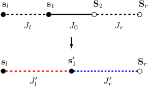
Figure 3: Decimation procedure for a mixed-spin pair according to the second approach.

Since the effective perturbative term introduces spin-$\frac{1}{2}$ objects, one needs to deal with renormalization steps involving both spin-$1$ and spin-$1\over 2$ operators in order to have a closed scheme for the renormalization group.

There is clearly the possibility that the largest local energy scale is set by a pair composed of a spin-$1\over 2$ object $\mathbf{s}_{1}$ and a spin-$1$ object $\mathbf{S}_{2}$ connected by a bond $J_{0}$, and interacting with neighboring spins $\mathbf{s}_{l}$ and $\mathbf{S}_{r}$ via weaker bonds $J_{l}$ and $J_{r}$, as shown in Fig. 3. The ground state of the pair corresponds to a doublet, giving rise to an effective spin-$1\over 2$ object $\mathbf{s}_{1}^{\prime}$, and to first order in perturbation theory the four-spin cluster can be described by an effective Hamiltonian

$$h^{\mathrm{eff}}=J_{l}^{\prime}\mathbf{s}_{l}\cdot\mathbf{s}_{1}^{\prime}+J_{r}^{\prime}\mathbf{s}_{1}^{\prime}\cdot\mathbf{S}_{r},$$ (14)

with

$$J_{l}^{\prime}=-\frac{1}{3}J_{l}\qquad\mbox{and}\qquad J_{r}^{\prime}=\frac{4}{3}J_{r}.$$ (15)

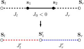
Figure 4: Decimation procedure for a pair of ferromagnetically coupled spin-$1\over 2$ objects according to the second approach.

Notice that this last process generates ferromagnetic bonds, but these only connect spin-$1\over 2$ objects. In case the local energy scale is set by such a bond, $-\left|J_{0}\right|$, connecting $\mathbf{s}_{1}$ and $\mathbf{s}_{2}$, the unperturbed ground state is a triplet, giving rise to an effective spin-$1$ object $\mathbf{S}_{1}^{\prime}$; see Fig. 4. A first-order perturbative calculation leads to an effective Hamiltonian

$$h^{\mathrm{eff}}=J_{l}^{\prime}\mathbf{S}_{l}\cdot\mathbf{S}_{1}^{\prime}+J_{r}^{\prime}\mathbf{S}_{1}^{\prime}\cdot\mathbf{S}_{r},\quad\mbox{with}\quad J_{l,r}^{\prime}=\frac{1}{2}J_{l,r}.$$ (16)

To summarize, in this second approach there are four kinds of bonds, and each of them requires a different decimation rule. In the same notation used in Ref. monthus98, , these are:

(i) Rule 1: A pair of $S={1\over 2}$ spins connected by an ferromagnetic bond [Fig. 4, Eq. (16)];

(ii) Rule 2: A pair of $S={1\over 2}$ spins connected by an antiferromagnetic bond [Fig. 1, Eqs. (4) and (5)];

(iii) Rule 3: A mixed-spin pair connected by an antiferromagnetic bond [Fig. 3, Eqs. (14) and (15)];

(iv) Rule 4: A pair of $S=1$ spins connected by an antiferromagnetic bond [Fig. 2, Eq. (11)].

Which rule is to be applied depends on which bond sets the energy scale at a given step of the SDRG scheme. Using as an estimate for such a scale the local gap $\Delta$ between the ground state and the first discarded excited energy level of the spin pair, we have for the different rules

$$\Delta_{1} = -J_{0}=|J_{0}|,$$

$$\Delta_{2} = J_{0},$$

$$\Delta_{3} = \tfrac{3}{2}J_{0},$$

$$\Delta_{4} = 3J_{0}.$$ (17)

The SDRG scheme for the random-bond spin-$1$ chain then amounts to recursively looking for the bond associated with the largest $\Delta$ and applying the corresponding decimation rule.

In the case of deterministic aperiodicity generated by substitution rules, there appear blocks composed of more than one strong bond, as in the Fibonacci sequence ($abaababaabaab\dots$) with $J_{a}>J_{b}$. In order to deal with these cases, the set of decimation rules has to be extended, as described, in the spin-$1\over 2$ case, in Refs. vieira05a, ; vieira05b, . The starting point is to find the spin block yielding the largest local energy gap, and renormalizing it to either an effective bond between the spins neighboring the block, or to one or two effective spins, according to the lowest energy levels of the original block; see App. B. The effective couplings are then to be calculated by first- or second-order perturbation theory. In order to avoid such complications as much as possible, we choose $J_{b}>J_{a}$ and focus on the strong-modulation regime for analytical calculations. Moderate modulation can be studied numerically using SDRG, by implementing the rules for different blocks, and results from such calculations are briefly mentioned below.

III.3 The third approach

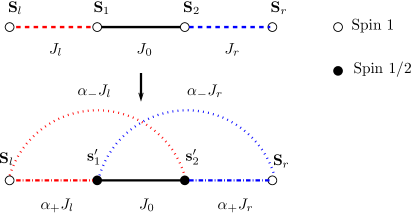
Figure 5: Decimation procedure for a pair of $S=1$ spins according to the third approach.

The third approach consists in using the exact first-order Hamiltonian $h_{1}^{\mathrm{exact}}$ of Eq. (12) as the effective local Hamiltonian that arises from the decimation of a spin-$1$ pair. Among the decimation rules, of concern here is a modification of rule 4 along the lines of Eq. (12). With the introduction of both nearest- and next-nearest-neighbor bonds, it is possible that a spin $\mathbf{S}_{1}$ is strongly coupled to a spin $\mathbf{S}_{2}$ while both are weakly coupled to a number of other spins. Therefore, the exact first-order Hamiltonian turns into

$$h_{1}^{\mathrm{exact}} = \sum_{i=1}^{n_{l}}J_{l}^{(i)}\mathbf{S}_{l}^{(i)}\cdot\left(\alpha_{+}\mathbf{s}_{1}^{\prime}+\alpha_{-}\mathbf{s}_{2}^{\prime}\right)$$ (18)

$$+ \sum_{i=1}^{n_{r}}J_{r}^{(i)}\left(\alpha_{-}\mathbf{s}_{1}^{\prime}+\alpha_{+}\mathbf{s}_{2}^{\prime}\right)\cdot\mathbf{S}_{r}^{(i)},$$

where $n_{l}$ is the number of spins $\mathbf{S}_{l}^{(i)}$ to which $\mathbf{S}_{1}$ is weakly coupled via $J_{l}^{(i)}$, and $n_{r}$ is the number of spins $\mathbf{S}_{r}^{(i)}$ to which $\mathbf{S}_{2}$ is weakly coupled via $J_{r}^{(i)}$. Thus, rule 4 now reads

(iv’) Rule $4^{\prime}$: A pair of $S=1$ spins connected by an antiferromagnetic bond [Fig. 5, Eq. (18)]. Notice that Fig. 5 illustrates the case $n_{l}=n_{r}=1$.

IV The spin-$1$ Fibonacci-Heisenberg chain

The Fibonacci sequence is produced by the iterative application of the substitution rule

$$\sigma_{\textrm{fb}}:\left\{\begin{array}[]{l}a\to ab\\ b\to a\end{array}\right.,$$ (19)

starting from a single letter (either $a$ or $b$).

The spin-$1\over 2$ Heisenberg chain with couplings $J_{i}\in\{J_{a},J_{b}\}$ following the Fibonacci sequence remains critical (i.e. gapless) for all finite values of the coupling ratio $J_{b}/J_{a}$. Since enforced dimerization makes the chain gapped, for general aperiodic sequences the relevant geometric fluctuations to be measured are those associated with pairs of subsequent letters. As discussed in Ref. vieira05b, (and references therein), these grow with the chain length as a power-law, with a wandering exponent $\omega$ related to the substitution rule for letter pairs, rather than for single letters. (For an example concerning the Fibonacci sequence, see App. A )

In the case of the Fibonacci sequence, this exponent is $\omega=0$, in contrast to the random-bond chain, for which $\omega={1\over 2}$. Thus, geometric fluctuations associated with couplings chosen from the Fibonacci sequence are much weaker than those produced by a random coupling distribution. Despite this fact, Fibonacci couplings also induce dramatic changes in the low-temperature behavior of the Heisenberg spin-$1\over 2$ chain.vieira05a ; vieira05b As we show below, this is not the case for the Heisenberg spin-$1$ chain.

In the following sections, we present the results of applying the three different SDRG approaches defined in the previous section to the problem of the Fibonacci-Heisenberg spin-$1$ chain. We also discuss the discrepancies between the second and the other two approaches, and present results from quantum Monte Carlo and DMRG calculations, which point to the fact that, in contrast to the random-bond chain, the second approach does lead to qualitatively incorrect conclusions about the low-temperature behavior of the system.

IV.1 SDRG: The first approach

Figure 6(a) shows the first few bonds near the left end of the Fibonacci-Heisenberg chain. As mentioned before, throughout the paper we assume $J_{b}>J_{a}$, but here, in order to apply the first approach, we assume the stronger condition $J_{b}\gg J_{a}$.

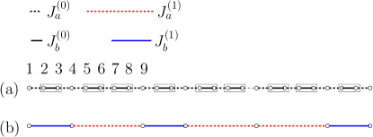
Figure 6: (a) Coupling distribution of the spin-$1$ Fibonacci-Heisenberg chain. (b) Effective chain obtained from the first SDRG approach after a single lattice sweep.

According to the usual recipe of the first approach, all $J_{b}$ bonds, which appear enclosed in Fig. 6(a), are to be decimated in a first SDRG lattice sweep, giving rise to effective couplings. Between spins 1 and 4 in Fig. 6(a) there is one spin pair connected by an isolated $J_{b}$ bond, and its decimation results in an effective bond $J_{b}^{\prime}$, by directly applying Eq. (8). But there is also another effective bond, $J_{a}^{\prime}$, which appears for instance between spins 4 and 9 by sequentially decimating the $J_{b}$ bonds connecting spins $5$-$6$ and $7$-$8$. Thus we have

$$J_{a}^{\prime}=\left(\frac{4}{3}\right)^{2}\frac{J_{a}^{3}}{J_{b}^{2}}\quad\mbox{and}\quad J_{b}^{\prime}=\frac{4}{3}\frac{J_{a}^{2}}{J_{b}}.$$ (20)

Notice that if the effective bond $J_{b}^{\prime}$ is to be smaller than the original bond $J_{b}$, so that the decimations lead to a reduction of the energy scale, we must have $J_{b}>\sqrt{4/3}J_{a}$, which constitutes a consistency condition for the first approach.

As hinted by Fig. 6(b), decimating all original $J_{b}$ bonds leads to a Fibonacci modulation of the effective bonds (disregarding the first effective bond as a boundary effect). It is then clear that a new SDRG sweep will again generate a Fibonacci sequence, and so on. Therefore we can define recursive equations for the effective parameters, as well as for the ratio between them. These are given by

$$J_{a}^{(j+1)} = \left(\frac{4}{3}\right)^{2}\frac{\left[J_{a}^{(j)}\right]^{3}}{\left[J_{b}^{(j)}\right]^{2}},\quad J_{b}^{(j+1)}=\frac{4}{3}\frac{\left[J_{a}^{(j)}\right]^{2}}{J_{b}^{(j)}},$$

$$r^{(j+1)} \equiv \frac{J_{b}^{(j+1)}}{J_{a}^{(j+1)}}=\left(\frac{3}{4}\right)r^{(j)},$$ (21)

in which $j$ labels the SDRG lattice sweep, $j=0$ corresponding to the original chain.

Notice that the ratio between the effective bonds decreases along the RG iterations. This means that the effective chain looks more and more uniform as the energy scale is reduced, and we then conclude that a Fibonacci modulation does not drive the system towards an aperiodic singlet phase even for an arbitrarily large initial coupling ratio, unlike what is observed for the Fibonacci-Heisenberg spin-$1\over 2$ chain.vieira05a ; vieira05b

Thus we expect the chain to remain in the Haldane phase, but with a gap which depends on the bare coupling ratio $r=J_{b}/J_{a}$. An estimate of this gap is provided by the value of the effective couplings at the energy scale for which the effective coupling ratio becomes of order $1$. This happens after $j^{*}$ iterations of the SDRG scheme, with

$$j^{*}=\frac{\ln r}{\ln\frac{4}{3}}.$$ (22)

From the above equations, we thus conclude that the gap should behave as

$$\Delta\left(r\right)\sim r^{-\frac{\ln r}{\ln(4/3)}}J_{b},$$ (23)

up to a multiplicative constant. Taking logarithms on both sides, this last result can be rewritten as

$$\ln\Delta\left(r\right)\sim\ln J_{b}-\frac{\ln^{2}r}{\ln(4/3)},$$ (24)

making evident that the gap vanishes asymptotically as the bare coupling ratio becomes larger and larger, with $J_{b}$ held constant.

It is also possible to follow the growth of bond lengths as the SDRG scheme proceeds. If we denote by $\ell_{a}^{(j)}$ and $\ell_{b}^{(j)}$ the respective lengths of the weak and strong bonds after $j$ SDRG lattice sweeps, inspection of Fig. 6 leads to relations which can be written in matrix form as

$$\left[\begin{array}[]{c}\ell_{a}^{(j+1)}\\ \ell_{b}^{(j+1)}\\ \end{array}\right]=\left[\begin{array}[]{cc}3&2\\ 2&1\\ \end{array}\right]\cdot\left[\begin{array}[]{c}\ell_{a}^{(j)}\\ \ell_{b}^{(j)}\\ \end{array}\right],$$ (31)

so that the asymptotic growth of the bond lengths follows

$$\ell_{a}^{(j)}\sim\ell_{b}^{(j)}\sim\tau^{j},$$ (32)

with $\tau=2+\sqrt{5}$, the largest eigenvalue of the above matrix, corresponding to the rescaling factor of the renormalization-group transformation. Taking into account the bare lengths $\ell_{a}^{(0)}=\ell_{b}^{(0)}=1$, the asymptotic length of the strong bonds is given by

$$\ell_{b}^{(j)}\simeq\frac{1+\sqrt{5}}{2\sqrt{5}}\tau^{j}\equiv c\tau^{j}.$$ (33)

An estimate for the correlation length of the spin-$1$ Fibonacci-Heisenberg chain is provided by the length of the strong bonds at the SDRG iteration where the effective coupling ratio becomes of order 1. Thus, we have

$$\xi\sim\ell_{b}^{\left(j^{*}\right)}\simeq cr^{\nu},$$ (34)

showing that the correlation length diverges at the infinite-modulation limit as a power law with a quite large exponent

$$\nu=\frac{\ln\tau}{\ln{\frac{4}{3}}}\simeq 5.02.$$ (35)

IV.2 SDRG: The second approach

Now we study the conclusions we can extract from the second approach by applying it to the strong-modulation case $J_{b}\gg J_{a}$.

Figure 7 pictures the steps required to obtain effective couplings in the Fibonacci-Heisenberg chain according to the second approach. The original chain is shown in Fig. 7(a). Applying rule 4 of Sec. III.2 to all $J_{b}$ bonds connecting spin-$1$ pairs, these are replaced by spin-$1\over 2$ pairs, as shown in Fig. 7(b). As we assume $J_{b}\gg J_{a}$, the next step involves decimating all $J_{b}$ bonds connecting spin-$1\over 2$ pairs, yielding effective couplings

$$J_{a}^{\prime}=\left(\frac{1}{2}\right)^{2}\frac{J_{a}^{3}}{J_{b}^{2}}\quad\mbox{and}\quad J_{b}^{\prime}=\frac{1}{2}\frac{J_{a}^{2}}{J_{b}}.$$ (36)

Again, ignoring the leftmost bond in Fig. 7(c), the effective couplings follow a Fibonacci sequence.

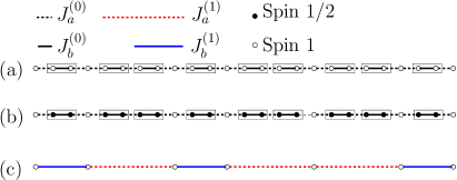
Figure 7: Renormalization of the spin-$1$ Fibonacci-Heisenberg chain according to the second SDRG approach. (a) The original chain. (b) Spin-$1$ pairs connected by (strong) $J_{b}$ bonds are replaced by spin-$1\over 2$ pairs. (c) Spin-$1\over 2$ pairs are decimated, yielding effective couplings between remaining $S=1$ spins.

From the above equations, it is clear that the values of the effective couplings predicted by the second approach are significantly smaller than the ones predicted by the first approach. This fact leads to errors when using effective $J_{b}$ couplings to estimate the energy levels of the Fibonacci-Heisenberg chain, but also, in contrast to the first approach, it is clear that the effective coupling ratio predicted by the second approach,

$$r^{\prime}=\frac{J_{b}^{\prime}}{J_{a}^{\prime}}=2\frac{J_{b}}{J_{a}}=2r,$$ (37)

is larger than the bare coupling ratio $r$. Therefore, according to the second approach, the effective coupling ratio should become larger and larger as the SDRG scheme is iterated, so that Fibonacci-modulated couplings should induce an aperiodicity-dominated gapless phase analogous to the one observed for the Fibonacci-Heisenberg spin-$1\over 2$ chain. This conclusion is qualitatively incorrect, since, as we will see below, taking into account the next-nearest-neighbor bonds neglected in the second approach recovers the predictions of the first approach for strong modulation.

IV.3 SDRG: The third approach

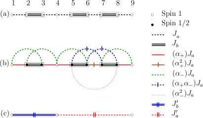
Figure 8: Renormalization of the spin-$1$ Fibonacci-Heisenberg chain according to the third SDRG approach. (a) The original chain. (b) Spin-$1$ pairs connected by (strong) $J_{b}$ bonds are replaced by spin-$1\over 2$ pairs, are further-neighbor couplings are produced. (c) Spin-$1\over 2$ pairs are decimated, yielding effective couplings between remaining $S=1$ spins.

When applying the third approach to the Fibonacci-Heisenberg chain following the recipe of Secs. III.2 and III.3, after replacing all spin-$1$ pairs connected by $J_{b}$ bonds by spin-$1\over 2$ pairs, there appear next-nearest- and further-neighbor bonds as illustrated in Fig. 8(b). In particular, the coupling between spins $5$ and $8$ in Fig. 8(b) appears due to the repeated application of rule $4^{\prime}$.

For $J_{b}>\alpha_{+}^{2}J_{a}\simeq 1.73\,J_{a}$, the largest local gap in Fig. 8(b) is provided by the nearest-neighbor $J_{b}$ bonds (see App. B), which should then be decimated to yield the effective couplings shown in Fig. 8(c). This procedure is different for the $J_{b}$ bonds which are separated from other $J_{b}$ bonds by at least two weaker $J_{a}$ bonds (such as the bond between spins 2 and 3 in the figure) and for the $J_{b}$ bonds separated by a single $J_{a}$ bond (as in the sequence of bonds between spins 5 and 8).

In the former, case we have to treat all weaker bonds (nearest and next-nearest) as perturbations over the Hamiltonian

$$h_{0}=J_{b}\mathbf{s}_{2}\cdot\mathbf{s}_{3},$$ (38)

following a second-order perturbative approach analogous to the one in Eq. (4). The result is an effective bond between spins 1 and 4 in Fig. 8, given by

$$J_{b}^{\prime}=\frac{\left(\alpha_{+}-\alpha_{-}\right)^{2}}{2}\frac{J_{a}^{2}}{J_{b}}=\frac{4}{3}\frac{J_{a}^{2}}{J_{b}}.$$ (39)

In the latter case, so that we avoid ambiguities arising from the order in which the $J_{b}$ bonds are decimated, we must perform a third-order perturbative calculation in which all weaker bonds (nearest and next-nearest) are treated as perturbations over the Hamiltonian

$$h_{0}=J_{b}\mathbf{s}_{5}\cdot\mathbf{s}_{6}+J_{b}\mathbf{s}_{7}\cdot\mathbf{s}_{8}.$$ (40)

As detailed in App. C, this yields an effective bond connecting spins 4 and 9, given by

$$J_{a}^{\prime}=\frac{\left(\alpha_{+}-\alpha_{-}\right)^{4}}{4}\frac{J_{a}^{3}}{J_{b}^{2}}=\left(\frac{4}{3}\right)^{2}\frac{J_{a}^{3}}{J_{b}^{2}}.$$ (41)

Thus, comparing the above results with Eq. (20), we see that for $J_{b}>\alpha_{+}^{2}J_{a}$ the third approach yields exactly the same effective bonds as the first approach. Therefore, properly taking into account next-nearest neighbor bonds generated by the SDRG scheme fixes the qualitatively incorrect prediction of the second approach that strong Fibonacci modulations induce a gapless, aperiodicity-dominated phase in the Heisenberg spin-$1$ chain.

For weaker coupling ratios, $1<J_{b}/J_{a}<\alpha_{+}^{2}$, the largest local gap in Fig. 8(b) is not set by the $J_{b}$ bonds, and the order of the decimations is altered. Numerical implementations of the third approach indicate that the distribution of effective bonds becomes dimerized. As it is known that a dimerized spin-$1\over 2$ chain has a ground state which is adiabatically connected to the Haldane phasehida92 , this is in qualitative agreement with the prediction of the first approach, and with the fact that the Haldane phase is stable towards Fibonacci modulations for any value of the coupling ratio.

IV.4 Comparison with QMC simulations

According to the SDRG predictions, for strong modulation ($r\gg 1$), the Fibonacci-Heisenberg chain can be approximated as a collection of independent spin pairs, coupled in singlet states by the effective $J_{b}$ bonds. In the spin-$1\over 2$ case, for which the ground state is expected to be in the aperiodic singlet phase,vieira05b this picture should be qualitatively correct at all temperatures, provided the modulation is strong enough. On the other hand, in the spin-$1$ case, this picture should break down at temperatures below the energy gap $\Delta\left(r\right)$ of Eq. (23). Therefore, we can estimate the free energy of the Fibonacci-Heisenberg chain as

$$f(B,T)=\frac{1}{2}\sum\limits_{j=0}^{j^{*}}(n_{j}-n_{j+1})F_{\mathrm{pair}}\left(J_{b}^{(j)};B,T\right),$$ (42)

where $F_{\mathrm{pair}}\left(J_{b}^{(j)};B,T\right)$ is the free energy of a spin pair interacting via the Hamiltonian

$$H_{\mathrm{pair}}=J_{b}^{(j)}\mathbf{S}_{1}\cdot\mathbf{S}_{2}-B(S_{1}^{z}+S_{2}^{z})$$ (43)

(with $B$ a small magnetic field, introduced to allow the calculation of the magnetic susceptibility), $n_{j}$ is the fraction of active spins (those not yet decimated) at the $j$-th iteration of the SDRG scheme, and $j^{*}$ is the iteration at which the effective coupling ratio becomes of order unity. From the above discussion, it is clear that $j^{*}=\infty$ for the spin-$1\over 2$ case, while it can be shown from Eqs. (21) that $j^{*}=\ln r/\ln\left(4/3\right)$ for the spin-$1$ case.

For the first $j^{*}$ iterations of the SDRG scheme, as the effective couplings always follow a Fibonacci sequence, the fraction of active spins satisfy the recurrence relation $n_{j+1}=(1-2f_{b})n_{j}$, where $f_{b}=(3-\sqrt{5})/2\simeq 0.382$ is the fraction of letters $b$ in the infinite Fibonacci sequence (see App. D). Thus, we obtain $n_{j}=(1-2f_{b})^{j}$.

The susceptibility at zero field is readily obtained from the free energy,

$$\chi(T)=-\left.\frac{\partial^{2}f}{\partial B^{2}}\right|_{B=0}.$$ (44)

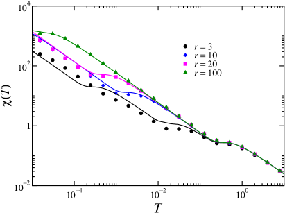
Figure 9: Magnetic susceptibility as a function of temperature for the spin-1/2 Fibonacci-Heisenberg chain. Solid lines correspond to the SDRG prediction for different coupling ratios $r=J_{b}/J_{a}$. QMC results (symbols) were obtained using chains with 90 sites and open boundary conditions. Error bars are smaller than symbol size.

We first checked the SDRG predictions for the spin-$1\over 2$ chain, using the effective couplings calculated in Ref. vieira05b, , by comparing the results of Eqs. (42) and (44) with QMC simulations, performed using the stochastic series expansion scheme Sandvik91 ; Sandvik92 with directed loop updates Syljuasen02 . As shown in Fig. 9, the SDRG prediction gets closer and closer to the QMC results as the modulation increases, as expected from the perturbative nature of the SDRG scheme.

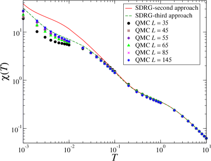
Figure 10: Temperature dependence of the magnetic susceptibility for the spin-$1$ Fibonacci-Heisenberg chain with coupling ratio $r=10$. Solid (dashed) line corresponds to the SDRG prediction according to the second (third) approach, while symbols correspond to QMC results for different chain sizes $L$. QMC error bars are smaller than symbol size.

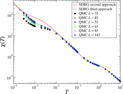
Figure 11: Temperature dependence of the magnetic susceptibility for the spin-$1$ Fibonacci-Heisenberg chain, similar as Fig. 10, but with a coupling ratio $r=20$.

For the corresponding spin-$1$ chain, Figs. 10 and 11 show the temperature dependence of the susceptibility according to the second and third SDRG approaches, along with QMC data, for coupling ratios $r=10$ and $r=20$, respectively. Clearly, the agreement with low-temperature numerical data is significantly better for the third SDRG approach, and improves as the number $L$ of spins in the chain increases. Notice the shoulders in the susceptibility curves (e.g., slightly to the left of $T\simeq 10^{0}$ and $10^{-2}$ in Fig. 10) at temperatures close to energy scales related to the effective $J_{b}$ bonds.

As the QMC calculations involve chains with an odd number of spins, the susceptibility does not vanish at low temperatures even when the ground state is gapped. However, for the coupling ratios used in Figs. 10 and 11, the energy scale of the gaps, according to Eq. (23), correspond to temperatures below $10^{-8}J_{b}$, much lower than the temperatures that could be reached in our simulations.

IV.5 Gap and string order correlations of the Fibonacci $S=1$ chain as a function of the coupling ratio

In order to check whether a sufficiently large coupling ratio could induce a gapless aperiodic singlet phase, we now present a numerical determination of the spin gap for different values of the coupling ratio and different chains lengths, using the DMRG method.

DMRG simulation details. We simulate aperiodic $S=1$ chains with a number $L$ of spins, with open boundary conditions, using DMRG white92 formulated in the matrix-product state formalism McCulloch07 . We use an SU$(2)$-symmetric formulation McCulloch02 , taking advantage of the symmetry of the Hamiltonian (1), which reduces considerably the number of states $m$ to be kept in the DMRG calculation. We nevertheless find that the convergence to the ground states in different total spin sector $S_{T}=0,1$ or $2$ is particularly difficult to achieve for large $L$ and large coupling ratio $r$, which we attribute to the aperiodicity in the system. To ensure convergence, we use a specific warming procedure where we increase sequentially the number $m$ of SU$(2)$ states kept, typically by values of $20$ or $50$, up to values of $m$ where the ground-state energy no longer varies. For the largest Fibonacci chains (here $L=378$), the maximum number of SU$(2)$ states was $m=1000$, corresponding to approximatively $4800$ U$(1)$ states. For each value of $m$ in this warming procedure, we perform a very large (sometimes more than $200$) number of sweeps, again checking that the energy does not vary.

Numerical determination of gaps. Depending on the parity of the chain size $L$, the ground-state is found to be in the $S_{T}=0$ sector (for even $L$) or the $S_{T}=1$ sector (odd $L$), as expected. In the Haldane phase, the energy difference between these two sectors is expected to decrease exponentially with increasing $L$ for open chains, due to the presence of spin-$\frac{1}{2}$ degrees of freedom near the boundaries. Similar to what was done in the original DMRG study of uniform $S=1$ chains white92 , we compute the gap $\Delta$ as the energy difference between this ground-state and the energy of the ground-state in the $S_{T}=2$ sector: $\Delta=E_{0}(S_{T}=2)-E_{0}(S_{T}=0/1)$. We simulate chains with sizes $L=14,22,35,56,90,145,234,378$ corresponding to the “natural” numbers (in the Fibonacci sequence) of bonds $L-1=13,21,34,55,89,144,233,377$. In the following, results are presented only for the specific Fibonacci bond sequence corresponding to the size $L$ and starting with a single letter $a$, but we checked for small $L<70$ that the same qualitative behavior is obtained when averaging results over the $L+1$ different possible subsequences of the Fibonacci sequence that can be accommodated in a chain with $L$ spins.

We present in Fig. 12 the results for the gap $\Delta$ (in units of $J_{a}$), as a function of coupling ratio $r$, for different system sizes $L$. It is clear from this figure that the gap does not vanish in the entire range $r\in[1,6]$ that we simulated, even though as expected, it decreases quite considerably with increasing $r$.

Notice that we should not expect the DMRG gaps to be direcly comparable to those predicted by Eq. (23), which is valid in the infinite-chain, large-modulation limit, and disregards boundary effects. These turn out to be quite important, especially for the small chain lengths accessible via DMRG. Instead, we present in the inset of Fig. 12 a comparison between the DMRG gaps for the strongest modulation for which reliable data are available, $r=6$, and the corresponding open-chain SDRG predictions (see App. E). The agreement is quite good for small chains, but discrepancies arise for $L\geq 56$, due to the fact that, as the effective coupling ratio decreases for increasing system size [see Eq. (21)], the perturbative calculations underlying the SDRG approach become less precise, leading to errors in the gap estimate. Nevertheless, for still larger chains ($L=234$ and $L=378$), the curves clearly approach each other.

String order. The previous gap results indicate that the Haldane phase is not destroyed by imposing a Fibonnaci aperiodic sequence for the couplings. This is furthermore confirmed by the numerical DMRG computation of the string order correlation function, dennijs

$$\langle O^{z}(i,j)\rangle=\langle S^{z}_{i}\exp(\i\pi\prod_{k=i+1}^{j-1}S^{z}_{k})S^{z}_{j}\rangle,$$

as a function of the distance $x=|j-i|$. The string order correlation function takes non-vanishing values in the large distance limit in the Haldane phase dennijs and is thus a good indicator of the continuity of the Haldane phase as the strength of the aperiodicity is increased. We represent in Fig. 13 $\langle O^{z}(x=|j-i|)\rangle$ with $i=L/4$ and $x$ running from $0$ to $L/2$ (we consider the initial and final points to minimize effects due to the open boundary conditions) for selected values of the coupling ratio $r$, for the largest $L=378$ system simulated. A real-space correlation function such as $\langle O^{z}(x)\rangle$ is inevitably non-monotonous for such aperiodic systems, but the results of Fig. 13 indicate that the string order does not vanish up to $r=6$, albeit it reaches smaller thermodynamic values (when $x\rightarrow\infty$) as $r$ is increased, as expected from the gap behavior.

Overall, the DMRG results on the gap and string order support the conclusion of SDRG (approaches $1$ and $3$) that the gapped Haldane phase remains robust against Fibonacci aperiodicity.

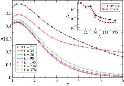
Figure 12: Spin $1$ chain modulated by the Fibonacci sequence: gap $\Delta=E_{0}(S_{T}=2)-E_{0}(S_{T}=0/1)$ between the lowest-lying quintuplet $S_{T}=2$ state energy $E_{0}(S_{T}=2)$ and the ground-state energy $E_{0}$ (which is either in the $S_{T}=0$ singlet or $S_{T}=1$ triplet sector, depending on the chain parity), as a function of coupling ratio $r=J_{b}/J_{a}$, for different system sizes $L$.

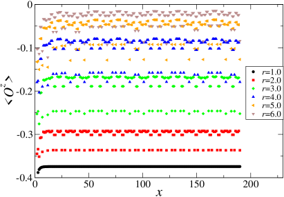
Figure 13: Spin $1$ chain modulated by the Fibonacci sequence: string order correlation function $\langle O^{z}(x=|i-j|)\rangle$ as a function of distance $x$ taken starting from the quarter-chain point $i=L/4$ up to the maximum value $x=L/2$, for a $L=376$ chain and different aperiodicity strengths $r=J_{b}/J_{a}$.

V The spin-$1$ chain with couplings following the 6-3 sequence

We now study the effects of geometric fluctuations induced by couplings following the 6-3 sequence on the spin-$1$ Heisenberg chain. The 6-3 sequence is defined by the substitution rule

$$\sigma_{63}:\left\{\begin{array}[]{l}a\to babaaa\\ b\to baa\end{array}\right.,$$ (45)

starting from a single letter (either $a$ or $b$). The wandering exponent characterizing pair fluctuations in the 6-3 sequencevieira05b is $\omega=\ln 2/\ln 5\simeq 0.43$, and thus we expect for the spin-$1\over 2$ chain and for the strong-modulation spin-$1$ chain a dynamical scaling characterized by the stretched exponential form

$$\Delta\left(\ell\right)\sim\exp\left(\ell/\ell_{0}\right)^{\omega},$$ (46)

with $r_{0}$ a nonuniversal constant. As described below, this is exactly what we obtain from the SDRG scheme.

V.1 The first approach

Figure 14(a) shows the bond distribution prescribed by the 6-3 sequence. Assuming again $J_{b}>J_{a}$, the first SDRG lattice sweep generates two kinds of effective bonds, exactly as in the case of the Fibonacci-Heisenberg chain (see Fig. 6). Furthermore, the remaining $J_{a}$ couplings can be reinterpreted as a third kind of effective bond, so that we can write

$$J_{1}^{(0)}=J_{a},\quad J_{2}^{(0)}=\left(\frac{4}{3}\right)\frac{J_{a}^{2}}{J_{b}},\quad J_{3}^{(0)}=\left(\frac{4}{3}\right)^{2}\frac{J_{a}^{3}}{J_{b}^{2}},$$ (47)

as long as $J_{b}>\sqrt{4/3}J_{a}$.

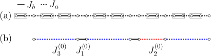
Figure 14: (a) Coupling distribution of the spin-$1$ Heisenberg chain according to the 6-3 sequence. (b) Effective chain obtained from the first SDRG approach after a single lattice sweep.

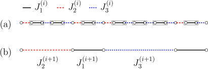
Figure 15: Self-similar coupling distribution obtained from the first SDRG approach for subsequent lattice sweeps. Singlets are formed between spins connected by the strong effective bonds $J_{1}^{(i)}$.

Subsequent SDRG lattice sweeps yield a scale-invariant coupling distribution, as shown in Fig. 15, leading to a set of recurrence equations given by

$$J_{1}^{(j+1)} = \left(\frac{4}{3}\right)\frac{J_{2}^{(j)}J_{3}^{(j)}}{J_{1}^{(j)}},\quad J_{2}^{(j+1)}=\left(\frac{4}{3}\right)^{2}\frac{J_{2}^{(j)}\left[J_{3}^{(j)}\right]^{2}}{\left[J_{1}^{(j)}\right]^{2}},$$

$$J_{3}^{(j+1)} = \left(\frac{4}{3}\right)^{3}\frac{J_{2}^{(j)}\left[J_{3}^{(j)}\right]^{3}}{\left[J_{1}^{(j)}\right]^{3}},$$ (48)

which are valid as long as $J_{1}^{(j)}>J_{2}^{(j)}$. This last condition is true only for $J_{b}>(4/3)J_{a}$.

Defining coupling ratios between the parameters $J_{1}$, $J_{2}$ and $J_{3}$, we can write the recurrence equations

$$\rho^{(j+1)} \equiv \frac{J_{1}^{(j+1)}}{J_{3}^{(j+1)}}=\left[\frac{3}{4}\rho^{(j)}\right]^{2},$$

$$\sigma^{(j+1)} \equiv \frac{J_{1}^{(j+1)}}{J_{2}^{(j+1)}}=\frac{3}{4}\rho^{(j)},$$ (49)

making it clear that, under the condition $J_{b}>(4/3)J_{a}$, there is a single, infinite-modulation fixed point, $\rho^{\infty}=\sigma^{\infty}=\infty$. Thus, the first SDRG approach predicts that, in the strong-modulation limit, couplings following the 6-3 sequence induce a gapless aperiodic singlet phase, whose dynamical scaling form is calculated in Sec. V.4. A rough estimate of the critical point separating the Haldane phase from the gapless phase is provided by the condition $J_{b}>(4/3)J_{a}$.

V.2 The second approach

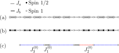
Figure 16: First step of renormalization of the spin-$1$ Heisenberg chain with couplings following the 6-3 sequence according to the second SDRG approach. (a) The original chain. (b) Spin-$1$ pairs connected by (strong) $J_{b}$ bonds are replaced by spin-$1\over 2$ pairs. (c) Spin-$1\over 2$ pairs are decimated, yielding effective couplings between remaining $S=1$ spins.

Figure 16 shows the results of applying the second SDRG approach to the spin-$1$ Heisenberg chain with couplings modulated by the 6-3 sequence. In Fig. 16(b), all spin pairs connected by $J_{b}$ bonds are replaced by spin-$1\over 2$ pairs after the first lattice sweep, and for $J_{b}\gtrsim 1.91\,J_{a}$ all spin-$1\over 2$ pairs are then decimated, leading to the configuration in Fig. 16(c), with three effective bonds given by

$$J_{1}^{(0)}=J_{a},\quad J_{2}^{(0)}=\left(\frac{1}{2}\right)\frac{J_{a}^{2}}{J_{b}},\quad J_{3}^{(0)}=\left(\frac{1}{2}\right)^{2}\frac{J_{a}^{3}}{J_{b}^{2}}.$$ (50)

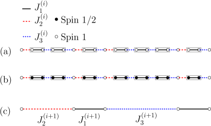
Figure 17: Self-similar coupling distribution obtained from the second SDRG approach for subsequent RG steps. (a) Effective chain consisting only of $S=1$ spins. (b) Strongly connected spin-$1$ pairs form spin-$1\over 2$ pairs. (c) Spin-$1\over 2$ pairs are decimated, giving rise to a new effective chain, again consisting only of spin-$1$ pairs, with an invariant coupling distribution.

Starting from the configuration in Fig. 16(c), each subsequent SDRG steps involve two consecutive sweeps through the lattice, the first one replacing all spin-$1$ pairs connected by $J_{1}$ bonds by spin-$1\over 2$ pairs, which are then decimated to yield new effective couplings. This is illustrated in Fig. 17, and leads to the recurrence relations

$$J_{1}^{(j+1)} = \left(\frac{1}{2}\right)\frac{J_{2}^{(j)}J_{3}^{(j)}}{J_{1}^{(j)}},\quad J_{2}^{(j+1)}=\left(\frac{1}{2}\right)^{2}\frac{J_{2}^{(j)}\left[J_{3}^{(j)}\right]^{2}}{\left[J_{1}^{(j)}\right]^{2}},$$

$$J_{3}^{(j+1)} = \left(\frac{1}{2}\right)^{3}\frac{J_{2}^{(j)}\left[J_{3}^{(j)}\right]^{3}}{\left[J_{1}^{(j)}\right]^{3}},$$ (51)

in which $j$ labels the SDRG step. These equations are valid as long as $J_{1}^{(j)}>\frac{3}{2}J_{2}^{(j)}$, a condition that is always verified for $J_{b}\gtrsim 1.91\,J_{a}$.

As in the case of the first approach, we can define the coupling ratios $\rho\equiv J_{1}/J_{3}$ and $\sigma\equiv J_{1}/J_{2}$, whose recurrence relations read

$$\rho^{(j+1)} = \left[2\rho^{(j)}\right]^{2},$$

$$\sigma^{(j+1)} = 2\rho^{(j)}.$$ (52)

These also point to an infinite-modulation fixed point, $\rho^{\infty}=\sigma^{\infty}=\infty$, so that predictions from the first and the second approach are now in qualitative agreement, although, as for the Fibonacci-Heisenberg chain, the energy levels predicted by the two approaches (estimated from the effective $J_{1}$ bonds) are distinct.

If $J_{b}\lesssim 1.91\,J_{a}$, numerical implementations of the second SDRG approach (not detailed here) predict the renormalization of a different set of bonds than in the first SDRG step, according to the recipe associating the energy scale with the bond clusters yielding the largest local gap. However, for $1.69\,J_{a}\lesssim J_{b}\lesssim 1.91\,J_{a}$, the distribution of effective couplings in Fig. 17(a) is eventually reached, so that the scheme still predicts a gapless, aperiodic singlet phase as the ground state. For $J_{b}\lesssim 1.69\,J_{a}$, however, the distribution of effective couplings arrives at a dimerized spin-$1\over 2$ chain, a state equivalent to the Haldane phase. Thus, within the approximations leading to the second SDRG approach, $J_{b}\simeq 1.69\,J_{a}$ corresponds to the critical point separating a gapped from an aperiodicity-dominated gapless phase.

V.3 The third approach

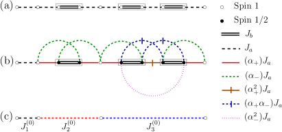
Figure 18: First step of the renormalization of the spin-$1$ Heisenberg chain with couplings following the 6-3 sequence, according to the third SDRG approach. (a) The original chain. (b) Spin-$1$ pairs connected by (strong) $J_{b}$ bonds are replaced by spin-$1\over 2$ pairs, are further-neighbor couplings are produced. (c) Spin-$1\over 2$ pairs are decimated, yielding effective couplings between remaining $S=1$ spins.

Figure 18 shows the first step of the renormalization of the spin-$1$ Heisenberg chain with couplings following the 6-3 sequence, according to the third SDRG approach. Forming spin-$1\over 2$ pairs from strongly connected spin-$1$ pairs, and assuming $J_{b}>3J_{a}$, second- and third-order perturbation theory leads to effective couplings which, along with the remaining $J_{a}$ bonds, define a set of effective bonds

$$J_{1}^{(0)} = J_{a},$$

$$J_{2}^{(0)} = \frac{(\alpha_{+}-\alpha_{-})^{2}}{2}\frac{J_{a}^{2}}{J_{b}}=\left(\frac{4}{3}\right)\frac{J_{a}^{2}}{J_{b}},$$

$$J_{3}^{(0)} = \frac{(\alpha_{+}-\alpha_{-})^{4}}{4}\frac{J_{a}^{3}}{J_{b}^{2}}=\left(\frac{4}{3}\right)^{2}\frac{J_{a}^{3}}{J_{b}^{2}},$$ (53)

exactly as in the first SDRG approach. Notice that, as in the Fibonacci-Heisenberg chain, further-neighbor couplings are introduced in the middle of the RG step, but eliminated at the end for strong enough modulation. Nevertheless, they are essential in obtaining from the third approach the same effective couplings predicted by the first approach.

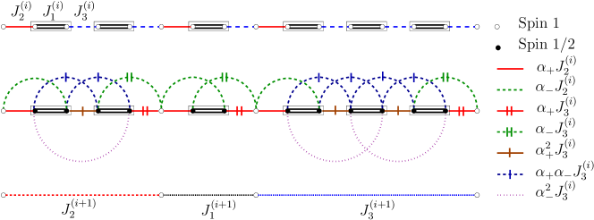
Figure 19: Self-similar coupling distribution obtained from the third SDRG approach for subsequent RG steps. (a) Effective chain consisting only of $S=1$ spins. (b) Strongly-connected spin-$1$ pairs form spin-$1\over 2$ pairs, and further-neighbor bonds are formed. (c) Spin-$1\over 2$ pairs are decimated, giving rise to a new effective chain, again consisting only of spin-$1$ pairs, with an invariant coupling distribution.

Subsequent SDRG steps start from the coupling distribution in Fig. 18(c), shown in expanded form in Fig. 19(a). After forming spin-$1\over 2$ pairs from spin-$1$ pairs coupled by effective $J_{1}$ bonds, these spin-$1\over 2$ pairs are decimated, taking into account the presence of further neighbor bonds, to yield, from second-, third- and fourth-order perturbation theory, new effective couplings obeying the recurrence relations

$$J_{1}^{(j+1)} = \frac{(\alpha_{+}-\alpha_{-})^{2}}{2}\frac{J_{2}^{(j)}J_{3}^{(j)}}{J_{1}^{(j)}}=\left(\frac{4}{3}\right)\frac{J_{2}^{(j)}J_{3}^{(j)}}{J_{1}^{(j)}},$$

$$J_{2}^{(j+1)} = \frac{(\alpha_{+}-\alpha_{-})^{4}}{4}\frac{J_{2}^{(j)}\left[J_{3}^{(j)}\right]^{2}}{\left[J_{1}^{(j)}\right]^{2}}=\left(\frac{4}{3}\right)^{2}\frac{J_{2}^{(j)}\left[J_{3}^{(j)}\right]^{2}}{\left[J_{1}^{(j)}\right]^{2}},$$

$$J_{3}^{(j+1)} = \frac{(\alpha_{+}-\alpha_{-})^{6}}{8}\frac{J_{2}^{(j)}\left[J_{3}^{(j)}\right]^{3}}{\left[J_{1}^{(j)}\right]^{3}}=\left(\frac{4}{3}\right)^{3}\frac{J_{2}^{(j)}\left[J_{3}^{(j)}\right]^{3}}{\left[J_{1}^{(j)}\right]^{3}},$$

valid as long as $J_{b}>\alpha_{+}^{2}Ja$.

Thus, for sufficiently strong modulation, the first and the third SDRG approaches yield the same quantitative predictions for the ground-state properties and the energy levels, while the second approach qualitatively agrees with the other two.

In the presence of moderate or weak modulation, in which the perturbative calculations underlying the SDRG scheme become increasingly inadequate, quantitative predictions are expected to depend on finer details of the first and third approaches. Indeed, for $\alpha_{+}^{2}J_{a}<J_{b}<3J_{a}$, numerical implementations of the third approach still predict a gapless ground state, although with a slightly different set of renormalized bonds in the first RG step. However, for $J_{b}\lesssim\alpha_{+}^{2}J_{a}$, the third approach eventually leads to an effective chain composed of spin-$1\over 2$ objects with a dimerized distribution of effective couplings, thus predicting a gapped phase. Of course, for such a range of coupling ratios, we do not expect any of the predictions for the critical coupling ratio to be precise.

V.4 Dynamic scaling relation

In the strong-modulation gapless phase we can derive the dynamic scaling relation between energy and length scales. It is natural to assume that, as the various energy levels are estimated from the values of the strongest effective couplings at each step of the SDRG scheme, the relevant length scales are the corresponding effective lengths. From the recurrence relations in Eqs. (LABEL:recursive-seq63), and by looking at Fig. 19, it can be seen that the lengths of the effective couplings satisfy recurrence relations that can be written in matrix form as

$$\left[\begin{array}[]{cc}\ell_{1}^{(j+1)}\\ \ell_{2}^{(j+1)}\\ \ell_{3}^{(j+1)}\end{array}\right]=\left[\begin{array}[]{ccc}1&1&1\\ 2&1&2\\ 3&1&3\end{array}\right]\cdot\left[\begin{array}[]{ccc}\ell_{1}^{(j)}\\ \ell_{2}^{(j)}\\ \ell_{3}^{(j)}\end{array}\right],$$ (64)

in which again $j$ labels the SDRG steps. The matrix appearing in the above equation has eigenvalues $\lambda_{1}=\lambda_{2}=0$ and $\lambda_{3}=5$, so that, in the asymptotic limit, all effective lengths scale as

$$\ell^{(j)}\sim\lambda_{3}^{j}.$$ (65)

The energy levels, being proportional to the value of the largest bond in each iteration, scale as $\Delta_{j}\sim J_{1}^{(j)}$. Thus, by solving the recurrence relations in Eqs. (49) and (LABEL:recursive-seq63), we can write

$$\Delta_{j}\sim\ell_{j}^{\frac{-2\ln(4/3)}{\ln 5}}\exp\left[-\frac{3}{2}\ln\left(\frac{9}{16}\rho^{(0)}\right)\ell_{j}^{\omega}\right],$$ (66)

with $\omega=\frac{\ln 2}{\ln 5}$. As expected, apart from unimportant constants, this is the same stretched-exponential form obeyed by the spin-$1\over 2$ Heisenberg chain with couplings following the 6-3 sequence.

V.5 Comparison with QMC simulations

Using the same independent-singlet approximation described for the Fibonacci-Heisenberg chain in Sec. IV.4, we can obtain SDRG predictions for the susceptibility at zero field when couplings follow the 6-3 sequence. Only a small adaptation is necessary, as the self-similar coupling distribution is distinct from the 6-3 sequence itself. Thus, we must take into account that the fraction of $J_{b}$ bonds in the original chain is $f_{b}=\frac{1}{3}$, while the fraction of $J_{1}$ bonds in the self-similar distribution is $f_{J_{1}}=\frac{2}{5}$. Below, the results of the independent-singlet approximation are compared with quantum Monte Carlo simulations.

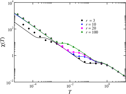
Figure 20: Temperature dependence of the magnetic susceptibility for the spin-$1\over 2$ Heisenberg chain with aperiodic couplings following the 6-3 sequence. Solid lines are the SDRG predictions for various coupling ratios $r=J_{b}/J_{a}$, while symbols indicate the corresponding QMC results obtained for $L=75$ sites.

For the spin-$1\over 2$ chain with $L=75$ sites the results are shown in Fig. 20. As expected, the agreement between the SDRG prediction and QMC simulations is better for larger coupling ratios $r=J_{b}/J_{a}$.

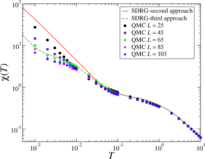
Figure 21: Temperature dependence of the magnetic susceptibility for the spin-$1$ Heisenberg chain with aperiodic couplings following the 6-3 sequence with coupling ratio $r=5$. Solid (dashed) line corresponds to the SDRG prediction according to the second (third) approach, while symbols correspond to QMC results for different chain sizes $L$. QMC error bars are smaller than symbol size.

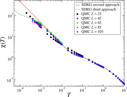
Figure 22: Temperature dependence of the magnetic susceptibility for the spin-$1$ Heisenberg chain with aperiodic couplings following the 6-3 sequence, similar as Fig. 21, but with a coupling ratio $r=10$.

In Figs. 21 and 22 we show the results for the spin-$1$ chain with coupling ratios $r=5$ and $r=10$ respectively. As in the case of the Fibonacci-Heisenberg chain, it is clear that the QMC results are in better agreement with the predictions of the third SDRG approach. Again notice the shoulders in the susceptibility curves close to temperatures corresponding to energy scales related to the effective $J_{b}$ bonds.

V.6 Gap and string order of the 6-3 $S=1$ chain as a function of the coupling ratio

We use the same DMRG procedure described in Sec. IV.5 to compute the spin gap $\Delta$ (in units of $J_{a}$) for open $S=1$ spin chains modulated by the 6-3 sequence. We use systems of sizes $L=45,75,85,105,325,376$ and display the results in Fig. 23. Our calculations reveal that the spin gap $\Delta$ clearly vanishes for sufficiently large systems, when the coupling ratio $r$ is large enough. For the largest systems considered ($L=325$ and $L=376$), our simulations did not converge for too large values of $r\geq 4$, but the behavior at smaller $r$ and for smaller $L$ clearly indicates that the gap must vanish for these cases.

These results are again in agreement with the SDRG calculations, which indicate that the Haldane gap must vanish above a critical modulation $r_{c}$, to give rise to the gapless aperiodic singlet phase. The critical value $r_{c}$ at which this quantum phase transition takes place is difficult to estimate precisely due to strong finite-size effects arising from a small gap. Considering the largest system available, we can nevertheless ascertain that the system is gapless at $r=3.4$. The inset of Fig. 23 displays the spin gap $\Delta$ as a function of inverse system size $1/L$, for values of the coupling ratio close to the transition. We can tentatively deduce a value $r_{c}\approx 2.9(2)$, even though this phenomenological determination has to be taken with care. Even though the SDRG prediction $r_{c}\simeq 1.73$ (from approach $3$) is different, it is subject to a large uncertainty, since for such small values of the bond ratio the perturbative calculations become much imprecise, and we can nevertheless conclude that the numerical calculations of the spin gap support the SDRG prediction of a gapless phase at large enough (but finite) value of the coupling ratio $r$.

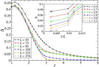
Figure 23: Spin-$1$ chain modulated by the 6-3 sequence: gap $\Delta=E_{0}(S_{T}=2)-E_{0}(S_{T}=0\/1)$ between the lowest-lying quintuplet $S_{T}=2$ state energy $E_{0}(S_{T}=2)$ and the ground-state energy $E_{0}$ (which is either in the $S_{T}=0$ singlet or $S_{T}=1$ triplet sector, depending on the chain parity), as a function of coupling ratio $r=J_{b}/J_{a}$, for different system sizes $L$.

We finally confirm this finding by computing the string order correlation function $\langle O^{z}(x=|j-i|)\rangle$ using the same setup as presented in Sec. IV.5. We present in Fig. 24 the results of our simulations for the maximum chain size $L=376$ where we could reach convergence for $r=1,2,3$ (top panel) and for a smaller chain size $L=105$ where convergence was ensured up to $r=6$ (bottom panel), for integer values of $r$. For $L=376$, the long-distance behavior of $\langle O^{z}(x)\rangle$ indicates that the Haldane phase is still present in this finite-size sample up to $r=3$, albeit with a small string order parameter for this latter value of $r$, in agreement with the small gap value found for this system. On the other hand, for $r=4,5,6$, results for the smaller sample $L=105$ already clearly indicate that the string order vanishes in the long-distance limit, nicely confirming that the Haldane phase has disappeared. Due to the irregular behavior in $x$, we did not attempt to perform finite-size scaling on the string-order correlation function for different system sizes to estimate the critical coupling value $r_{c}$, but our results for the largest sample $L=376$ are consistent with the estimate $r_{c}=2.9(2)$ obtained from the gap estimate.

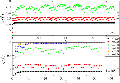
Figure 24: Spin-$1$ chain modulated by the 6-3 sequence: string order correlation function $\langle O^{z}(x=|i-j|)\rangle$ as a function of distance $x$ taken starting from the quarter-chain point $i=L/4$ up to the maximum value $x=L/2$, for a $L=376$ chain (top) and a $L=105$ chain (bottom) and different aperiodicity strengths $r=J_{b}/J_{a}$.

VI Discussion and Conclusions

In this paper, we investigated the effects of aperiodic but deterministic bond modulations on the zero and low-temperature properties of the spin-$1$ Heisenberg chain. We presented explicit results for aperiodic bonds generated by two different binary substitution rules, associated with the Fibonacci and the 6-3 sequences.

For the Fibonacci-Heisenberg chain, whose geometric fluctuations are gauged by a wandering exponent $\omega=0$, calculations based on different adaptations of the SDRG scheme yielded conflicting results. While the SDRG approach of Monthus et al. monthus97 ; monthus98 , which allows for the appearance of effective $S={1\over 2}$ spins as the transformation proceeds, predicts that for strong bond modulation the ground state corresponds to a gapless, aperiodicity-dominated phase, the inclusion of nonfrustrating next-nearest-neighbor effective bonds in the SDRG scheme points to a gapped ground state, and to the stability of the Haldane phase towards any finite Fibonacci modulation. This is the same prediction as obtained from the simplest SDRG scheme which only involves $S=1$ spins, and is supported by both quantum Monte Carlo and DMRG calculations.

On the other hand, for the Heisenberg chains with bonds following the 6-3 sequence, characterized by stronger geometric fluctuations ($\omega\simeq 0.43$), all SDRG approaches give the same qualitative prediction, according to which the Haldane phase should be stable in the presence of weak bond modulation (as measured by the ratio $r$ between the strong and weak bonds $J_{b}$ and $J_{a}$), while strong bond modulation ($r\gg 1$) drives the ground state towards a gapless aperiodicity-dominated phase, similar to the one obtained for the analogous $S={1\over 2}$ Heisenberg chain. Again, this prediction is nicely supported by quantum Monte Carlo and DMRG calculations.

Although we only presented explicit calculations for two aperiodic sequences, we can draw more general conclusions for the strong-modulation regime based on known results for the $S={1\over 2}$ Heisenberg chain. vieira05b For virtually all binary substitution sequences characterized by a wandering exponent $\omega\geq 0$, it is possible to write recursion relations for a main bond ratio in the form vieira05b

$$r^{(j+1)}=\gamma\left[r^{(j)}\right]^{k},$$ (67)

where $\gamma$ is a constant, $r^{(j)}$ is the bond ratio calculated at the $j$th iteration of the SDRG transformation, and $k$ is an integer related to the wandering exponent $\omega$ and to the rescaling factor $\tau$ of the transformation by

$$\omega=\frac{\ln k}{\ln\tau}.$$ (68)

While for the SDRG approach of Monthus et al. the constant $\gamma$ is greater than $1$, the other approaches predict $0<\gamma<1$. For $k\geq 2$ ($\omega>0$) the effective bond ratio diverges along the iterations, as long as the bare bond ratio $r^{(0)}$ is large enough, irrespective of the value of $\gamma$, thus always driving the system towards a gapless phase in the strong-modulation limit. On the other hand, for $k=1$ ($\omega=0$), the constant $\gamma$ defines whether the flow of the effective bond ratio is directed towards the Haldane phase of unit effective bond ratio or to the opposing aperiodicity-dominated phase. Therefore, we predict that only for sequences for which the wandering exponent is zero the different SDRG approaches will offer conflicting qualitative results.

In general, the presence of aperiodic bonds characterized by a positive wandering exponent will lead to a phase transition between the Haldane phase and a gapless phase as the bond modulation increases. In contrast to the random-bond spin-$1$ chain, however, we do not expect an intermediate phase associated with Griffiths singularities. This is due to the fact that the inflation symmetry of substitution sequences precludes the appearance of arbitrarily large regions in which the system is locally in the opposite phase as compared to the infinite chain. This is in agreement with the behavior of the aperiodic quantum Ising chainoliveira2012 and also, in the context of nonequilibrium transitions to an absorbing state, of the aperiodic contact process. barghathi2013 Furthermore, due to the fact that the critical point corresponds to a bare bond ratio of order unity, estimates of the critical exponents of the transition from the (perturbative) SDRG scheme are both technically quite difficult and unreliable. Any calculations of such quantities by numerical methods are left for future work.

Appendix A The wandering exponent for letter pairs

For the Fibonacci sequence, the substitution rule for letter pairs is built by applying three times the substitution rule $\sigma_{\textrm{fb}}$ of Eq. 19, yielding

$$\sigma_{\textrm{fb}}^{3}:\left\{\begin{array}[]{l}a\to abaab\\ b\to aba\end{array}\right..$$

Noting that the pair $bb$ does not occur in the sequence, it follows that

$$\sigma_{\textrm{fb}}^{(2)}:\left\{\begin{array}[]{l}aa\to(ab)(aa)(ba)(ba)(ab)\\ ab\to(ab)(aa)(ba)(ba)\\ ba\to(ab)(aa)(ba)(ab)\end{array}\right..$$

For a general pair inflation rule $\sigma^{(2)}$, an associated substitution matrix can be defined as

$$\mathbf{M}^{(2)}=\left(\begin{array}[]{cccc}m_{aa}(w_{aa})&m_{aa}(w_{ab})&m_{aa}(w_{ba})&m_{aa}(w_{bb})\\ m_{ab}(w_{aa})&m_{ab}(w_{ab})&m_{ab}(w_{ba})&m_{ab}(w_{bb})\\ m_{ba}(w_{aa})&m_{ba}(w_{ab})&m_{ba}(w_{ba})&m_{ba}(w_{bb})\\ m_{bb}(w_{aa})&m_{bb}(w_{ab})&m_{bb}(w_{ba})&m_{bb}(w_{bb})\end{array}\right),$$

where $m_{\alpha\beta}(w_{\gamma\delta})$ denotes the number of pairs $\alpha\beta$ in the word associated with the pair $\gamma\delta$. The leading eigenvalues $\lambda_{1}$ and $\lambda_{2}$ of $\mathbf{M}^{(2)}$ define a wandering exponent

$$\omega=\frac{\ln\left|\lambda_{2}\right|}{\ln\lambda_{1}},$$

which governs the fluctuations of the letter pairs (see Ref. vieira05b, and references therein).

Appendix B Local gaps

At moderate modulation, it is important to identify which spin blocks lead to the largest local energy gap, since these are the blocks to be renormalized according to the SDRG prescription. In the following tables, we list the local gaps corresponding to the various blocks produced by the aperiodic sequences used in this paper. Table 1 lists the blocks relevant for the first SDRG approach, while Tab. 2 is relevant for the second and third approaches. The last column in each table shows the renormalized blocks, a single straight line corresponding to an effective coupling between the spins neighboring the original block. Additional effective couplings may appear; see Figs. 1 to 5.

Table 1: Local gaps $\Delta$, in units of the bond $J$ connecting spins in each of the various blocks relevant for the first approach. The last column shows the corresponding renormalized block.

n (block size)	configuration	$\Delta/J$ (gap)	renorm. block
2	$\circ$—$\circ$	1.0	—
3	$\circ$—$\circ$—$\circ$	1.0	$\circ$
4	$\circ$—$\circ$—$\circ$—$\circ$	0.5092	—
notation:	$\circ=\textrm{spin 1}$

Table 2: Local gaps $\Delta$, in units of the bond $J$ connecting spins in each of the various blocks relevant for the second and third approaches. The last column shows the corresponding renormalized block, with spins connected by a bond $J^{\prime}$.

n (block size)	configuration	$\Delta/\left|J\right|$ (gap)	renorm. block
2	$\circ$—$\circ$	3.0	$\bullet$—$\bullet$ ($J^{\prime}>0$)
2	$\bullet$—$\circ$	1.5	$\bullet$
2	$\bullet$—$\bullet$ $(J>0)$	1.0	— ($J^{\prime}>0$)
2	$\bullet$—$\bullet$ $(J<0)$	1.0	$\circ$
3	$\circ$—$\circ$—$\circ$	2.0	$\bullet$—$\bullet$ ($J^{\prime}<0$)
3	$\bullet$—$\circ$—$\bullet$	1.0	— ($J^{\prime}>0$)
3	$\circ$—$\circ$—$\bullet$	1.5	$\bullet$
3	$\bullet$—$\bullet$—$\bullet$	1.0	$\bullet$
4	$\circ$—$\circ$—$\circ$—$\circ$	1.8545	$\bullet$—$\bullet$ ($J^{\prime}>0$)
4	$\bullet$—$\circ$—$\circ$—$\bullet$	1.9142	$\bullet$—$\bullet$ ($J^{\prime}>0$)
4	$\circ$—$\circ$—$\circ$—$\bullet$	1.0778	$\bullet$
notation:	$\circ=\textrm{spin 1}$; $\bullet=\textrm{spin 1/2}$

Appendix C Third-order perturbative calculations of effective couplings in the third SDRG approach

We consider, as a perturbation over the local Hamiltonian $h_{0}$ in Eq. (40), the Hamiltonian

$$h_{1}^{\mathrm{exact}} = J_{a}\mathbf{S}_{4}\cdot\left(\alpha_{+}\mathbf{s}_{5}+\alpha_{-}\mathbf{s}_{6}\right)+$$ (69)

$$+ J_{a}\mathbf{s}_{5}\cdot\left(\alpha_{+}\alpha_{-}\mathbf{s}_{7}+\alpha_{-}^{2}\mathbf{s}_{8}\right)+$$

$$+ J_{a}\mathbf{s}_{6}\cdot\left(\alpha_{+}^{2}\mathbf{s}_{7}+\alpha_{+}\alpha_{-}\mathbf{s}_{8}\right)+$$

$$+ J_{a}\left(\alpha_{-}\mathbf{s}_{7}+\alpha_{+}\mathbf{s}_{8}\right)\cdot\mathbf{S}_{9},$$

which includes both nearest- and next-nearest bonds to the spins in $h_{0}$.

Following degenerate perturbation theory, we find that first- and second-order corrections to $h_{0}$ are identically zero, while the third-order corrections arise from the eigenvalues of the matrix

$$h^{\mathrm{eff}} = \sum\limits_{i\neq 0,j\neq 0}\frac{\left\langle\Psi_{0}\left|h_{1}^{\mathrm{exact}}\right|\Psi_{i}\right\rangle\left\langle\Psi_{i}\left|h_{1}^{\mathrm{exact}}\right|\Psi_{j}\right\rangle\left\langle\Psi_{j}\left|h_{1}^{\mathrm{exact}}\right|\Psi_{0}\right\rangle}{(E_{i}-E_{0})(E_{j}-E_{0})}+$$ (70)

$$- \left\langle\Psi_{0}\left|h_{1}^{\mathrm{exact}}\right|\Psi_{0}\right\rangle\sum\limits_{i\neq 0}\frac{\left|\left\langle\Psi_{0}\left|h_{1}^{\mathrm{exact}}\right|\Psi_{i}\right\rangle\right|^{2}}{(E_{i}-E_{0})^{2}},$$

in which the states are obtained from direct products of the eigenstates of the spin pairs 5-6 and 7-8. Those states are: the ground state

$$|\Psi_{0}\rangle=|\Phi_{0}\rangle_{56}\otimes|\Phi_{0}\rangle_{78},$$ (71)

formed by combining both pairs in the singlet states defined in Eq. (2), and excited states $|\Psi_{i}\rangle$ which are formed by singlet-triplet or triplet-triplet combinations of the states $|\Phi_{0}\rangle$, $|\Phi_{1}^{+}\rangle$, $|\Phi_{1}^{0}\rangle$, and $|\Phi_{1}^{-}\rangle$; see again Eq. (3).

Expanding the summations we arrive at an effective bond between spins 4 and 9 given by Eq. (41).

Appendix D Fractions of letters in an infinite aperiodic sequence

Let us consider a general two-letter substitution rule

$$\sigma:\left\{\begin{array}[]{l}a\to w_{a}\\ b\to w_{b}\end{array}\right.,$$ (72)

in which $w_{a}$ and $w_{b}$ are words formed by arbitrary combinations of letters $a$ and $b$. If the numbers of letters $a$ and $b$ are respectively $n_{a}$ and $n_{b}$, after applying the substitution rule these numbers change to $n_{a}^{\prime}$ and $n_{b}^{\prime}$, such that

$$\left[\begin{array}[]{c}n_{a}^{\prime}\\ n_{b}^{\prime}\end{array}\right]=\left[\begin{array}[]{cc}m_{aa}&m_{ab}\\ m_{ba}&m_{bb}\end{array}\right]\left[\begin{array}[]{c}n_{a}\\ n_{b}\end{array}\right],$$ (73)

$m_{\alpha\beta}$ being the number of letters $\alpha$ in the word $w_{\beta}$.

After many iterations of the substitution rule, assuming the convergence of the fractions of letters $a$ and $b$, $f_{a}=n_{a}/(n_{a}+n_{b})$ and $f_{b}=n_{b}/(n_{a}+n_{b})$, it follows from the above matrix equation that we can write

$$f_{b}=\frac{m_{ba}+f_{b}\left(m_{bb}-m_{ba}\right)}{m_{aa}+m_{ba}+f_{b}\left(m_{ab}+m_{bb}-m_{aa}-m_{ba}\right)},$$ (74)

with $f_{a}=1-f_{b}$.

For the Fibonacci sequence, whose substitution rule is given by Eq. (19), we have $m_{aa}=m_{ab}=m_{ba}=1$ and $m_{bb}=0$, so that we obtain $f_{b}=(3-\sqrt{5})/2$. For the 6-3 sequence, with the substitution rule in Eq. (45), we have $m_{aa}=4$, $m_{ab}=m_{ba}=2$ and $m_{bb}=1$, so that $f_{b}=\frac{1}{3}$.

Appendix E Finite-chain SDRG gaps for the Fibonacci-Heisenberg chain

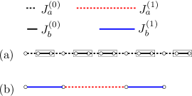
Figure 25: SDRG approach as applied to the spin-$1$ Fibonacci-Heisenberg chain with $L=14$ sites. After sweeping over the effective chain in (b), all spins are eliminated.

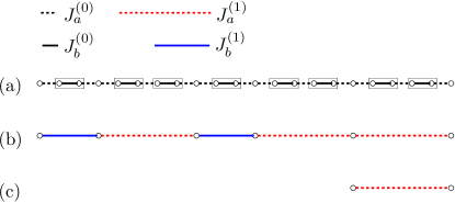
Figure 26: SDRG approach as applied to the spin-$1$ Fibonacci-Heisenberg chain with $L=22$ sites. Sweeping over the effective chain in (b) removes all effective $J_{b}$ bonds, leaving a single effective $J_{a}$ bond, as shown in (c).

An SDRG estimate of the gap for finite open chains can be obtained by stopping the RG scheme at the lowest energy scale for which at least two spins are still active. Figures 25 through 27 illustrate this for chains with $L=14$, $L=22$, and $L=35$ spins. Since we want to obtain estimates to compare with the DMRG results of Sec. IV.5, we need to consider the gap between the ground state, with total spin $S_{T}=0$ or $S_{T}=1$, and the lowest energy level with $S_{T}=2$. For $L=14$ and $L=22$, the ground state is a singlet ($S_{T}=0$), while for $L=35$, with an odd number of spins, the ground state has total spin $S_{T}=1$.

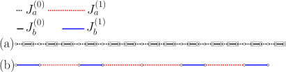
Figure 27: SDRG approach as applied to the spin-$1$ Fibonacci-Heisenberg chain with $L=35$ sites. After sweeping over the effective chain in (b), the central spin remains.

As shown in Fig. 25, for $L=14$ spins, the lowest $S_{T}=2$ energy level corresponds to exciting two pairs of spins to the local $S=1$ states. Thus, the SDRG estimate for this gap is $2J_{b}^{(1)}$, with the effective $J_{b}^{(1)}$ calculated from Eq. (21). For $L=22$, as depicted in Fig.  26, the lowest $S_{T}=2$ excitation comes from a local $S=2$ excitation of a pair of spins connected by an effective $J_{a}^{(1)}$ bond, yielding a gap of $3J_{a}^{(1)}$. Finally, since the ground state for $L=35$ has total spin $S_{T}=1$, the lowest $S_{T}=2$ excitation corresponds to the local excitation of a single spin pair, leading to a gap of $J_{b}^{(1)}$, as shown in Fig. 27. Notice that this explains the nonmonotonic behavior of the gaps with increasing system size, for $r\gtrsim 5$, as observed in Fig. 12.

Estimates of the SDRG gap for larger values of $L$ can be obtained in an analogous fashion.

References

- (1) F. D. M. Haldane, Phys. Rev. Lett. 50, 1153 (1983)
- (2) I. Affleck, J. Phys.: Condens. Matter 1, 3047 (1989)
- (3) I. Affleck, T. Kennedy, E. H. Lieb, and H. Tasaki, Phys. Rev. Lett. 59, 799 (1987)
- (4) M. den Nijs and K. Rommelse, Phys. Rev. B 40, 4709 (Sep 1989)
- (5) S.-K. Ma, C. Dasgupta, and C.-K. Hu, Phys. Rev. Lett. 43, 1434 (1979)
- (6) C. Dasgupta and S.-K. Ma, Phys. Rev. B 22, 1305 (1980)
- (7) C. A. Doty and D. S. Fisher, Phys. Rev. B 45, 2167 (1992)
- (8) D. S. Fisher, Phys. Rev. B 50, 3799 (1994)
- (9) P. Henelius and S. M. Girvin, Phys. Rev. B 57, 11457 (1998)
- (10) N. Laflorencie, H. Rieger, A. W. Sandvik, and P. Henelius, Phys. Rev. B 70, 054430 (2004)
- (11) J. A. Hoyos, A. P. Vieira, N. Laflorencie, and E. Miranda, Phys. Rev. B 76, 174425 (2007)
- (12) K. Damle, Phys. Rev. B 66, 104425 (2002)
- (13) A. Saguia, B. Boechat, and M. A. Continentino, Phys. Rev. Lett. 89, 117202 (2002)
- (14) R. A. Hyman and K. Yang, Phys. Rev. Lett. 78, 1783 (1997)
- (15) R. A. Hyman, Ph.D. thesis, Indiana University (1996)
- (16) C. Monthus, O. Golinelli, and T. Jolicoeur, Phys. Rev. Lett. 79, 3254 (1997)
- (17) C. Monthus, O. Golinelli, and T. Jolicoeur, Phys. Rev. B 58, 805 (1998)
- (18) S. Bergkvist, P. Henelius, and A. Rosengren, Phys. Rev. B 66, 134407 (2002)
- (19) P. Lajkó, E. Carlon, H. Rieger, and F. Iglói, Phys. Rev. B 72, 094205 (2005)
- (20) Y. Nishiyama, Physica A 252, 35 (1998)
- (21) K. Hida, Phys. Rev. Lett. 83, 3297 (1999)
- (22) K. Yang and R. A. Hyman, Phys. Rev. Lett. 84, 2044 (2000)
- (23) S. Todo, K. Kato, and H. Takayama, J. Phys. Soc. Japan 69A, 355 (2000)
- (24) R. B. Griffiths, Phys. Rev. Lett. 23, 17 (1969)
- (25) D. Schechtman, I. Blech, D. Gratias, and J. W. Cahn, Phys. Rev. Lett. 53, 1951 (1984)
- (26) A. P. Vieira, Phys. Rev. Lett. 94, 077201 (2005)
- (27) A. P. Vieira, Phys. Rev. B 71, 134408 (2005)
- (28) F. Iglói and C. Monthus, Phys. Rep. 412, 277 (2005)
- (29) K. Hida, Phys. Rev. B 45, 2207 (1992)
- (30) A. Sandvik and J. Kurkijärvi, Phys. Rev. B 43, 5950 (1991)
- (31) A. Sandvik, J. Phys A. 25, 3667 (1992)
- (32) O. F. Syljuåsen and A. Sandvik, Phys. Rev. E 66, 046701 (2002)
- (33) S. R. White, Phys. Rev. Lett. 69, 2863 (1992)
- (34) I. P. McCulloch, J. Stat. Mech, P10014(2007)
- (35) I. P. McCulloch and M. Gulácsi, Europhys. Lett. 57, 852 (2002)
- (36) We also performed calculations for periodic boundary conditions, but convergence was far more problematic than for open chains.
- (37) Of course, for weak or moderate modulation further-neighbor couplings extend over larger and larger distances, making numerical implementations of the SDRG quite intricate. These cases are not considered here.
- (38) F. J. Oliveira Filho, M. S. Faria, and A. P. Vieira, J. Stat. Mech. 2012, P03007 (2012)
- (39) H. Barghathi, D. Nozadze, and T. Vojta, Phys. Rev. E 89, 012112 (2014)
- (40) See http://physics.uq.edu.au/people/ianmcc/mptoolkit/
- (41) F. Alet, S. Wessel, and M. Troyer, Phys. Rev. E 71, 036706 (Mar 2005)
- (42) A. Albuquerque, F. Alet, P. Corboz, P. Dayal, A. Feiguin, S. Fuchs, L. Gamper, E. Gull, S. Gürtler, A. Honecker, R. Igarashi, M. Körner, A. Kozhevnikov, A. Läuchli, S. Manmana, M. Matsumoto, I. McCulloch, F. Michel, R. Noack, G. P. owski, L. Pollet, T. Pruschke, U. Schollwöck, S. Todo, S. Trebst, M. Troyer, P. Werner, and S. Wessel, J. Magn. Magn. Mater. 310, 1187 (2007), ISSN 0304-8853
- (43) See http://alps.comp-phys.org