A. ALIKHANYAN NATIONAL SCIENCE LABORATORY
YEREVAN PHYSICS INSTITUTE

DEPARTMENT OF THEORETICAL PHYSICS

Geometric Measure of Entanglement and Schmidt Decomposition of Multipartite Systems

Abstract

The thesis includes the original results of our articles  [31, 38, 41, 43, 52, 54, 76]. These results are described in a concise form below.

A method is developed to compute analytically entanglement measures of three-qubit pure states. The methods leans on the theorem stating that entanglement measures of the n-party pure state can be expressed by the (n-1)-party reduced state density operator directly. Owing to this theorem algebraic equations are derived for the geometric measure of entanglement and solved explicitly in the cases of most interest. The solutions give analytic expressions for the geometric entanglement measure in a wide range of three-qubit systems, including the general class of W-type states and states which are symmetric under the permutation of two qubits [38, 41].

The same method is used to find the geometric measure of entanglement of generic three-qubit pure states. Closed-form expressions are presented for the geometric measure of entanglement for three-qubit states that are linear combinations of four orthogonal product states. It turns out that the geometric measure for these states has three different expressions depending on the range of definition in parameter space. Each expression of the measure has its own geometrically meaningful interpretation and thus the Hilbert space of three-qubits consists of three different entangled regions. The states that lie on joint surfaces separating different entangled regions, designated as shared states, have particularly interesting features and are dual quantum channels for the perfect teleportation and superdense coding [43].

A powerful method is developed to compute analytically multipartite entanglement measures. The method uses the duality concept and creates a bijection between highly entangled quantum states and their nearest separable states. The bijection gives explicitly the geometric entanglement measure of arbitrary generalized W states of n qubits and singles out two critical points of entanglement in quantum state parameter space. The first critical value separates symmetric and asymmetric entangled regions of highly entangled states, while the second one separates highly and slightly entangled states [31, 76].

The behavior of the geometric entanglement measure of many-qubit W states is analyzed and an interpolating formula is derived. The importance of the interpolating formula in quantum information is threefold. First, it connects quantities that can be easily estimated in experiments. Second, it is an example of how we compute entanglement of a quantum state with many unknowns. Third, one can prepare the W state with a given entanglement bringing into the position a single quantity [52].

Generalized Schmidt decomposition of pure three-qubit states has four positive and one complex coefficients. In contrast to the bipartite case, they are not arbitrary and the largest Schmidt coefficient restricts severely other coefficients. It is derived a non-strict inequality between three-qubit Schmidt coefficients, where the largest coefficient defines the least upper bound for the three nondiagonal coefficients or, equivalently, the three nondiagonal coefficients together define the greatest lower bound for the largest coefficient. Besides, it is shown the existence of another inequality which should establish an upper bound for the remaining Schmidt coefficient [54].

Introduction

Building quantum information processing devices is a great challenge for scientists and engineers of the third millennium  [2, 3]. Compound quantum systems have potential for many quantum processes, including the following applications: factoring of large composite numbers  [4, 5], quantum cryptography [6, 7], superdense coding [8, 9], quantum teleportation [10, 11] and exponential speedup of quantum computers [12, 13, 14]. These remarkable phenomena have provided a basis for the development of modern quantum information science.

The superior performance of quantum systems in computation and communication applications is rooted in a property of quantum mechanical states called entanglement [15, 16, 17]. Quantum entanglement is a physical resource associated with the peculiar nonclassical correlations that are possible between separated quantum systems. It is a fundamental property of quantum systems and a basic physical resource for quantum information science [18]. In general, any task involving distant parties and using up entangled states as a resource benefits from a better understanding of entanglement. It is increasingly realized that quantum entanglement is at the heart of quantum physics and as such it may be of very broad importance for modern science and future technologies.

Entanglement is usually created by direct interactions between subatomic particles. If two particles are entangled, then there is a correlation between the results of measurements performed on entangled pairs, and this correlation is observed even though the entangled pair may have been separated by arbitrarily large distances. In the multipartite case the entanglement is more complicated concept and to distinguish entangled and unentangled quantum states in this case it is necessary to define product states and separable states.

Consider multipartite systems. The Hilbert space of a such system is the tensor product of the Hilbert spaces of single particles. There is a simple definition of unentangled states in the case of pure states. Indeed, the vector(pure state) belonging to the Hilbert space of the multipartite system is called a product state if it is a tensor product of vectors(pure states) belonging to Hilbert spaces of single particles. In other words, a pure state of a multi-particle system is a product state if and only if all subsystems are pure states. Clearly, there is no correlation between subsystems of product states and they are unentangled states.

Consider now mixed states of a multipartite system. The generalization of the definition of unentangled states to mixed states leans on the local operations and classical communication(LOCC). Local operations and classical communication is a method in quantum information theory where a local operation is performed on part of the system, and where the result of that operation is communicated classically to another part where usually another local operation is performed. Since no quantum interaction occurs within these actions it is natural to assume that no entanglement can be created by LOCC alone, which is to say that LOCC can decrease, but never increases entanglement. Hence, any mixed state that can be obtained from product states via LOCC is unentangled. It is shown, that if a mixed state is a probability distribution over product states, known as separable states, can be created from product states by LOCC alone [19]. Then there are two definitions: first, separable states are unentangled and second, non-separable states are entangled.

One of the most difficult and at the same time fundamental questions in entanglement theory is quantifying entanglement [20, 21, 22]. The basic requirements to an entanglement measures rely on LOCC and local unitary transformations(LU) that is unitary transformations which act on single particles separately. These requirements can be formulated as follows [19]:

• Separable states contain no entanglement.

• All nonseparable states are entangled.

• The entanglement of states does not increase under LOCC operations.

• Entanglement does not change under LU-transformations.

Many entanglement measures have been proposed for the two-particle as well as for the multi-particle case [19]. They are very difficult to compute as their definition contains optimizations over certain quantum states or quantum information protocols. In bipartite case entanglement is relatively well understood, while in multipartite case quantifying entanglement of pure states is a question of vital importance.

The geometric measure of entanglement(GM) is one of the most reliable quantifiers of multipartite entanglement [23, 24, 25, 26]. It measures the distance of a given quantum state from the set of product states and is a decreasing function of the maximal product overlap of the quantum state. The maximal product overlap (MPO) of a quantum pure state is the absolute value of the inner product of the quantum state and its nearest separable state. It(or its square) has several names and we list all of them for the completeness: entanglement eigenvalue [26], injective tensor norm [27], maximal probability of success [29], maximum singular value [30] and maximal product overlap [31].

The geometric measure of entanglement (GM) has the following remarkable properties and applications:

1. It has identified irregularity in channel capacity additivity. Using this measure, one can show that a family of quantities, which were thought to be additive in earlier papers, actually are not [27].

2. It has an operational treatment and quantifies how well a given state serves as an input state to Grover’s search algorithm [28, 29].

3. It has useful connections to other entanglement measures and gives rise to a lower bound on the relative entropy of entanglement [32] and generalized robustness [33].

4. It quantifies the difficulty to distinguish multipartite quantum states by local means [34].

5. It exhibits interesting connections with entanglement witnesses and can be efficiently estimated in experiments [35].

6. It has been used to prove that one dimensional quantum systems tend to be globally separable along renormalization group flows by following a universal scaling law in the correlation length of the system. Owing to this one can understand the physical implication of Zamolodchikov’s c-theorem more deeply [36].

7. It has been used to study quantum phase transitions in spin models [37].

8. It singles out states that can be used as a quantum channel for the perfect teleportation and superdence coding [38].

9. It gives the largest coefficient of the generalized Schmidt decomposition and the corresponding nearest product state uniquely defines the factorisable basis of the decomposition [39].

10. It has been used to derive a single-parameter family of the maximally entangled three-qubit states, where the paradigmatic Greenberger-Horne-Zeilinger and W states emerge as the extreme members in this family of maximally entangled states  [40].

Owing to these features, GM can play an important role in the investigation of different problems related to entanglement. In spite of its usefulness one obstacle to use GM fully in quantum information theories is the that it is difficult to compute it analytically for generic states. The usual maximization method generates a system of nonlinear equations which are unsolvable in general. Thus, it is important to develop a technique for the computation of GM  [41, 42, 43, 44, 45].

For bipartite systems maim problems problems related to entanglement have been solved with the help of the Schmidt decomposition [46, 47]. Therefore its generalization to multipartite states can solve difficult problems related to multipartite entanglement. This generalization for three qubits is done by Acín et al [48], where it is shown that an arbitrary pure state can be written as a linear combination of five product states. Independently, Carteret et al developed a method for such a generalization for pure states of arbitrary multipartite system, where the dimensions of the individual state spaces are finite but otherwise arbitrary [39].

However, for a given quantum state the canonical form is not unique and the same state can have different canonical forms and therefore different sets of such amplitudes. The reason is that the stationarity equations defining stationarity points are nonlinear equations and in general have several solutions of different types. Then the question is which of amplitude sets should be treated as Schmidt coefficients and which ones should be treated as insignificant mathematical solutions. A criterion should exist that can distinguish right Schmidt coefficients from false ones and we need such a criterion. It is unlikely that we can solve problems of three-qubit entanglement without knowledge of what quantities are the relevant entanglement parameters.

The main goals of the thesis are:

 a)

to develop methods that allow us to compute analytically multipartite entanglement measures,

 b)

to derive analytic expressions for the geometric measure of entanglement of multi-particle systems,

 c)

to analyze basic phenomena in quantum information theory using closed form solutions for geometric measure.

 d)

to find inequalities which define a unique Schmidt decomposition for generic multipartite systems

We have developed two powerful methods to compute analytically multipartite entanglement measures.

The first method, hereafter referred to as reduced density method, allows us to compute analytically entanglement measures of three-qubit pure states. The three-qubit system is important in the sense that it is the simplest system which gives a nontrivial effect in the entanglement. Thus, we should understand the general properties of the entanglement in this system as much as possible to go further to more complicated higher-qubit systems. The three-qubit system can be entangled in two inequivalent ways – Greenberger-Horne-Zeilinger (GHZ) [49] and W – and neither form can be transformed into the other with any probability of success [50]. This picture is complete: any fully entangled three-qubit pure state can be obtained from either the GHZ or W state via stochastic local operations and classical communication (SLOCC).

The reduced density method leans on the theorem stating that any reduced (n-1)-qubit state uniquely determines the entanglement of the original n-qubit pure state [51]. This means that two-qubit mixed states can be used to calculate the geometric measure of three-qubit pure states. This idea converts the task effectively into the maximization of the two-qubit mixed state over product states and yields linear eigenvalue equations. Owing to this substantial simplification closed form expressions can be derived for the geometric measure of three-qubit pure states. This is fully addressed in works [38, 43, 41].

The second method, hereafter referred to as duality method, allows us to compute analytically the entanglement measures of highly entangled n-qubit pure states. The main point of the method is the theorem stating that the nearest product state is essentially unique if the quantum state is highly entangled [31]. This makes it possible to map highly entangled state to its nearest product state and quickly obtain its geometric measure of entanglement. More precisely, we construct two bijections. The first one creates a map between highly entangled n-qubit quantum states and n-dimensional unit vectors. The second one does the same between n-dimensional unit vectors and n-part product states. Thus we obtain a double map, or duality, as follows

n-qubit pure states $\leftrightarrow$ n-dimensional spatial vectors $\leftrightarrow$ n-part product states.

The main advantage of the map is that if one knows any of the three vectors, then one instantly finds the other two. Hence we find the geometric measure of entanglement of general multiqubit W states.

The derived answer shows that highly entangled W states have two exceptional points in the parameter space. At the second exceptional point the reduced density operator of a some qubit is a constant multiple of the unit operator and then the maximal product overlap of these states is a constant regardless how many qubits are involved and what are the values of the remaining entanglement parameters. These states are known as shared quantum states and can be used as quantum channels for the perfect teleportation and dense coding.

Next it is shown that W-states have two different entangled regions: the symmetric and asymmetric entangled regions. In the computational basis these regions can be defined as follows. If a W state is in the symmetric region, then the entanglement is a fully symmetric function on the state parameters. Conversely, if a W state is in the asymmetric region, then there is an exceptional parameter such that the entanglement dependence on the exceptional parameter differs dramatically from the dependencies of the remaining parameters. Hence the point of intersection of the symmetric and asymmetric regions is the first exceptional point.

The first exceptional point is important for large-scale W states [52]. It approaches to a fixed point when number of qubits n increases and becomes state-independent(up to 1/n corrections) when $n\gg 1$. As a consequence the entanglement, as well as the maximal product overlap, becomes state-independent too and therefore many-qubit W states have two state-independent exceptional points. The underlying concept is that states whose entanglement parameters differ widely may nevertheless have the same maximal product overlap and this phenomenon should occur at two fixed points. This is an analog of the universality of dynamical systems at critical points. It is an intriguing fact that systems with quite different microscopic parameters may behave equivalently at criticality. Fortunately the renormalization group provides an explanation for the emergence of universality in critical systems [53].

To construct generalized Schmidt decomposition(GSD) for arbitrary systems we apply the variational principle [54]. In order to extend uniquely the Schmidt decomposition to multipartite systems we require that its largest coefficient, as in bipartite case, is the maximal product overlap, otherwise it is an irrelevant solution of stationarity equations. It is clear how do we single out the canonical form whose largest coefficient is the maximal product overlap. We should single out the closest product state of a given quantum state that gives a true maximum for overlap. Of course, we cannot find closest product states of generic three-qubit states because there is no method to solve generic stationarity equation so far. Hence to distinguish the true maximum from other stationary points we require that the second variation of the maximal product overlap is negative everywhere and this condition yields the desired inequality.

The thesis consists of Introduction, six Chapters, Summary and Bibliography.

In Chapter 1 we use the reduced density method to compute analytically the geometric measure of entanglement of GHZ-type and W-type three-qubit pure states [38]. We derive explicit expressions for the maximal product overlaps and closest product states of those states and show that W-type states consist of two different classes. They are: slightly entangled W-states for which MPO is the absolute value of the largest amplitude of the quantum state in the computational basis and highly entangled W-states for which MPO is the circumradius of the triangle whose sides are absolute values of the amplitudes of the quantum state in the same basis.

In Chapter 2 the same method is used to connect the maximal product overlap with the polynomial invariants of three-qubit pure states [41]. It is well known that these states have five polynomial invariants [55], i.e. invariants under LU-transformations. Since entanglement should be invariant under LU-transformations polynomial invariants are real variables of entanglement measures and the relation between MPO and polynomial invariants is independent from the choice of a particular computational basis. Hence we use this relation to classify entangled regions of the Hilbert space as follows: in each region some of polynomial invariants are important and define uniquely MPO while the remaining polynomial invariants are irrelevant. In this way we obtained six different entangled regions for three-qubit pure states.

In Chapter 3 we use the reduced density method to compute analytically the geometric entanglement measure of generic three-qubit pure states which are linear superpositions of GHZ- and W-type states [43]. We give an explicit expression for the geometric measure of entanglement for three-qubit states that are linear combinations of four orthogonal product states. It turns out that the geometric measure for these states has three different expressions depending on the range of definition in parameter space. Each expression of the measure has its own geometrically meaningful interpretation. Such an interpretation allows oneself to take one step toward a complete understanding for the general properties of the entanglement measure. The states that lie on joint surfaces separating different ranges of definition, designated as shared states, are dual quantum channels for the perfect teleportation and superdense coding. The properties of the shared states are fully discussed.

In Chapter 4 we use the duality method to compute analytically the geometric entanglement measure of generic n-qubit W-type states [31]. We have constructed correspondences among W states, n-dimensional unit vectors, and separable pure states. The map reveals two critical values for quantum state parameters. The first critical value separates symmetric and asymmetric entangled regions of highly entangled states, while the second one separates highly and slightly entangled states. The method gives an explicit expressions for the geometric measure when the state allows analytical solutions; otherwise it expresses the entanglement as an implicit function of state parameters.

In Chapter 5 we analyze physical features of entanglement of many-quabit pure states [52]. We show that when $n\gg 1$ the geometric entanglement measure of general n-qubit W-states, except maximally entangled W-states, is a one-variable function and depends only on the Bloch vector with the minimal $z$ component. Hence one can prepare a W state with the required maximal product overlap by altering the Bloch vector of a single qubit. Next we compute analytically the geometric measure of large-scale W states by describing these systems in terms of very few parameters. The final formula relates two quantities, namely the maximal product overlap and the Bloch vector, that can be easily estimated in experiments.

In Chapter 6 we derive a non-strict inequality between three-qubit Schmidt coefficients, where the largest coefficient defines the least upper bound for the three nondiagonal coefficients or, equivalently, the three nondiagonal coefficients together define the greatest lower bound for the largest coefficient. The main role of the inequality is to separate out three-qubit Schmidt coefficients from the set of four positive and one complex numbers. Besides, it is shown the existence of another inequality which should establish an upper bound for the remaining Schmidt coefficient.

In Summary we give the main points of our results and conclusions.

In Bibliography we list our references in order of appearance.

Chapter 1 Analytic Expressions for Geometric Measure of Three Qubit States

In this chapter we compute analytically the geometric measure of entanglement of three-qubit pure states [38].

The entanglement of bipartite systems is well-understood [20, 21, 22, 56], while the entanglement of multipartite systems offers a real challenge to physicists. The main point which makes difficult to understand the entanglement for the multi-qubit systems is mainly due to the fact that the analytic expressions for the various entanglement measures is extremely hard to derive.

We consider pure three qubit systems [48, 57, 58, 59, 60], although the entanglement of mixed states attracts a considerable attention. Only very few analytical results for tripartite entanglement have been obtained so far and we need more light on the subject.

Recently the idea was suggested that nonlinear eigenproblem can be reduced to the linear eigenproblem for the case of three qubit pure states [51]. The idea is based on theorem stating that any reduced $(n-1)$-qubit state uniquely determines the geometric measure of the original $n$-qubit pure state. This means that two qubit mixed states can be used to calculate the geometric measure of three qubit pure states and this will be fully addressed in this work.

The method gives two algebraic equations of degree six defining the geometric measure of entanglement. Thus the difficult problem of geometric measure calculation is reduced to the algebraic equation root finding. Equations contain valuable information, are good bases for the numerical calculations and may test numerical calculations based on other numerical techniques [61].

Furthermore, the method allows to find the nearest separable states for three qubit states of most interest and get analytic expressions for their geometric measures. It turn out that highly entangled states have their own feature. Each highly entangled state has a vicinity with no product state and all nearest product states are on the boundary of the vicinity and form an one-parametric set.

This chapter is organized as follows. In Section 1.1 we define the geometric measure of entanglement and derive stationarity equations. In Section 1.2 we derive algebraic equations in the case of pure three qubit states and give general solutions. In Section 1.3 we examine W-type states and deduce analytic expression for their geometric measures. States symmetric under permutation of two qubits are considered in Section 1.4, where the overlap of the state functions with the product states are maximized directly. In last Section 1.5 we make concluding remarks.

1.1 Geometric measure of entanglement

We start by developing a general formulation, appropriate for multipartite systems comprising n parts, in which each part has its distinct Hilbert space. Let $|\psi\rangle$ be a pure state of an $n$-party system ${\cal H}={\cal H}_{1}\otimes{\cal H}_{2}\otimes\cdots\otimes{\cal H}_{n}$ , where the dimensions of the individual state spaces ${\cal H}_{k}$ are finite but otherwise arbitrary. Denote by $|q_{1}q_{2}...q_{n}\rangle$ product states which are defined as the tensor products

$$|q_{1}q_{2}...q_{n}\rangle\equiv|q_{1}\rangle\otimes|q_{2}\rangle\otimes\cdots\otimes|q_{n}\rangle,$$

where $|q_{k}\rangle\in{\cal H}_{k},k=1,2,...,n$.

The geometric measure of entanglement $E_{g}$ for an $n$-part pure state $\psi$ is defined as $E_{g}(\psi)=-\ln\Lambda_{\max}^{2}(\psi)$, where the maximal product overlap $\Lambda_{max}(\psi)$ is given by [26]

$$\Lambda_{max}=\max_{q_{1},q_{2},...,q_{n}}|\left\langle\psi|q_{1}q_{2}...q_{n}\right\rangle|,$$ (1.1)

where the normalization condition $\left\langle q_{k}|q_{k}\right\rangle=1(k=1,2,...,n)$ is understood and the maximization is performed over all product states.

The nearest product state is a stationary point for the overlap with $|\psi\rangle$, so the states $|q_{k}\rangle$ satisfy the nonlinear eigenvalue equations

$$\langle q_{1}q_{2}\cdots\widehat{q_{k}}\cdots q_{n}|\psi\rangle=\Lambda_{k}|q_{k}\rangle;\;k=1,2,\cdots,n,$$ (1.2)

where the caret means exclusion and eigenvalues $\Lambda_{k}$ are associated with the Lagrange multipliers enforcing constraints $\left\langle q_{k}|q_{k}\right\rangle=1(k=1,2,...,n)$.

Since phases of local states $|q_{k}\rangle$ are irrelevant one can choose them such that $\Lambda_{k}$’s are all positive. On the other hand $|\Lambda_{k}|=\Lambda_{max}$ and therefore the stationarity equations can be rewritten as

$$\langle q_{1}q_{2}\cdots\widehat{q_{k}}\cdots q_{n}|\psi\rangle=\Lambda_{max}|q_{k}\rangle;\;k=1,2,\cdots,n.$$ (1.3)

This is a system of nonlinear equations and its maximal eigenvalue and corresponding eigenvector are the maximal product overlap and the nearest product state of a given pure states $|\psi\rangle$, respectively.

The extension of the geometric measure of entanglement to mixed states can be made via the use of the convex roof (or hull ) construction, as it is done for the entanglement of formation [21]. We omit it since mixed states are not considered in this thesis.

1.2 Algebraic equations.

Consider now three qubits A,B,C with state function $|\psi\rangle$. The entanglement eigenvalue $\Lambda_{max}(\psi)$ is given by

$$\Lambda_{max}=\max_{q^{1}q^{2}q^{3}}|\langle q^{1}q^{2}q^{3}|\psi\rangle|$$ (1.4)

and the maximization runs over all normalized complete product states $|q^{1}\rangle\otimes|q^{2}\rangle\otimes|q^{3}\rangle$. Superscripts label single qubit states and spin indices are omitted for simplicity. Since in the following we will use density matrices rather than state functions, our first aim is to rewrite Eq.(1.4) in terms of density matrices. Let us denote by $\rho^{ABC}=|\psi\rangle\langle\psi|$ the density matrix of the three-qubit state and by $\varrho^{k}=|q^{k}\rangle\langle q^{k}|$ the density matrices of the single qubit states. The equation for the square of the entanglement eigenvalue takes the form

$$\Lambda_{\max}^{2}(\psi)=\max_{\varrho^{1}\varrho^{2}\varrho^{3}}\mathrm{tr}\left(\rho^{ABC}\varrho^{1}\otimes\varrho^{2}\otimes\varrho^{3}\right).$$ (1.5)

An important equality

$$\max_{\varrho^{3}}\mathrm{tr}(\rho^{ABC}\varrho^{1}\otimes\varrho^{2}\otimes\varrho^{3})=\mathrm{tr}(\rho^{ABC}\varrho^{1}\otimes\varrho^{2}\otimes{\textsl{1\!\!1}}^{3})$$ (1.6)

was derived in [51] where 1​​1 is a unit matrix. It has a clear meaning. The matrix $\mathrm{tr}(\rho^{ABC}\varrho^{1}\otimes\varrho^{2})$ is $2\otimes 2$ hermitian matrix and has two eigenvalues. One of eigenvalues is always zero and another is always positive and therefore the maximization of the matrix simply takes the nonzero eigenvalue. Note that its minimization gives zero as the minimization takes the zero eigenvalue.

We use Eq.(1.6) to reexpress the entanglement eigenvalue by reduced density matrix $\rho^{AB}$ of qubits A and B in a form

$$\Lambda_{\max}^{2}(\psi)=\max_{\varrho^{1}\varrho^{2}}\mathrm{tr}\left(\rho^{AB}\varrho^{1}\otimes\varrho^{2}\right).$$ (1.7)

We denote by ${\bm{s}}_{1}$ and ${\bm{s}}_{2}$ the unit Bloch vectors of the density matrices $\varrho^{1}$ and $\varrho^{2}$ respectively and adopt the usual summation convention on repeated indices $i$ and $j$. Then

$$\Lambda_{\max}^{2}=\frac{1}{4}\max_{s_{1}^{2}=s_{2}^{2}=1}\left(1+{\bm{s}}_{1}\cdot{\bm{r}}_{1}+{\bm{s}}_{2}\cdot{\bm{r}}_{2}+g_{ij}\,s_{1i}s_{2j}\right),$$ (1.8)

where

$${\bm{r}}_{1}=\mathrm{tr}(\rho^{A}{\bm{\sigma}}),\,\,{\bm{r}}_{2}=\mathrm{tr}(\rho^{B}{\bm{\sigma}}),\,\,g_{ij}=\mathrm{tr}(\rho^{AB}\sigma_{i}\otimes\sigma_{j})$$ (1.9)

and $\sigma_{i}$’s are Pauli matrices. The matrix $g_{ij}$ is not necessarily to be symmetric but must has only real entries. The maximization gives a pair of equations

$${\bm{r}}_{1}+g{\bm{s}}_{2}=\lambda_{1}{\bm{s}}_{1},\quad{\bm{r}}_{2}+g^{T}{\bm{s}}_{1}=\lambda_{2}{\bm{s}}_{2},$$ (1.10)

where Lagrange multipliers $\lambda_{1}$ and $\lambda_{2}$ are enforcing unit nature of the Bloch vectors. The solution of Eq.(1.10) is

$${\bm{s}}_{1}=\left(\lambda_{1}\lambda_{2}{\textsl{1\!\!1}}-g\,g^{T}\right)^{-1}\left(\lambda_{2}{\bm{r}}_{1}+g\,{\bm{r}}_{2}\right),$$ (1.11a)

$${\bm{s}}_{2}=\left(\lambda_{1}\lambda_{2}{\textsl{1\!\!1}}-g^{T}g\right)^{-1}\left(\lambda_{1}{\bm{r}}_{2}+g^{T}{\bm{r}}_{1}\right).$$ (1.11b)

Now, the only unknowns are Lagrange multipliers, which should be determined by equations

$$|{\bm{s}}_{1}|^{2}=1,\quad|{\bm{s}}_{2}|^{2}=1.$$ (1.12)

In general, Eq.(1.12) give two algebraic equations of degree six. However, the solution (1.11) is valid if Eq.(1.10) supports a unique solution and this is by no means always the case. If the solution of Eq.(1.10) contains a free parameter, then $\det(\lambda_{1}\lambda_{2}{\textsl{1\!\!1}}-gg^{T})=0$ and, as a result, Eq.(1.11) cannot not applicable. The example presented in Section III will demonstrate this situation.

In order to test Eq.(1.11) let us consider an arbitrary superposition of W

$$|W\rangle=\frac{1}{\sqrt{3}}\left(|100\rangle+|010\rangle+|001\rangle\right)$$ (1.13)

and flipped W

$$|\widetilde{W}\rangle=\frac{1}{\sqrt{3}}\left(|011\rangle+|101\rangle+|110\rangle\right)$$ (1.14)

states, i.e. the state

$$|\psi\rangle=\cos\theta|W\rangle+\sin\theta|\widetilde{W}\rangle.$$ (1.15)

Straightforward calculation yields

$${\bm{r}}_{1}={\bm{r}}_{2}=\frac{1}{3}\left(2\sin 2\theta{\bm{i}}+\cos 2\theta{\bm{n}}\right),$$ (1.16a)

$$g=\frac{1}{3}\begin{pmatrix}2&0&0\\ 0&2&0\\ 0&0&\!\!-1\end{pmatrix},$$ (1.16b)

where unit vectors ${\bm{i}}$ and ${\bm{n}}$ are aligned with the axes $x$ and $z$, respectively. Both vectors ${\bm{i}}$ and ${\bm{n}}$ are eigenvectors of matrices $g$ and $g^{T}$. Therefore ${\bm{s}}_{1}$ and ${\bm{s}}_{2}$ are linear combinations of ${\bm{i}}$ and ${\bm{n}}$. Also from ${\bm{r}}_{1}={\bm{r}}_{2}$ and $g=g^{T}$ it follows that ${\bm{s}}_{1}={\bm{s}}_{2}$ and $\lambda_{1}=\lambda_{2}$. Then Eq.(1.11) for general solution give

$${\bm{s}}_{1}={\bm{s}}_{2}=\sin 2\varphi\,{\bm{i}}+\cos 2\varphi\,{\bm{n}}$$ (1.17)

where

$$\sin 2\varphi=\frac{2\sin 2\theta}{3\lambda-2},\quad\cos 2\varphi=\frac{\cos 2\theta}{3\lambda+1}.$$ (1.18)

The elimination of the Lagrange multiplier $\lambda$ from Eq.(1.18) gives

$$3\sin 2\varphi\cos 2\varphi=\cos 2\theta\sin 2\varphi-2\sin 2\theta\cos 2\varphi.$$ (1.19)

Let us denote by $t=\tan\varphi$. After the separation of the irrelevant root $t=-\tan\theta$, Eq.(1.19) takes the form

$$\sin\theta\,t^{3}+2\cos\theta\,t^{2}-2\sin\theta\,t-\cos\theta=0.$$ (1.20)

This equation exactly coincides with that derived in [26]. Since a detailed analysis was given in Ref.[26], we do not want to repeat the same calculation here. Instead we would like to consider the three-qubit states that allow the analytic expressions for the geometric entanglement measure by making use of Eq.(1.10).

1.3 W-type states.

Consider W-type state

$$|\psi\rangle=a|100\rangle+b|010\rangle+c|001\rangle,\quad a^{2}+b^{2}+c^{2}=1.$$ (1.21)

Without loss of generality we consider only the case of positive parameters $a,b,c$. Direct calculation yields

$${\bm{r}}_{1}=r_{1}\,{\bm{n}},\quad{\bm{r}}_{2}=r_{2}\,{\bm{n}},\quad g=\begin{pmatrix}\omega&0&0\\ 0&\omega&0\\ 0&0&-r_{3}\end{pmatrix},$$ (1.22)

where

$$r_{1}=b^{2}+c^{2}-a^{2},\,r_{2}=a^{2}+c^{2}-b^{2},\,r_{3}=a^{2}+b^{2}-c^{2}$$ (1.23)

and $\omega=2ab$. The unit vector ${\bm{n}}$ is aligned with the axis $z$. Any vector perpendicular to ${\bm{n}}$ is an eigenvector of $g$ with eigenvalue $\omega$. Then from Eq.(1.10) it follows that the components of vectors ${\bm{s}}_{1}$ and ${\bm{s}}_{2}$ perpendicular to ${\bm{n}}$ are collinear. We denote by ${\bm{m}}$ the unit vector along that direction and parameterize vectors ${\bm{s}}_{1}$ and ${\bm{s}}_{2}$ as follows

$${\bm{s}}_{1}=\cos\alpha\,{\bm{n}}+\sin\alpha\,{\bm{m}},\quad{\bm{s}}_{2}=\cos\beta\,{\bm{n}}+\sin\beta\,{\bm{m}}.$$ (1.24)

Then Eq.(1.10) reduces to the following four equations

$$r_{1}-r_{3}\cos\beta=\lambda_{1}\cos\alpha,\quad r_{2}-r_{3}\cos\alpha=\lambda_{2}\cos\beta,$$ (1.25a)

$$\omega\sin\beta=\lambda_{1}\sin\alpha,\quad\omega\sin\alpha=\lambda_{2}\sin\beta,$$ (1.25b)

which are used to solve the four unknown constants $\lambda_{1},\lambda_{2},\alpha$ and $\beta$. Eq.(1.25b) impose either

$$\lambda_{1}\lambda_{2}-\omega^{2}=0$$ (1.26)

or

$$\sin\alpha\sin\beta=0.$$ (1.27)

First consider the case $r_{1}>0,r_{2}>0,r_{3}>0$ and coefficients $a,b,c$ form an acute triangle. Eq.(1.27) does not give a true maximum and this can be understood as follows. If both vectors ${\bm{s}}_{1}$ and ${\bm{s}}_{2}$ are aligned with the axis $z$, then the last term in Eq.(1.8) is negative. If vectors ${\bm{s}}_{1}$ and ${\bm{s}}_{2}$ are antiparallel, then one of scalar products in Eq.(1.8) is negative. In this reason $\Lambda_{\max}^{2}$ cannot be maximal. Then Eq.(1.26) gives true maximum and we have to choose positive values for $\lambda_{1}$ and $\lambda_{2}$ to get maximum.

First we use Eq.(1.25a) to connect the angles $\alpha$ and $\beta$ with the Lagrange multipliers $\lambda_{1}$ and $\lambda_{2}$

$$\cos\alpha=\frac{\lambda_{2}r_{1}-r_{2}r_{3}}{\omega^{2}-r_{3}^{2}},\quad\cos\beta=\frac{\lambda_{1}r_{2}-r_{1}r_{3}}{\omega^{2}-r_{3}^{2}}.$$ (1.28)

Then Eq.(1.25b) and (1.26) give the following expressions for Lagrange multipliers $\lambda_{1}$ and $\lambda_{2}$

$$\lambda_{1}=\omega\left(\frac{\omega^{2}+r_{1}^{2}-r_{3}^{2}}{\omega^{2}+r_{2}^{2}-r_{3}^{2}}\right)^{1/2},$$ (1.29a)

$$\lambda_{2}=\omega\left(\frac{\omega^{2}+r_{2}^{2}-r_{3}^{2}}{\omega^{2}+r_{1}^{2}-r_{3}^{2}}\right)^{1/2}.$$ (1.29b)

Eq.(1.10) allows to write a shorter expression for the entanglement eigenvalue

$$\Lambda_{\max}^{2}=\frac{1}{4}\left(1+\lambda_{2}+r_{1}\cos\alpha\right).$$ (1.30)

Now we insert the values of $\lambda_{2}$ and $\cos\alpha$ into Eq.(1.30) and obtain

$$4\Lambda_{\max}^{2}=1+\frac{\omega\sqrt{(\omega^{2}+r_{1}^{2}-r_{3}^{2})(\omega^{2}+r_{2}^{2}-r_{3}^{2})}-r_{1}r_{2}r_{3}}{\omega^{2}-r_{3}^{2}}.$$ (1.31)

The denominator in above expression is multiple of the area $S$ of the triangle $a,b,c$

$$\omega^{2}-r_{3}^{2}=16S^{2}.$$ (1.32)

A little algebra yields for the numerator

$$\omega\sqrt{(\omega^{2}+r_{1}^{2}-r_{3}^{2})+(\omega^{2}+r_{2}^{2}-r_{3}^{2})}-r_{1}r_{2}r_{3}$$

$$\hskip 8.5359pt=16\,a^{2}b^{2}c^{2}-\omega^{2}+r_{3}^{2}.$$

Combining together the numerator and denominator, we obtain the final expression for the entanglement eigenvalue

$$\Lambda_{\max}^{2}=4R^{2},$$ (1.34)

where $R$ is the circumradius of the triangle $a,b,c$. Entanglement value is minimal when triangle is regular, i.e. for W-state and $\Lambda_{\max}^{2}(W)=4/9$ [62].

Now consider the case $r_{3}<0$. Since $r_{3}+r_{1}=2b^{2}\geq 0$, we have $r_{1}>0$ and similarly $r_{2}>0$. Eq.(1.27) gives true maximum in this case and both vectors are aligned with the axis $z$

$${\bm{s}}_{1}={\bm{s}}_{2}={\bm{n}}$$ (1.35)

resulting in $\Lambda_{\max}^{2}=c^{2}$. In view of symmetry

$$\Lambda_{\max}^{2}=\max(a^{2},b^{2},c^{2}),\quad\max(a^{2},b^{2},c^{2})>\frac{1}{2}.$$ (1.36)

Since the matrix $g$ and vectors ${\bm{r}}_{1}$ and ${\bm{r}}_{2}$ are invariant under rotations around axis $z$ the same properties must have Bloch vectors ${\bm{s}}_{1}$ and ${\bm{s}}_{2}$. There are two possibilities:

i)Bloch vectors are unique and aligned with the axis $z$. The solution given by Eq.(1.35) corresponds to this situation and the resulting entanglement eigenvalue Eq.(1.36) satisfies the inequality

$$\frac{1}{2}<\Lambda_{\max}^{2}\leq 1.$$ (1.37)

ii)Bloch vectors have nonzero components in $xy$ plane and the solution is not unique. Eq.(1.24) corresponds to this situation and contains a free parameter. The free parameter is the angle defining the direction of the vector ${\bm{m}}$ in the $xy$ plane. Then Eq.(1.34) gives the entanglement eigenvalue in highly entangled region

$$\frac{4}{9}\leq\Lambda_{\max}^{2}<\frac{1}{2}.$$ (1.38)

Eq.(1.34) and (1.36) have joint curves when parameters $a,b,c$ form a right triangle and give $\Lambda_{\max}^{2}=1/2$. The GHZ states have same entanglement value and it seems to imply something interesting. GHZ state can be used for teleportation and superdense coding, but W-state cannot be. However, the W-type state with right triangle coefficients can be used for teleportation and superdense coding [63]. In other words, both type of states can be applied provided they have the required entanglement eigenvalue $\Lambda_{\max}^{2}=1/2$.

1.4 Symmetric States.

Now let us consider the state which is symmetric under permutation of qubits A and B and contains three real independent parameters

$$|\psi\rangle=a|000\rangle+b|111\rangle+c|001\rangle+d|110\rangle,$$ (1.39)

where $a^{2}+b^{2}+c^{2}+d^{2}=1$. According to Generalized Schmidt Decomposition [48] the states with different sets of parameters are local-unitary(LU) inequivalent. The relevant quantities are

$${\bm{r}}_{1}={\bm{r}}_{2}=r\,{\bm{n}},\quad g=\begin{pmatrix}\omega&0&0\\ 0&-\omega&0\\ 0&0&1\end{pmatrix},$$ (1.40)

where

$$r=a^{2}+c^{2}-b^{2}-d^{2},\quad\omega=2ad+2bc$$ (1.41)

and the unit vector ${\bm{n}}$ again is aligned with the axis $z$.

All three terms in the l.h.s. of Eq.(1.8) are bounded above:

• ${\bm{s}}_{1}\cdot{\bm{r}}_{1}\leq|r|$,

• ${\bm{s}}_{2}\cdot{\bm{r}}_{2}\leq|r|$,

• and owing to inequality $|\omega|\leq 1,\,g_{ij}\,s_{1i}s_{2j}\leq 1$.

Quite surprisingly all upper limits are reached simultaneously at

$${\bm{s}}_{1}={\bm{s}}_{2}={\rm Sign}(r){\bm{n}},$$ (1.42)

which results in

$$\Lambda_{\max}^{2}=\frac{1}{2}\left(1+|r|\right).$$ (1.43)

This expression has a clear meaning. To understand it we parameterize the state as

$$|\psi\rangle=k_{1}|00q_{1}\rangle+k_{2}|11q_{2}\rangle,$$ (1.44)

where $q_{1}$ and $q_{2}$ are arbitrary single normalized qubit states and positive parameters $k_{1}$ and $k_{2}$ satisfy $k_{1}^{2}+k_{2}^{2}=1$. Then

$$\Lambda_{\max}^{2}=\max(k_{1}^{2},k_{2}^{2}),$$ (1.45)

i.e. the maximization takes a larger coefficient in Eq.(1.44). In bipartite case the maximization takes the largest coefficient in Schmidt decomposition [29, 64] and in this sense Eq.(1.44) effectively takes the place of Schmidt decomposition. When $|q_{1}\rangle=|0\rangle$ and $|q_{2}\rangle=|1\rangle$, Eq.(1.45) gives the known answer for generalized GHZ state [26, 62].

The entanglement eigenvalue is minimal $\Lambda_{\max}^{2}=1/2$ on condition that $k_{1}=k_{2}$. These states can be described as follows

$$|\psi\rangle=|00q_{1}\rangle+|11q_{2}\rangle$$ (1.46)

where $q_{1}$ and $q_{2}$ are arbitrary single qubit normalized states. The entanglement eigenvalue is constant $\Lambda_{\max}^{2}=1/2$ and does not depend on single qubit state parameters. Hence one may expect that all these states can be applied for teleportation and superdense coding. It would be interesting to check whether this assumption is correct or not.

It turns out that GHZ state is not a unique state and is one of two-parametric LU inequivalent states that have $\Lambda_{\max}^{2}=1/2$. On the other hand W-state is unique up to LU transformations and the low bound $\Lambda_{\max}^{2}=4/9$ is reached if and only if $a=b=c$. However, one cannot make such conclusions in general. Five real parameters are necessary to parameterize the set of inequivalent three qubit pure states [48]. And there is no explicit argument that W-state is not just one of LU inequivalent states that have $\Lambda_{\max}^{2}=4/9$.

1.5 Summary.

We have derived algebraic equations defining geometric measure of three qubit pure states. These equations have a degree higher than four and explicit solutions for general cases cannot be derived analytically. However, the explicit expressions are not important. Remember that explicit expressions for the algebraic equations of degree three and four have a limited practical significance but the equations itself are more important. This is especially true for equations of higher degree; main results can be derived from the equations rather than from the expressions of their roots.

Eq.(1.10) give the nearest separable state directly and this separable states have useful applications. In order to construct an entanglement witness, for example, the crucial point lies in finding the nearest separable state [65]. This will be especially interesting for highly entangled states that have a whole set of nearest separable states and allow to construct a set of entanglement witnesses.

The expression in r.h.s. of Eq.(1.8) can be maximized directly for various three qubit states. Although it is very hard to solve the higher-degree equation, it turns out that the wide range of the three-qubit states have a symmetry and this symmetry reduces the equations of degree six to the quadratic equations. In this reason Eq.(1.8) can be used to derive the analytic expressions of the various entanglement measures for the three-qubit states. Also Eq.(1.8) can be a starting point to explore the numerical computation of the entanglement measures for the higher-qubit systems.

Chapter 2 Three-Qubit Groverian Measure

In this chapter we connect the geometric entanglement measure with polynomial invariants in the case of three-quibt pure states [41].

About decade ago the axioms which entanglement measures should satisfy were studied [24]. The most important property for measure is monotonicity under local operation and classical communication(LOCC) [66]. Following the axioms, many entanglement measures were constructed such as relative entropy[67], entanglement of distillation[22] and formation[20, 21, 68, 69], geometric measure[23, 25, 26, 70], Schmidt measure[71] and Groverian measure[29]. Entanglement measures are used in various branches of quantum mechanics. Especially, recently, they are used to try to understand Zamolodchikov’s c-theorem[72] more profoundly. It may be an important application of the quantum information techniques to understand the effect of renormalization group in field theories[36].

The purpose of this paper is to compute the Groverian measure for various three-qubit quantum states. The Groverian measure $G(\psi)$ for three-qubit state $|\psi\rangle$ is defined by $G(\psi)\equiv\sqrt{1-P_{max}}$ where

$$P_{max}=\Lambda_{\max}^{2}$$ (2.1)

Thus $P_{max}$ can be interpreted as a maximal overlap between the given state $|\psi\rangle$ and product states. Groverian measure is an operational treatment of a geometric measure. Thus, if one can compute $G(\psi)$, one can also compute the geometric measure of pure state by $G^{2}(\psi)$. Sometimes it is more convenient to re-express Eq.(2.1) in terms of the density matrix $\rho=|\psi\rangle\langle\psi|$. This can be easily accomplished by an expression

$$P_{max}=\max_{R^{1},R^{2},R^{3}}\mbox{Tr}\left[\rho R^{1}\otimes R^{2}\otimes R^{3}\right]$$ (2.2)

where $R^{i}\equiv|q_{i}\rangle\langle q_{i}|$ density matrix for the product state. Eq.(2.1) and Eq.(2.2) manifestly show that $P_{max}$ and $G(\psi)$ are local-unitary(LU) invariant quantities. Since it is well-known that three-qubit system has five independent LU-invariants[48, 55, 58, 73], say $J_{i}(i=1,\cdots,5)$, we would like to focus on the relation of the Groverian measures to LU-invariants $J_{i}$’s in this paper.

This chapter is organized as follows.

In Section 2.1 we review simple case, i.e. two-qubit system. Using Bloch form of the density matrix it is shown in this section that two-qubit system has only one independent LU-invariant quantity, say $J$. It is also shown that Groverian measure and $P_{max}$ for arbitrary two-qubit states can be expressed solely in terms of $J$.

In Section 2.2 we have discussed how to derive LU-invariants in higher-qubit systems. In fact, we have derived many LU-invariant quantities using Bloch form of the density matrix in three-qubit system. It is shown that all LU-invariants derived can be expressed in terms of $J_{i}$’s discussed in Ref.[48]. Recently, it was shown in Ref.[51] that $P_{max}$ for $n$-qubit state can be computed from $(n-1)$-qubit reduced mixed state. This theorem was used in Ref.[38] and Ref.[43] to compute analytically the geometric measures for various three-qubit states. In this section we have discussed the physical reason why this theorem is possible from the aspect of LU-invariance.

In Section 2.3 we have computed the Groverian measures for various types of the three-qubit system. The five types we discussed in this section were originally developed in Ref.[48] for the classification of the three-qubit states. It has been shown that the Groverian measures for type 1, type 2, and type 3 can be analytically computed. We have expressed all analytical results in terms of LU-invariants $J_{i}$’s. For type 4 and type 5 the analytical computation seems to be highly nontrivial and may need separate publications. Thus the analytical calculation for these types is not presented in this paper. The results of this section are summarized in Table I.

In Section 2.4 we have discussed the modified W-like state, which has three-independent real parameters. In fact, this state cannot be categorized in the five types discussed in Section 2.3. The analytic expressions of the Groverian measure for this state was computed recently in Ref.[43]. It was shown that the measure has three different expressions depending on the domains of the parameter space. It turned out that each expression has its own geometrical meaning. In this section we have re-expressed all expressions of the Groverian measure in terms of LU-invariants.

In Section 2.5 brief conclusion is given.

2.1 Two Qubit: Simple Case

In this section we consider $P_{max}$ for the two-qubit system. The Groverian measure for two-qubit system is already well-known[62]. However, we revisit this issue here to explore how the measure is expressed in terms of the LU-invariant quantities. The Schmidt decomposition[46, 47] makes the most general expression of the two-qubit state vector to be simple form

$$|\psi\rangle=\lambda_{0}|00\rangle+\lambda_{1}|11\rangle$$ (2.3)

with $\lambda_{0},\lambda_{1}\geq 0$ and $\lambda_{0}^{2}+\lambda_{1}^{2}=1$. The density matrix for $|\psi\rangle$ can be expressed in the Bloch form as following:

$$\rho=|\psi\rangle\langle\psi|=\frac{1}{4}\left[{\textsl{1\!\!1}}\otimes{\textsl{1\!\!1}}+v_{1\alpha}\sigma_{\alpha}\otimes{\textsl{1\!\!1}}+v_{2\alpha}{\textsl{1\!\!1}}\otimes\sigma_{\alpha}+g_{\alpha\beta}\sigma_{\alpha}\otimes\sigma_{\beta}\right],$$ (2.4)

where

$$\vec{v}_{1}=\vec{v}_{2}=\left(\begin{array}[]{c}0\\ 0\\ \lambda_{0}^{2}-\lambda_{1}^{2}\end{array}\right),\hskip 28.45274ptg_{\alpha\beta}=\left(\begin{array}[]{ccc}2\lambda_{0}\lambda_{1}&0&0\\ 0&-2\lambda_{0}\lambda_{1}&0\\ 0&0&1\end{array}\right).$$ (2.11)

In order to discuss the LU transformation we consider first the quantity $U\sigma_{\alpha}U^{\dagger}$ where $U$ is $2\times 2$ unitary matrix. With direct calculation one can prove easily

$$U\sigma_{\alpha}U^{\dagger}={\cal O}_{\alpha\beta}\sigma_{\beta},$$ (2.12)

where the explicit expression of ${\cal O}_{\alpha\beta}$ is given in appendix A. Since ${\cal O}_{\alpha\beta}$ is a real matrix satisfying ${\cal O}{\cal O}^{T}={\cal O}^{T}{\cal O}={\textsl{1\!\!1}}$, it is an element of the rotation group O(3). Therefore, Eq.(2.12) implies that the LU-invariants in the density matrix (2.4) are $|\vec{v}_{1}|$, $|\vec{v}_{2}|$, $\mbox{Tr}[gg^{T}]$ etc.

All LU-invariant quantities can be written in terms of one quantity, say $J\equiv\lambda_{0}^{2}\lambda_{1}^{2}$. In fact, $J$ can be expressed in terms of two-qubit concurrence[21] ${\cal C}$ by ${\cal C}^{2}/4$. Then it is easy to show

$$|\vec{v}_{1}|^{2}=|\vec{v}_{2}|^{2}=1-4J,$$ (2.13)

$$g_{\alpha\beta}g_{\alpha\beta}=1+8J.$$

It is well-known that $P_{max}$ is simply square of larger Schmidt number in two-qubit case

$$P_{max}=\mbox{max}\left(\lambda_{0}^{2},\lambda_{1}^{2}\right).$$ (2.14)

It can be re-expressed in terms of reduced density operators

$$P_{max}=\frac{1}{2}\left[1+\sqrt{1-4\mbox{det}\rho^{A}}\right],$$ (2.15)

where $\rho^{A}=\mbox{Tr}_{B}\rho=(1+v_{1\alpha}\sigma_{\alpha})/2$. Since $P_{max}$ is invariant under LU-transformation, it should be expressed in terms of LU-invariant quantities. In fact, $P_{max}$ in Eq.(2.15) can be re-written as

$$P_{max}=\frac{1}{2}\left[1+\sqrt{1-4J}\right].$$ (2.16)

Eq.(2.16) implies that $P_{max}$ is manifestly LU-invariant.

2.2 Local Unitary Invariants

The Bloch representation of the $3$-qubit density matrix can be written in the form

$$\rho = \frac{1}{8}\Bigg{[}{\textsl{1\!\!1}}\otimes{\textsl{1\!\!1}}\otimes{\textsl{1\!\!1}}+v_{1\alpha}\sigma_{\alpha}\otimes{\textsl{1\!\!1}}\otimes{\textsl{1\!\!1}}+v_{2\alpha}{\textsl{1\!\!1}}\otimes\sigma_{\alpha}\otimes{\textsl{1\!\!1}}+v_{3\alpha}{\textsl{1\!\!1}}\otimes{\textsl{1\!\!1}}\otimes\sigma_{\alpha}$$ (2.17)

$$+h^{(1)}_{\alpha\beta}{\textsl{1\!\!1}}\otimes\sigma_{\alpha}\otimes\sigma_{\beta}+h^{(2)}_{\alpha\beta}\sigma_{\alpha}\otimes{\textsl{1\!\!1}}\otimes\sigma_{\beta}+h^{(3)}_{\alpha\beta}\sigma_{\alpha}\otimes\sigma_{\beta}\otimes{\textsl{1\!\!1}}$$

$$+g_{\alpha\beta\gamma}\sigma_{\alpha}\otimes\sigma_{\beta}\otimes\sigma_{\gamma}\Bigg{]},\vspace{1cm}$$

where $\sigma_{\alpha}$ is Pauli matrix. According to Eq.(2.12) and appendix A it is easy to show that the LU-invariants in the density matrix (2.17) are $|\vec{v}_{1}|$, $|\vec{v}_{2}|$, $|\vec{v}_{3}|$, $\mbox{Tr}[h^{(1)}h^{(1)T}]$, $\mbox{Tr}[h^{(2)}h^{(2)T}]$, $\mbox{Tr}[h^{(3)}h^{(3)T}]$, $g_{\alpha\beta\gamma}g_{\alpha\beta\gamma}$ etc.

Few years ago Acín et al[48] represented the three-qubit arbitrary states in a simple form using a generalized Schmidt decomposition[46] as following:

$$|\psi\rangle=\lambda_{0}|000\rangle+\lambda_{1}e^{i\varphi}|100\rangle+\lambda_{2}|101\rangle+\lambda_{3}|110\rangle+\lambda_{4}|111\rangle$$ (2.18)

with $\lambda_{i}\geq 0$, $0\leq\varphi\leq\pi$, and $\sum_{i}\lambda_{i}^{2}=1$. The five algebraically independent polynomial LU-invariants were also constructed in Ref.[48]:

$$J_{1}=\lambda_{1}^{2}\lambda_{4}^{2}+\lambda_{2}^{2}\lambda_{3}^{2}-2\lambda_{1}\lambda_{2}\lambda_{3}\lambda_{4}\cos\varphi,$$ (2.19)

$$J_{2}=\lambda_{0}^{2}\lambda_{2}^{2},\hskip 28.45274ptJ_{3}=\lambda_{0}^{2}\lambda_{3}^{2},\hskip 28.45274ptJ_{4}=\lambda_{0}^{2}\lambda_{4}^{2},$$

$$J_{5}=\lambda_{0}^{2}(J_{1}+\lambda_{2}^{2}\lambda_{3}^{2}-\lambda_{1}^{2}\lambda_{4}^{2}).$$

In order to determine how many states have the same values of the invariants $J_{1},J_{2},...J_{5}$, and therefore how many further discrete-valued invariants are needed to specify uniquely a pure state of three qubits up to local transformations, one would need to find the number of different sets of parameters $\varphi$ and $\lambda_{i}(i=0,1,...4)$, yielding the same invariants. Once $\lambda_{0}$ is found, other parameters are determined uniquely and therefore we derive an equation defining $\lambda_{0}$ in terms of polynomial invariants.

$$(J_{1}+J_{4})\lambda_{0}^{4}-(J_{5}+J_{4})\lambda_{0}^{2}+J_{2}J_{3}+J_{2}J_{4}+J_{3}J_{4}+J_{4}^{2}=0.$$ (2.20)

This equation has at most two positive roots and consequently an additional discrete-valued invariant is required to specify uniquely a pure three qubit state. Generally 18 LU-invariants, nine of which may be taken to have only discrete values, are needed to determine a mixed 2-qubit state [74].

If one represents the density matrix $|\psi\rangle\langle\psi|$ as a Bloch form like Eq.(2.17), it is possible to construct $v_{1\alpha}$, $v_{2\alpha}$, $v_{3\alpha}$, $h^{(1)}_{\alpha\beta}$, $h^{(2)}_{\alpha\beta}$, $h^{(3)}_{\alpha\beta}$, and $g_{\alpha\beta\gamma}$ explicitly, which are summarized in appendix B. Using these explicit expressions one can show directly that all polynomial LU-invariant quantities of pure states are expressed in terms of $J_{i}$ as following:

$$|\vec{v}_{1}|^{2}=1-4(J_{2}+J_{3}+J_{4}),\hskip 28.45274pt|\vec{v}_{2}|^{2}=1-4(J_{1}+J_{3}+J_{4})$$ (2.21)

$$|\vec{v}_{3}|^{2}=1-4(J_{1}+J_{2}+J_{4}),\hskip 28.45274pt\mbox{Tr}[h^{(1)}h^{(1)T}]=1+4(2J_{1}-J_{2}-J_{3})$$

$$\mbox{Tr}[h^{(2)}h^{(2)T}]=1-4(J_{1}-2J_{2}+J_{3}),\hskip 14.22636pt\mbox{Tr}[h^{(3)}h^{(3)T}]=1-4(J_{1}+J_{2}-2J_{3})$$

$$g_{\alpha\beta\gamma}g_{\alpha\beta\gamma}=1+4(2J_{1}+2J_{2}+2J_{3}+3J_{4})$$

$$h^{(3)}_{\alpha\beta}v^{(1)}_{\alpha}v^{(2)}_{\beta}=1-4(J_{1}+J_{2}+J_{3}+J_{4}-J_{5}).$$

Recently, Ref.[51] has shown that $P_{max}$ for $n$-qubit pure state can be computed from $(n-1)$-qubit reduced mixed state. This is followed from a fact

$$\max_{R^{1},R^{2},\cdots,R^{n}}\mbox{Tr}\left[\rho R^{1}\otimes R^{2}\otimes\cdots\otimes R^{n}\right]=$$ (2.22)

$$\max_{R^{1},R^{2},\cdots,R^{n-1}}\mbox{Tr}\left[\rho R^{1}\otimes R^{2}\otimes\cdots\otimes R^{n-1}\otimes{\textsl{1\!\!1}}\right]$$

which is Theorem I of Ref.[51]. Here, we would like to discuss the physical meaning of Eq.(2.22) from the aspect of LU-invariance. Eq.(2.22) in $3$-qubit system reduces to

$$P_{max}=\max_{R^{1},R^{2}}\mbox{Tr}\left[\rho^{AB}R^{1}\otimes R^{2}\right]$$ (2.23)

where $\rho^{AB}=\mbox{Tr}_{C}\rho$. From Eq.(2.17) $\rho^{AB}$ simply reduces to

$$\rho=\frac{1}{4}\left[{\textsl{1\!\!1}}\otimes{\textsl{1\!\!1}}+v_{1\alpha}\sigma_{\alpha}\otimes{\textsl{1\!\!1}}+v_{2\alpha}{\textsl{1\!\!1}}\otimes\sigma_{\alpha}+h^{(3)}_{\alpha\beta}\sigma_{\alpha}\otimes\sigma_{\beta}\right]$$ (2.24)

where $v_{1\alpha}$, $v_{2\alpha}$ and $h^{(3)}_{\alpha\beta}$ are explicitly given in appendix B. Of course, the LU-invariant quantities of $\rho^{AB}$ are $|\vec{v}_{1}|$, $|\vec{v}_{2}|$, $\mbox{Tr}[h^{(3)}h^{(3)T}]$, $h^{(3)}_{\alpha\beta}v_{1\alpha}v_{2\beta}$ etc, all of which, of course, can be re-expressed in terms of $J_{1}$, $J_{2}$, $J_{3}$, $J_{4}$ and $J_{5}$. It is worthwhile noting that we need all $J_{i}$’s to express the LU-invariant quantities of $\rho^{AB}$. This means that the reduced state $\rho^{AB}$ does have full information on the LU-invariance of the original pure state $\rho$.

Indeed, any reduced state resulting from a partial trace over a single qubit uniquely determines any entanglement measure of original system, given that the initial state is pure. Consider an $(n-1)$-qubit reduced density matrix that can be purified by a single qubit reference system. Let $|\psi^{\prime}\rangle$ be any joint pure state. All other purifications can be obtained from the state $|\psi^{\prime}\rangle$ by LU-transformations $U\otimes{\textsl{1\!\!1}}^{\otimes(n-1)}$, where $U$ is a local unitary matrix acting on single qubit. Since any entanglement measure must be invariant under LU-transformations, it must be same for all purifications independently of $U$. Hence the reduced density matrix determines any entanglement measure on the initial pure state. That is why we can compute $P_{max}$ of $n$-qubit pure state from the $(n-1)$-qubit reduced mixed state.

Generally, the information on the LU-invariance of the original $n$-qubit state is partly lost if we take partial trace twice. In order to show this explicitly let us consider $\rho^{A}\equiv\mbox{Tr}_{B}\rho^{AB}$ and $\rho^{B}\equiv\mbox{Tr}_{A}\rho^{AB}$:

$$\rho^{A} = \frac{1}{2}\left[{\textsl{1\!\!1}}+v_{1\alpha}\sigma_{\alpha}\right]$$ (2.25)

$$\rho^{B} = \frac{1}{2}\left[{\textsl{1\!\!1}}+v_{2\alpha}\sigma_{\alpha}\right].$$

Eq.(2.12) and appendix A imply that their LU-invariant quantities are only $|\vec{v}_{1}|$ and $|\vec{v}_{2}|$ respectively. Thus, we do not need $J_{5}$ to express the LU-invariant quantities of $\rho^{A}$ and $\rho^{B}$. This fact indicates that the mixed states $\rho^{A}$ and $\rho^{B}$ partly loose the information of the LU-invariance of the original pure state $\rho$. This is why $(n-2)$-qubit reduced state cannot be used to compute $P_{max}$ of $n$-qubit pure state.

2.3 Calculation of $P_{max}$

2.3.1 General Feature

If we insert the Bloch representation

$$R^{1}=\frac{{\textsl{1\!\!1}}+\vec{s}_{1}\cdot\vec{\sigma}}{2}\hskip 28.45274ptR^{2}=\frac{{\textsl{1\!\!1}}+\vec{s}_{2}\cdot\vec{\sigma}}{2}$$ (2.26)

with $|\vec{s}_{1}|=|\vec{s}_{2}|=1$ into Eq.(2.23), $P_{max}$ for $3$-qubit state becomes

$$P_{max}=\frac{1}{4}\max_{|\vec{s}_{1}|=|\vec{s}_{2}|=1}\left[1+\vec{r}_{1}\cdot\vec{s}_{1}+\vec{r}_{2}\cdot\vec{s}_{2}+g_{ij}s_{1i}s_{2j}\right]$$ (2.27)

where

$$\vec{r}_{1}=\mbox{Tr}\left[\rho^{A}\vec{\sigma}\right]$$ (2.28)

$$\vec{r}_{2}=\mbox{Tr}\left[\rho^{B}\vec{\sigma}\right]$$

$$g_{ij}=\mbox{Tr}\left[\rho^{AB}\sigma_{i}\otimes\sigma_{j}\right].$$

Since in Eq.(2.27) $P_{max}$ is maximization with constraint $|\vec{s}_{1}|=|\vec{s}_{2}|=1$, we should use the Lagrange multiplier method, which yields a pair of equations

$$\vec{r}_{1}+g\vec{s}_{2}=\Lambda_{1}\vec{s}_{1}$$ (2.29)

$$\vec{r}_{2}+g^{T}\vec{s}_{1}=\Lambda_{2}\vec{s}_{2},$$

where the symbol $g$ represents the matrix $g_{ij}$ in Eq.(2.28). Thus we should solve $\vec{s}_{1}$, $\vec{s}_{2}$, $\Lambda_{1}$ and $\Lambda_{2}$ by eq.(2.29) and the constraint $|\vec{s}_{1}|=|\vec{s}_{2}|=1$. Although it is highly nontrivial to solve Eq.(2.29), sometimes it is not difficult if the given $3$-qubit state $|\psi\rangle$ has rich symmetries. Now, we would like to compute $P_{max}$ for various types of $3$-qubit system.

2.3.2 Type 1 (Product States): $J_{1}=J_{2}=J_{3}=J_{4}=J_{5}=0$

In order for all $J_{i}$’s to be zero we have two cases $\lambda_{0}=J_{1}=0$ or $\lambda_{2}=\lambda_{3}=\lambda_{4}=0$.

$\lambda_{0}=J_{1}=0$

If $\lambda_{0}=0$, $|\psi\rangle$ in Eq.(2.18) becomes $|\psi\rangle=|1\rangle\otimes|BC\rangle$ where

$$|BC\rangle=\lambda_{1}e^{i\varphi}|00\rangle+\lambda_{2}|01\rangle+\lambda_{3}|10\rangle+\lambda_{4}|11\rangle.$$ (2.30)

Thus $P_{max}$ for $|\psi\rangle$ equals to that for $|BC\rangle$. Since $|BC\rangle$ is two-qubit state, one can easily compute $P_{max}$ using Eq.(2.15), which is

$$P_{max}=\frac{1}{2}\left[1+\sqrt{1-4\mbox{det}\left(\mbox{Tr}_{B}|BC\rangle\langle BC|\right)}\right]=\frac{1}{2}\left[1+\sqrt{1-4J_{1}}\right].$$ (2.31)

If, therefore, $\lambda_{0}=J_{1}=0$, we have $P_{max}=1$, which gives a vanishing Groverian measure.

$\lambda_{2}=\lambda_{3}=\lambda_{4}=0$

In this case $|\psi\rangle$ in Eq.(2.18) becomes

$$|\psi\rangle=\left(\lambda_{0}|0\rangle+\lambda_{1}e^{i\varphi}|1\rangle\right)\otimes|0\rangle\otimes|0\rangle.$$ (2.32)

Since $|\psi\rangle$ is completely product state, $P_{max}$ becomes one.

2.3.3 Type2a (biseparable states)

In this type we have following three cases.

$J_{1}\neq 0$ and $J_{2}=J_{3}=J_{4}=J_{5}=0$

In this case we have $\lambda_{0}=0$. Thus $P_{max}$ for this case is exactly same with Eq.(2.31).

$J_{2}\neq 0$ and $J_{1}=J_{3}=J_{4}=J_{5}=0$

In this case we have $\lambda_{2}=\lambda_{4}=0$. Thus $P_{max}$ for $|\psi\rangle$ equals to that for $|AC\rangle$, where

$$|AC\rangle=\lambda_{0}|00\rangle+\lambda_{1}e^{i\varphi}|10\rangle+\lambda_{2}|11\rangle.$$ (2.33)

Using Eq.(2.15), therefore, one can easily compute $P_{max}$, which is

$$P_{max}=\frac{1}{2}\left[1+\sqrt{1-4J_{2}}\right].$$ (2.34)

$J_{3}\neq 0$ and $J_{1}=J_{2}=J_{4}=J_{5}=0$

In this case $P_{max}$ for $|\psi\rangle$ equals to that for $|AB\rangle$, where

$$|AB\rangle=\lambda_{0}|00\rangle+\lambda_{1}e^{i\varphi}|10\rangle+\lambda_{3}|11\rangle.$$ (2.35)

Thus $P_{max}$ for $|\psi\rangle$ is

$$P_{max}=\frac{1}{2}\left[1+\sqrt{1-4J_{3}}\right].$$ (2.36)

2.3.4 Type2b (generalized GHZ states): $J_{4}\neq 0$, $J_{1}=J_{2}=J_{3}=J_{5}=0$

In this case we have $\lambda_{1}=\lambda_{2}=\lambda_{3}=0$ and $|\psi\rangle$ becomes

$$|\psi\rangle=\lambda_{0}|000\rangle+\lambda_{4}|111\rangle$$ (2.37)

with $\lambda_{0}^{2}+\lambda_{4}^{2}=1$. Then it is easy to show

$$\vec{r}_{1}=\mbox{Tr}\left[\rho^{A}\vec{\sigma}\right]=(0,0,\lambda_{0}^{2}-\lambda_{4}^{2})$$ (2.38)

$$\vec{r}_{2}=\mbox{Tr}\left[\rho^{B}\vec{\sigma}\right]=(0,0,\lambda_{0}^{2}-\lambda_{4}^{2})$$

$$g_{ij}=\mbox{Tr}\left[\rho^{AB}\sigma_{i}\otimes\sigma_{j}\right]=\left(\begin{array}[]{ccc}0&0&0\\ 0&0&0\\ 0&0&1\end{array}\right).$$ (2.42)

Thus $P_{max}$ reduces to

$$P_{max}=\frac{1}{4}\max_{|\vec{s}_{1}|=|\vec{s}_{2}|=1}\left[1+(\lambda_{0}^{2}-\lambda_{4}^{2})(s_{1z}+s_{2z})+s_{1z}s_{2z}\right].$$ (2.43)

Since Eq.(2.43) is simple, we do not need to solve Eq.(2.29) for the maximization. If $\lambda_{0}>\lambda_{4}$, the maximization can be achieved by simply choosing $\vec{s}_{1}=\vec{s}_{2}=(0,0,1)$. If $\lambda_{0}<\lambda_{4}$, we choose $\vec{s}_{1}=\vec{s}_{2}=(0,0,-1)$. Thus we have

$$P_{max}=\mbox{max}(\lambda_{0}^{2},\lambda_{4}^{2}).$$ (2.44)

In order to express $P_{max}$ in Eq.(2.44) in terms of LU-invariants we follow the following procedure. First we note

$$P_{max}=\frac{1}{2}\left[(\lambda_{0}^{2}+\lambda_{4}^{2})+|\lambda_{0}^{2}-\lambda_{4}^{2}|\right].$$ (2.45)

Since $|\lambda_{0}^{2}-\lambda_{4}^{2}|=\sqrt{(\lambda_{0}^{2}+\lambda_{4}^{2})^{2}-4\lambda_{0}^{2}\lambda_{4}^{2}}=\sqrt{1-4J_{4}}$, we get finally

$$P_{max}=\frac{1}{2}\left[1+\sqrt{1-4J_{4}}\right].$$ (2.46)

2.3.5 Type3a (tri-Bell states)

In this case we have $\lambda_{1}=\lambda_{4}=0$ and $|\psi\rangle$ becomes

$$|\psi\rangle=\lambda_{0}|000\rangle+\lambda_{2}|101\rangle+\lambda_{3}|110\rangle$$ (2.47)

with $\lambda_{0}^{2}+\lambda_{2}^{2}+\lambda_{3}^{2}=1$. If we take LU-transformation $\sigma_{x}$ in the first-qubit, $|\psi\rangle$ is changed into $|\psi^{\prime}\rangle$ which is usual W-type state[50] as follows:

$$|\psi^{\prime}\rangle=\lambda_{0}|100\rangle+\lambda_{3}|010\rangle+\lambda_{2}|001\rangle.$$ (2.48)

The LU-invariants in this type are

$$J_{1}=\lambda_{2}^{2}\lambda_{3}^{2}\hskip 28.45274ptJ_{2}=\lambda_{0}^{2}\lambda_{2}^{2}$$ (2.49)

$$J_{3}=\lambda_{0}^{2}\lambda_{3}^{2}\hskip 28.45274ptJ_{5}=2\lambda_{0}^{2}\lambda_{2}^{2}\lambda_{3}^{2}.$$

Then it is easy to derive a relation

$$J_{1}J_{2}+J_{1}J_{3}+J_{2}J_{3}=\sqrt{J_{1}J_{2}J_{3}}=\frac{1}{2}J_{5}.$$ (2.50)

Recently, $P_{max}$ for $|\psi^{\prime}\rangle$ is computed analytically in Ref.[38] by solving the Lagrange multiplier equations (2.29) explicitly. In order to express $P_{max}$ explicitly we first define

$$r_{1} = \lambda_{3}^{2}+\lambda_{2}^{2}-\lambda_{0}^{2}$$ (2.51)

$$r_{2} = \lambda_{0}^{2}+\lambda_{2}^{2}-\lambda_{3}^{2}$$

$$r_{3} = \lambda_{0}^{2}+\lambda_{3}^{2}-\lambda_{2}^{2}$$

$$\omega = 2\lambda_{0}\lambda_{3}.$$

Also we define

$$a = \mbox{max}(\lambda_{0},\lambda_{2},\lambda_{3})$$ (2.52)

$$b = \mbox{mid}(\lambda_{0},\lambda_{2},\lambda_{3})$$

$$c = \mbox{min}(\lambda_{0},\lambda_{2},\lambda_{3}).$$

Then $P_{max}$ is expressed differently in two different regions as follows. If $a^{2}\geq b^{2}+c^{2}$, $P_{max}$ becomes

$$P_{max}^{>}=a^{2}=\mbox{max}(\lambda_{0}^{2},\lambda_{2}^{2},\lambda_{3}^{2}).$$ (2.53)

In order to express $P_{max}$ in terms of LU-invariants we express Eq.(2.53) differently as follows

$$P_{max}^{>}=$$ (2.54)

$$\frac{1}{4}\left[(\lambda_{0}^{2}+\lambda_{3}^{2}+\lambda_{2}^{2})+|\lambda_{0}^{2}+\lambda_{3}^{2}-\lambda_{2}^{2}|+|\lambda_{0}^{2}-\lambda_{3}^{2}+\lambda_{2}^{2}|+|\lambda_{0}^{2}-\lambda_{3}^{2}-\lambda_{2}^{2}|\right].$$

Using equalities

$$|\lambda_{0}^{2}+\lambda_{3}^{2}-\lambda_{2}^{2}|=\sqrt{1-4\lambda_{0}^{2}\lambda_{2}^{2}-4\lambda_{2}^{2}\lambda_{3}^{2}}=\sqrt{1-4(J_{1}+J_{2})}$$ (2.55)

$$|\lambda_{0}^{2}-\lambda_{3}^{2}+\lambda_{2}^{2}|=\sqrt{1-4\lambda_{0}^{2}\lambda_{3}^{2}-4\lambda_{2}^{2}\lambda_{3}^{2}}=\sqrt{1-4(J_{1}+J_{3})}$$

$$|\lambda_{0}^{2}-\lambda_{3}^{2}-\lambda_{2}^{2}|=\sqrt{1-4\lambda_{0}^{2}\lambda_{2}^{2}-4\lambda_{0}^{2}\lambda_{3}^{2}}=\sqrt{1-4(J_{2}+J_{3})},$$

we can express $P_{max}$ in Eq.(2.53) as follows:

$$P_{max}^{>}=$$ (2.56)

$$\frac{1}{4}\left[1+\sqrt{1-4(J_{1}+J_{2})}+\sqrt{1-4(J_{1}+J_{3})}+\sqrt{1-4(J_{2}+J_{3})}\right].$$

If $a^{2}\leq b^{2}+c^{2}$, $P_{max}$ becomes

$$P_{max}^{<}=\frac{1}{4}\left[1+\frac{\omega\sqrt{(\omega^{2}+r_{1}^{2}-r_{3}^{2})(\omega^{2}+r_{2}^{2}-r_{3}^{2})}-r_{1}r_{2}r_{3}}{\omega^{2}-r_{3}^{2}}\right].$$ (2.57)

It was shown in Ref.[38] that $P_{max}=4R^{2}$, where $R$ is a circumradius of the triangle $\lambda_{0}$, $\lambda_{2}$ and $\lambda_{3}$. When $a^{2}\leq b^{2}+c^{2}$, one can show easily $r_{1}=\sqrt{1-4(J_{2}+J_{3})}$, $r_{2}=\sqrt{1-4(J_{1}+J_{3})}$, $r_{3}=\sqrt{1-4(J_{1}+J_{2})}$, and $\omega=2\sqrt{J_{3}}$. Using $\omega^{2}-r_{3}^{2}-r_{1}r_{2}r_{3}=8\lambda_{0}^{2}\lambda_{2}^{2}\lambda_{3}^{2}$, One can show easily that $P_{max}$ in Eq.(2.57) in terms of LU-invariants becomes

$$P_{max}^{<}=\frac{4\sqrt{J_{1}J_{2}J_{3}}}{4(J_{1}+J_{2}+J_{3})-1}.$$ (2.58)

Let us consider $\lambda_{0}=0$ limit in this type. Then we have $J_{2}=J_{3}=0$. Thus $P_{max}^{>}$ reduces to $(1/2)(1+\sqrt{1-4J_{1}})$ which exactly coincides with Eq.(2.31). By same way one can prove that Eq.(2.56) has correct limits to various other types.

2.3.6 Type3b (extended GHZ states)

This type consists of $3$ types, i.e. $\lambda_{1}=\lambda_{2}=0$, $\lambda_{1}=\lambda_{3}=0$ and $\lambda_{2}=\lambda_{3}=0$.

$\lambda_{1}=\lambda_{2}=0$

In this case the state (2.18) becomes

$$|\psi\rangle=\lambda_{0}|000\rangle+\lambda_{3}|110\rangle+\lambda_{4}|111\rangle$$ (2.59)

with $\lambda_{0}^{2}+\lambda_{3}^{2}+\lambda_{4}^{2}=1$. The non-vanishing LU-invariants are

$$J_{3}=\lambda_{0}^{2}\lambda_{3}^{2},\hskip 28.45274ptJ_{4}=\lambda_{0}^{2}\lambda_{4}^{2}.$$ (2.60)

Note that $J_{3}+J_{4}$ is expressed in terms of solely $\lambda_{0}$ as

$$J_{3}+J_{4}=\lambda_{0}^{2}(1-\lambda_{0}^{2}).$$ (2.61)

Eq.(2.59) can be re-written as

$$|\psi\rangle=\lambda_{0}|00q_{1}\rangle+\sqrt{1-\lambda_{0}^{2}}|11q_{2}\rangle$$ (2.62)

where $|q_{1}\rangle=|0\rangle$ and $|q_{2}\rangle=(1/\sqrt{1-\lambda_{0}^{2}})(\lambda_{3}|0\rangle+\lambda_{4}|1\rangle)$ are normalized one qubit states. Thus, from Ref.[38], $P_{max}$ for $|\psi\rangle$ is

$$P_{max}=\mbox{max}\left(\lambda_{0}^{2},1-\lambda_{0}^{2}\right)=\frac{1}{2}\left[1+\sqrt{(1-2\lambda_{0}^{2})^{2}}\right].$$ (2.63)

With an aid of Eq.(2.61) $P_{max}$ in Eq.(2.63) can be easily expressed in terms of LU-invariants as following:

$$P_{max}=\frac{1}{2}\left[1+\sqrt{1-4(J_{3}+J_{4})}\right].$$ (2.64)

If we take $\lambda_{3}=0$ limit in this type, we have $J_{3}=0$, which makes Eq.(2.64) to be $(1/2)(1+\sqrt{1-4J_{4}})$. This exactly coincides with Eq.(2.46).

$\lambda_{1}=\lambda_{3}=0$

In this case $|\psi\rangle$ and LU-invariants are

$$|\psi\rangle=\lambda_{0}|0q_{1}0\rangle+\sqrt{1-\lambda_{0}^{2}}|1q_{2}1\rangle$$ (2.65)

and

$$J_{2}=\lambda_{0}^{2}\lambda_{2}^{2},\hskip 28.45274ptJ_{4}=\lambda_{0}^{2}\lambda_{4}^{2}$$ (2.66)

where $|q_{1}\rangle=|0\rangle$, $|q_{2}\rangle=(1/\sqrt{1-\lambda_{0}^{2}})(\lambda_{2}|0\rangle+\lambda_{4}|1\rangle)$, and $\lambda_{0}^{2}+\lambda_{2}^{2}+\lambda_{4}^{2}=1$. The same method used in the previous subsection easily yields

$$P_{max}=\frac{1}{2}\left[1+\sqrt{1-4(J_{2}+J_{4})}\right].$$ (2.67)

One can show that Eq.(2.67) has correct limits to other types.

$\lambda_{2}=\lambda_{3}=0$

In this case $|\psi\rangle$ and LU-invariants are

$$|\psi\rangle=\sqrt{1-\lambda_{4}^{2}}|q_{1}00\rangle+\lambda_{4}|q_{2}11\rangle$$ (2.68)

and

$$J_{1}=\lambda_{1}^{2}\lambda_{4}^{2},\hskip 28.45274ptJ_{4}=\lambda_{0}^{2}\lambda_{4}^{2}$$ (2.69)

where $|q_{1}\rangle=(1/\sqrt{1-\lambda_{4}^{2}})(\lambda_{0}|0\rangle+\lambda_{1}e^{i\varphi}|1\rangle)$, $|q_{2}\rangle=|1\rangle$, and $\lambda_{0}^{2}+\lambda_{1}^{2}+\lambda_{4}^{2}=1$. It is easy to show

$$P_{max}=\frac{1}{2}\left[1+\sqrt{1-4(J_{1}+J_{4})}\right].$$ (2.70)

One can show that Eq.(2.70) has correct limits to other types.

2.3.7 Type4a ($\lambda_{4}=0$)

In this case the state vector $|\psi\rangle$ in Eq.(2.18) reduces to

$$|\psi\rangle=\lambda_{0}|000\rangle+\lambda_{1}e^{i\varphi}|100\rangle+\lambda_{2}|101\rangle+\lambda_{3}|110\rangle$$ (2.71)

with $\lambda_{0}^{2}+\lambda_{1}^{2}+\lambda_{2}^{2}+\lambda_{3}^{2}=1$. The non-vanishing LU-invariants are

$$J_{1}=\lambda_{2}^{2}\lambda_{3}^{2}\hskip 28.45274ptJ_{2}=\lambda_{0}^{2}\lambda_{2}^{2}$$ (2.72)

$$J_{3}=\lambda_{0}^{2}\lambda_{3}^{2}\hskip 28.45274ptJ_{5}=2\lambda_{0}^{2}\lambda_{2}^{2}\lambda_{3}^{2}.$$

From Eq.(2.72) it is easy to show

$$\sqrt{J_{1}J_{2}J_{3}}=\frac{1}{2}J_{5}.$$ (2.73)

The remarkable fact deduced from Eq.(2.72) is that the non–vanishing LU–invariants are independent of the phase factor $\varphi$. This indicates that the Groverian measure for Eq.(2.71) is also independent of $\varphi$

In order to compute $P_{max}$ analytically in this type, we should solve the Lagrange multiplier equations (2.29) with

$$\vec{r}_{1}=\mbox{Tr}[\rho^{A}\vec{\sigma}]=(2\lambda_{0}\lambda_{1}\cos\varphi,2\lambda_{0}\lambda_{1}\sin\varphi,2\lambda_{0}^{2}-1)$$ (2.74)

$$\vec{r}_{2}=\mbox{Tr}[\rho^{B}\vec{\sigma}]=(2\lambda_{1}\lambda_{3}\cos\varphi,-2\lambda_{1}\lambda_{3}\sin\varphi,1-2\lambda_{3}^{2})$$

$$g_{ij}=\mbox{Tr}[\rho^{AB}\sigma_{i}\otimes\sigma_{j}]=\left(\begin{array}[]{ccc}2\lambda_{0}\lambda_{3}&0&2\lambda_{0}\lambda_{1}\cos\varphi\\ 0&-2\lambda_{0}\lambda_{3}&2\lambda_{0}\lambda_{1}\sin\varphi\\ -2\lambda_{1}\lambda_{3}\cos\varphi&2\lambda_{1}\lambda_{3}\sin\varphi&\lambda_{0}^{2}-\lambda_{1}^{2}-\lambda_{2}^{2}+\lambda_{3}^{2}\end{array}\right).$$ (2.78)

Although we have freedom to choose the phase factor $\varphi$, it is impossible to find singular values of the matrix $g$, which makes it formidable task to solve Eq.(2.29). Based on Ref.[38] and Ref.[43], furthermore, we can conjecture that $P_{max}$ for this type may have several different expressions depending on the domains in parameter space. Therefore, it may need long calculation to compute $P_{max}$ analytically. We would like to leave this issue for our future research work and the explicit expressions of $P_{max}$ are not presented in this paper.

2.3.8 Type4b

This type consists of the $2$ cases, i.e. $\lambda_{2}=0$ and $\lambda_{3}=0$.

$\lambda_{2}=0$

In this case the state vector $|\psi\rangle$ in Eq.(2.18) reduces to

$$|\psi\rangle=\lambda_{0}|000\rangle+\lambda_{1}e^{i\varphi}|100\rangle+\lambda_{3}|110\rangle+\lambda_{4}|111\rangle$$ (2.79)

with $\lambda_{0}^{2}+\lambda_{1}^{2}+\lambda_{3}^{2}+\lambda_{4}^{2}=1$. The LU-invariants are

$$J_{1}=\lambda_{1}^{2}\lambda_{4}^{2}\hskip 14.22636ptJ_{3}=\lambda_{0}^{2}\lambda_{3}^{2}\hskip 14.22636ptJ_{4}=\lambda_{0}^{2}\lambda_{4}^{2}.$$ (2.80)

Eq.(2.80) implies that the Groverian measure for Eq.(2.79) is independent of the phase factor $\varphi$ like type 4a. This fact may drastically reduce the calculation procedure for solving the Lagrange multiplier equation (2.29). In spite of this fact, however, solving Eq.(2.29) is highly non-trivial as we commented in the previous type. The explicit expressions of the Groverian measure are not presented in this paper and we hope to present them elsewhere in the near future.

$\lambda_{3}=0$

In this case the state vector $|\psi\rangle$ in Eq.(2.18) reduces to

$$|\psi\rangle=\lambda_{0}|000\rangle+\lambda_{1}e^{i\varphi}|100\rangle+\lambda_{2}|101\rangle+\lambda_{4}|111\rangle$$ (2.81)

with $\lambda_{0}^{2}+\lambda_{1}^{2}+\lambda_{2}^{2}+\lambda_{4}^{2}=1$. The LU-invariants are

$$J_{1}=\lambda_{1}^{2}\lambda_{4}^{2}\hskip 14.22636ptJ_{2}=\lambda_{0}^{2}\lambda_{2}^{2}\hskip 14.22636ptJ_{4}=\lambda_{0}^{2}\lambda_{4}^{2}.$$ (2.82)

Eq.(2.82) implies that the Groverian measure for Eq.(2.81) is independent of the phase factor $\varphi$ like type 4a.

2.3.9 Type4c ($\lambda_{1}=0$)

In this case the state vector $|\psi\rangle$ in Eq.(2.18) reduces to

$$|\psi\rangle=\lambda_{0}|000\rangle+\lambda_{2}|101\rangle+\lambda_{3}|110\rangle+\lambda_{4}|111\rangle$$ (2.83)

with $\lambda_{0}^{2}+\lambda_{2}^{2}+\lambda_{3}^{2}+\lambda_{4}^{2}=1$. The LU-invariants in this type are

$$J_{1}=\lambda_{2}^{2}\lambda_{3}^{2}\hskip 14.22636ptJ_{2}=\lambda_{0}^{2}\lambda_{2}^{2}\hskip 14.22636ptJ_{3}=\lambda_{0}^{2}\lambda_{3}^{2}$$ (2.84)

$$J_{4}=\lambda_{0}^{2}\lambda_{4}^{2}\hskip 14.22636ptJ_{5}=2\lambda_{0}^{2}\lambda_{2}^{2}\lambda_{3}^{2}.$$

From Eq.(2.84) it is easy to show

$$J_{1}(J_{2}+J_{3}+J_{4})+J_{2}J_{3}=\sqrt{J_{1}J_{2}J_{3}}=\frac{1}{2}J_{5}.$$ (2.85)

In this type $\vec{r}_{1}$, $\vec{r}_{2}$ and $g_{ij}$ defined in Eq.(2.28) are

$$\vec{r}_{1}=(0,0,2\lambda_{0}^{2}-1)$$ (2.86)

$$\vec{r}_{2}=(2\lambda_{2}\lambda_{4},0,\lambda_{0}^{2}+\lambda_{2}^{2}-\lambda_{3}^{3}-\lambda_{4}^{2})$$

$$g_{ij}=\left(\begin{array}[]{ccc}2\lambda_{0}\lambda_{3}&0&0\\ 0&-2\lambda_{0}\lambda_{3}&0\\ -2\lambda_{2}\lambda_{4}&0&1-2\lambda_{2}^{2}\end{array}\right).$$ (2.90)

Like type 4a and type 4b solving Eq.(2.29) is highly non-trivial mainly due to non-diagonalization of $g_{ij}$. Of course, the fact that the first component of $\vec{r}_{2}$ is non-zero makes hard to solve Eq.(2.29) too. The explicit expressions of the Groverian measure in this type are not given in this paper.

2.3.10 Type5 (real states): $\varphi=0$, $\pi$

$\varphi=0$

In this case the state vector $|\psi\rangle$ in Eq.(2.18) reduces to

$$|\psi\rangle=\lambda_{0}|000\rangle+\lambda_{1}|100\rangle+\lambda_{2}|101\rangle+\lambda_{3}|110\rangle+\lambda_{4}|111\rangle$$ (2.91)

with $\lambda_{0}^{2}+\lambda_{1}^{2}+\lambda_{2}^{2}+\lambda_{3}^{2}+\lambda_{4}^{2}=1$. The LU-invariants in this case are

$$J_{1}=(\lambda_{2}\lambda_{3}-\lambda_{1}\lambda_{4})^{2}\hskip 14.22636ptJ_{2}=\lambda_{0}^{2}\lambda_{2}^{2}\hskip 14.22636ptJ_{3}=\lambda_{0}^{2}\lambda_{3}^{2}$$ (2.92)

$$J_{4}=\lambda_{0}^{2}\lambda_{4}^{2}\hskip 14.22636ptJ_{5}=2\lambda_{0}^{2}\lambda_{2}\lambda_{3}(\lambda_{2}\lambda_{3}-\lambda_{1}\lambda_{4}).$$

It is easy to show $\sqrt{J_{1}J_{2}J_{3}}=J_{5}/2$.

$\varphi=\pi$

In this case the state vector $|\psi\rangle$ in Eq.(2.18) reduces to

$$|\psi\rangle=\lambda_{0}|000\rangle-\lambda_{1}|100\rangle+\lambda_{2}|101\rangle+\lambda_{3}|110\rangle+\lambda_{4}|111\rangle$$ (2.93)

with $\lambda_{0}^{2}+\lambda_{1}^{2}+\lambda_{2}^{2}+\lambda_{3}^{2}+\lambda_{4}^{2}=1$. The LU-invariants in this case are

$$J_{1}=(\lambda_{2}\lambda_{3}+\lambda_{1}\lambda_{4})^{2}\hskip 14.22636ptJ_{2}=\lambda_{0}^{2}\lambda_{2}^{2}\hskip 14.22636ptJ_{3}=\lambda_{0}^{2}\lambda_{3}^{2}$$ (2.94)

$$J_{4}=\lambda_{0}^{2}\lambda_{4}^{2}\hskip 14.22636ptJ_{5}=2\lambda_{0}^{2}\lambda_{2}\lambda_{3}(\lambda_{2}\lambda_{3}+\lambda_{1}\lambda_{4}).$$

It is easy to show $\sqrt{J_{1}J_{2}J_{3}}=J_{5}/2$ in this type.

The analytic calculation of $P_{max}$ in type 5 is most difficult problem. In addition, we don’t know whether it is mathematically possible or not. However, the geometric interpretation of $P_{max}$ presented in Ref.[38] and Ref.[43] may provide us valuable insight. We hope to leave this issue for our future research work too. The results in this section is summarized in Table I.

Type		conditions	$P_{max}$
Type I		$J_{i}=0$	$1$
		$J_{i}=0$ except $J_{1}$	$\frac{1}{2}\left(1+\sqrt{1-4J_{1}}\right)$
Type II	a	$J_{i}=0$ except $J_{2}$	$\frac{1}{2}\left(1+\sqrt{1-4J_{2}}\right)$
		$J_{i}=0$ except $J_{3}$	$\frac{1}{2}\left(1+\sqrt{1-4J_{3}}\right)$
	b	$J_{i}=0$ except $J_{4}$	$\frac{1}{2}\left(1+\sqrt{1-4J_{4}}\right)$
			$\scriptstyle\left(1+\sqrt{1-4(J_{1}+J_{2})}+\sqrt{1-4(J_{1}+J_{3})}+\sqrt{1-4(J_{2}+J_{3})}\right)/4$
	a	$\lambda_{1}=\lambda_{4}=0$	if $a^{2}\geq b^{2}+c^{2}$
			$4\sqrt{J_{1}J_{2}J_{3}}/\left(4(J_{1}+J_{2}+J_{3})-1\right)$
			if $a^{2}\leq b^{2}+c^{2}$
Type III		$\lambda_{1}=\lambda_{2}=0$	$\frac{1}{2}\left(1+\sqrt{1-4(J_{3}+J_{4})}\right)$
	b	$\lambda_{1}=\lambda_{3}=0$	$\frac{1}{2}\left(1+\sqrt{1-4(J_{2}+J_{4})}\right)$
		$\lambda_{2}=\lambda_{3}=0$	$\frac{1}{2}\left(1+\sqrt{1-4(J_{1}+J_{4})}\right)$
	a	$\lambda_{4}=0$	independent of $\varphi$: not presented
Type IV	b	$\lambda_{2}=0$	independent of $\varphi$: not presented
		$\lambda_{3}=0$	independent of $\varphi$: not presented
	c	$\lambda_{1}=0$	not presented
Type V		$\varphi=0$	not presented
		$\varphi=\pi$	not presented

Table I: Summary of $P_{max}$ in various types.

2.4 New Type

2.4.1 standard form

In this section we consider new type in $3$-qubit states. The type we consider is

$$|\Phi\rangle=a|100\rangle+b|010\rangle+c|001\rangle+q|111\rangle,\quad a^{2}+b^{2}+c^{2}+q^{2}=1.$$ (2.95)

First, we would like to derive the standard form like Eq.(2.18) from $|\Phi\rangle$. This can be achieved as following. First, we consider LU-transformation of $|\Phi\rangle$, i.e. $(U\otimes{\textsl{1\!\!1}}\otimes{\textsl{1\!\!1}})|\Phi\rangle$, where

$$U=\frac{1}{\sqrt{aq+bc}}\left(\begin{array}[]{cc}\sqrt{aq}e^{i\theta}&\sqrt{bc}e^{i\theta}\\ -\sqrt{bc}&\sqrt{aq}\end{array}\right).$$ (2.98)

After LU-transformation, we perform Schmidt decomposition following Ref.[48]. Finally we choose $\theta$ to make all $\lambda_{i}$ to be positive. Then we can derive the standard form (2.18) from $|\Phi\rangle$ with $\varphi=0$ or $\pi$, and

$$\lambda_{0}=\sqrt{\frac{(ac+bq)(ab+cq)}{aq+bc}}$$ (2.99)

$$\lambda_{1}=\frac{\sqrt{abcq}}{\sqrt{(ab+cq)(ac+bq)(aq+bc)}}|a^{2}+q^{2}-b^{2}-c^{2}|$$

$$\lambda_{2}=\frac{1}{\lambda_{0}}|ac-bq|$$

$$\lambda_{3}=\frac{1}{\lambda_{0}}|ab-cq|$$

$$\lambda_{4}=\frac{2\sqrt{abcq}}{\lambda_{0}}.$$

It is easy to prove that the normalization condition $a^{2}+b^{2}+c^{2}+q^{2}=1$ guarantees the normalization

$$\lambda_{0}^{2}+\lambda_{1}^{2}+\lambda_{2}^{2}+\lambda_{3}^{2}+\lambda_{4}^{2}=1.$$ (2.100)

Since $|\Phi\rangle$ has three free parameters, we need one more constraint between $\lambda_{i}$’s. This additional constraint can be derived by trial and error. The explicit expression for this additional relation is

$$\lambda_{0}^{2}(\lambda_{2}^{2}+\lambda_{3}^{2}+\lambda_{4}^{2})=\frac{1}{4}-\frac{\lambda_{1}^{2}}{\lambda_{4}^{2}}(\lambda_{2}^{2}+\lambda_{4}^{2})(\lambda_{3}^{2}+\lambda_{4}^{2}).$$ (2.101)

Since all $\lambda_{i}$’s are not vanishing but there are only three free parameters, $|\Phi\rangle$ is not involved in the types discussed in the previous section.

2.4.2 LU-invariants

Using Eq.(2.99) it is easy to derive LU-invariants which are

$$J_{1}=(\lambda_{1}\lambda_{4}-\lambda_{2}\lambda_{3})^{2}=\frac{1}{(ab+cq)^{2}(ac+bq)^{2}}$$ (2.102)

$$\hskip 42.67912pt\times\left[2abcq|a^{2}+q^{2}-b^{2}-c^{2}|-(aq+bc)|(ab-cq)(ac-bq)|\right]^{2}$$

$$J_{2}=\lambda_{0}^{2}\lambda_{2}^{2}=(ac-bq)^{2}$$

$$J_{3}=\lambda_{0}^{2}\lambda_{3}^{2}=(ab-cq)^{2}$$

$$J_{4}=\lambda_{0}^{2}\lambda_{4}^{2}=4abcq$$

$$J_{5}=\lambda_{0}^{2}\left(J_{1}+\lambda_{2}^{2}\lambda_{3}^{2}-\lambda_{1}^{2}\lambda_{4}^{2}\right).$$

One can show directly that $J_{5}=2\sqrt{J_{1}J_{2}J_{3}}$. Since $|\Phi\rangle$ has three free parameters, there should exist additional relation between $J_{i}$’s. However, the explicit expression may be hardly derived. In principle, this constraint can be derived as following. First, we express the coefficients $a$, $b$, $c$, and $q$ in terms of $J_{1}$, $J_{2}$, $J_{3}$ and $J_{4}$ using first four equations of Eq.(2.102). Then the normalization condition $a^{2}+b^{2}+c^{2}+q^{2}=1$ gives explicit expression of this additional constraint. Since, however, this procedure requires the solutions of quartic equation, it seems to be hard to derive it explicitly.

Since $J_{1}$ contains absolute value, it is dependent on the regions in the parameter space. Direct calculation shows that $J_{1}$ is

$$J_{1}=(aq-bc)^{2},$$ (2.103)

when $(a^{2}+q^{2}-b^{2}-c^{2})(ab-cq)(ac-bq)\geq 0$ and

$$J_{1}=(aq-bc)^{2}\left[1+2\frac{(ab-cq)(ac-bq)(aq+bc)}{(ab+cq)(ac+bq)(aq-bc)}\right]^{2},$$ (2.104)

when $(a^{2}+q^{2}-b^{2}-c^{2})(ab-cq)(ac-bq)<0$.

Since $P_{max}$ is manifestly LU-invariant quantity, it is obvious that it also depends on the regions on the parameter space.

2.4.3 calculation of $P_{max}$

$P_{max}$ for state $|\Phi\rangle$ in Eq.(2.95) has been analytically computed recently in Ref.[43]. It turns out that $P_{max}$ is differently expressed in three distinct ranges of definition in parameter space. The final expressions can be interpreted geometrically as discussed in Ref.[43]. To express $P_{max}$ explicitly we define

$$r_{1}\equiv b^{2}+c^{2}-a^{2}-q^{2}\hskip 28.45274ptr_{2}\equiv a^{2}+c^{2}-b^{2}-q^{2}$$ (2.105)

$$r_{3}\equiv a^{2}+b^{2}-c^{2}-q^{2}\hskip 28.45274pt\omega\equiv ab+qc\hskip 28.45274pt\mu\equiv ab-qc.$$

The first expression of $P_{max}$, which can be expressed in terms of circumradius of convex quadrangle is

$$P_{max}^{(Q)}=\frac{4(ab+qc)(ac+qb)(aq+bc)}{4\omega^{2}-r_{3}^{2}}.$$ (2.106)

The second expression of $P_{max}$, which can be expressed in terms of circumradius of crossed-quadrangle is

$$P_{max}^{(CQ)}=\frac{(ab-cq)(ac-bq)(bc-aq)}{4S_{x}^{2}}$$ (2.107)

where

$$S_{x}^{2}=\frac{1}{16}(a+b+c+q)(a+b-c-q)(a-b+c-q)(-a+b+c-q).$$ (2.108)

The final expression of $P_{max}$ corresponds to the largest coefficient:

$$P_{max}^{(L)}=\mbox{max}(a^{2},b^{2},c^{2},q^{2})=\frac{1}{4}\left(1+|r_{1}|+|r_{2}|+|r_{3}|\right).$$ (2.109)

The applicable domain for each $P_{max}$ is fully discussed in Ref.[43].

Now we would like to express all expressions of $P_{max}$ in terms of LU-invariants. For the simplicity we choose a simplified case, that is $(a^{2}+q^{2}-b^{2}-c^{2})(ab-cq)(ac-bq)\geq 0$. Then it is easy to derive

$$r_{1}^{2}=1-4(J_{2}+J_{3}+J_{4})\hskip 28.45274ptr_{2}^{2}=1-4(J_{1}+J_{3}+J_{4})$$ (2.110)

$$r_{3}^{2}=1-4(J_{1}+J_{2}+J_{4})\hskip 28.45274pt\omega^{2}=J_{3}+J_{4}.$$

Then it is simple to express $P_{max}^{(Q)}$ and $P_{max}^{(CQ)}$ as following:

$$P_{max}^{(Q)}=\frac{4\sqrt{(J_{1}+J_{4})(J_{2}+J_{4})(J_{3}+J_{4})}}{4(J_{1}+J_{2}+J_{3}+2J_{4})-1}$$ (2.111)

$$P_{max}^{(CQ)}=\frac{4\sqrt{J_{1}J_{2}J_{3}}}{4(J_{1}+J_{2}+J_{3}+J_{4})-1}.$$

If we take $q=0$ limit, we have $\lambda_{4}=J_{4}=0$. Thus $P_{max}^{(Q)}$ and $P_{max}^{(CQ)}$ reduce to $4\sqrt{J_{1}J_{2}J_{3}}/(4(J_{1}+J_{2}+J_{3})-1)$, which exactly coincides with $P_{max}^{<}$ in Eq.(2.58). Finally Eq.(2.110) makes $P_{max}^{(L)}$ to be

$$P_{max}^{(L)} = \frac{1}{4}\bigg{(}1+\sqrt{1-4(J_{2}+J_{3}+J_{4})}$$ (2.112)

$$+ \sqrt{1-4(J_{1}+J_{3}+J_{4})}+\sqrt{1-4(J_{1}+J_{2}+J_{4})}\bigg{)}.$$

One can show that $P_{max}^{(L)}$ equals to $P_{max}^{>}$ in Eq.(2.56) when $q=0$. This indicates that our results (2.111) and (2.112) have correct limits to other types of three-qubit system.

2.5 Conclusion

We tried to compute the Groverian measure analytically in the various types of three-qubit system. The types we considered in this paper are given in Ref.[48] for the classification of the three-qubit system.

For type 1, type 2 and type 3 the Groverian measures are analytically computed. All results, furthermore, can be represented in terms of LU-invariant quantities. This reflects the manifest LU-invariance of the Groverian measure.

For type 4 and type 5 we could not derive the analytical expressions of the measures because the Lagrange multiplier equations (2.29) is highly difficult to solve. However, the consideration of LU-invariants indicates that the Groverian measure in type 4 should be independent of the phase factor $\varphi$. We expect that this fact may drastically simplify the calculational procedure for obtaining the analytical results of the measure in type 4. The derivation in type 5 is most difficult problem. However, it might be possible to get valuable insight from the geometric interpretation of $P_{max}$, presented in Ref.[38] and Ref.[43]. We would like to revisit type 4 and type 5 in the near future.

We think that the most important problem in the research of entanglement is to understand the general properties of entanglement measures in arbitrary qubit systems. In order to explore this issue we would like to extend, as a next step, our calculation to four-qubit states. In addition, the Groverian measure for four-qubit pure state is related to that for two-qubit mixed state via purification[75]. Although general theory for entanglement is far from complete understanding at present stage, we would like to go toward this direction in the future.

Chapter 3 Geometric measure of entanglement and shared quantum states

In this chapter we present the first calculation of the geometric measure of entanglement for generic three qubit states which are expressed as linear combinations of four orthogonal product states [43].

Any pure three qubit state can be written in terms of five preassigned orthogonal product states [48] via Schmidt decomposition. Thus the states discussed here are more general states compared to the well-known GHZ [49] and W [50] states.

The progress made to date allows oneself to calculate the geometric measure of entanglement for pure three qubit systems [51]. The basic idea is to use $(n-1)$-qubit mixed states to calculate the geometric measure of $n$-qubit pure states. In the case of three qubits this idea converts the task effectively into the maximization of the two-qubit mixed state over product states and yields linear eigenvalue equations [38]. The solution of these linear eigenvalue equations reduces to the root finding for algebraic equations of degree six. However, three-qubit states containing symmetries allow complete analytical solutions and explicit expressions as the symmetry reduces the equations of degree six to the quadratic equations. Analytic expressions derived in this way are unique and the presented effective method can be applied for extended quantum systems. Our aim is to derive analytic expressions for a wider class of three qubit systems and in this sense this work is the continuation of Ref.[38].

We consider most general three qubit states that allow to derive analytic expressions for entanglement eigenvalue. These states can be expressed as linear combinations of four given orthogonal product states. If any of coefficients in this expansion vanishes, then one obtains the states analyzed in [38]. Notice that arbitrary linear combinations of five product states [48] give a couple of algebraic equations of degree six. Hence Évariste Galois’s theorem does not allow to get analytic expressions for these states except some particular cases.

We derive analytic expressions for an entanglement eigenvalue. Each expression has its own applicable domain depending on state parameters and these applicable domains are split up by separating surfaces. Thus the geometric measure distinguishes different types of states depending on the corresponding applicable domain. States that lie on separating surfaces are shared by two types of states and acquire new features.

This chapter is organized as follows. In Section 3.1 we derive stationarity equations and their solutions. In Section 3.2 we specify three qubit states under consideration and find relevant quantities. In Section 3.3 we calculate entanglement eigenvalues and present explicit expressions. In Section 3.4 we separate the validity domains of the derived expressions. In Section 3.5 we discuss shared states. In Section 3.6 we make concluding remarks.

3.1 Stationarity equations

In this section we briefly review the derivation of the stationarity equations and their general solutions [38]. Denote by $\rho^{ABC}$ the density matrix of the three-qubit pure state and define the entanglement eigenvalue $\Lambda_{\max}^{2}$ [26]

$$\Lambda_{\max}^{2}=\max_{\varrho^{1}\varrho^{2}\varrho^{3}}\mathrm{tr}\left(\rho^{ABC}\varrho^{1}\otimes\varrho^{2}\otimes\varrho^{3}\right),$$ (3.1)

where the maximization runs over all normalized complete product states. Theorem 1 of Ref.[51] states that the maximization of a pure state over a single qubit state can be completely derived by using a particle traced over density matrix. Hence the theorem allows us to re-express the entanglement eigenvalue by reduced density matrix $\rho^{AB}$ of qubits A and B

$$\Lambda_{\max}^{2}=\max_{\varrho^{1}\varrho^{2}}\mathrm{tr}\left(\rho^{AB}\varrho^{1}\otimes\varrho^{2}\right).$$ (3.2)

Now we introduce four Bloch vectors:

1) ${\bm{r}}_{A}$ for the reduced density matrix $\rho^{A}$ of the qubit A,

2) ${\bm{r}}_{B}$ for the reduced density matrix $\rho^{B}$ of the qubit B,

3) ${\bm{u}}$ for the single qubit state $\varrho^{1}$,

4) ${\bm{v}}$ for the single qubit state $\varrho^{2}$.

Then the expression for entanglement eigenvalue (3.2) takes the form

$$\Lambda_{\max}^{2}=\frac{1}{4}\max_{u^{2}=v^{2}=1}\left(1+{\bm{u}}\cdot{\bm{r}}_{A}+{\bm{v}}\cdot{\bm{r}}_{B}+g_{ij}\,u_{i}v_{j}\right),$$ (3.3)

where(summation on repeated indices $i$ and $j$ is understood)

$$g_{ij}=\mathrm{tr}(\rho^{AB}\sigma_{i}\otimes\sigma_{j})$$ (3.4)

and $\sigma_{i}$’s are Pauli matrices. The closest product state satisfies the stationarity conditions

$${\bm{r}}_{A}+g{\bm{v}}=\lambda_{1}{\bm{u}},\quad{\bm{r}}_{B}+g^{T}{\bm{u}}=\lambda_{2}{\bm{v}},$$ (3.5)

where Lagrange multipliers $\lambda_{1}$ and $\lambda_{2}$ enforce the unit Bloch vectors ${\bm{u}}$ and ${\bm{v}}$. The solutions of Eq.(3.5) are

$${\bm{u}}=\left(\lambda_{1}\lambda_{2}{\textsl{1\!\!1}}-g\,g^{T}\right)^{-1}\left(\lambda_{2}{\bm{r}}_{A}+g\,{\bm{r}}_{B}\right),\quad{\bm{v}}=\left(\lambda_{1}\lambda_{2}{\textsl{1\!\!1}}-g^{T}g\right)^{-1}\left(\lambda_{1}{\bm{r}}_{B}+g^{T}{\bm{r}}_{A}\right).$$ (3.6)

Unknown Lagrange multipliers are defined by equations

$$u^{2}=1,\quad v^{2}=1.$$ (3.7)

In general, Eq.(3.7) gives algebraic equations of degree six. The reason for this is that stationarity equations define all extremes of the reduced density matrix $\rho^{AB}$ over product states, regardless of them being global or local. And the degree of the algebraic equations is the number of possible extremes.

Eq.(3.6) contains valuable information. It provides solid bases for a new numerical approach. This can be compared with the numerical calculations based on other technique [62].

3.2 Three Qubit State

We consider a four-parameter state

$$|\psi\rangle=a|100\rangle+b|010\rangle+c|001\rangle+d|111\rangle,$$ (3.8)

where free parameters $a,b,c,d$ satisfy the normalization condition $a^{2}+b^{2}+c^{2}+d^{2}=1$. Without loss of generality we consider only the case of positive parameters $a,b,c,d$. At first sight, it is not obvious whether the state allows analytic solutions or not. However, it does and our first task is to confirm the existence of the analytic solutions.

In fact, entanglement of the state Eq.(3.8) is invariant under the permutations of four parameters $a,b,c,d$. The invariance under the permutations of three parameters $a,b,c$ is the consequence of the invariance under the permutations of qubits A,B,C. Now we make a local unitary(LU) transformation that relabels the bases of qubits B and C, i.e. $0_{B}\leftrightarrow 1_{B},\;0_{C}\leftrightarrow 1_{C}$, and does not change the basis of qubit A. This LU-transformation interchanges the coefficients as follows: $a\leftrightarrow d,\;b\leftrightarrow c$. Since any entanglement measure must be invariant under LU-transformations and the permutation $b\leftrightarrow c$, it must be also invariant under the permutation $a\leftrightarrow d$. In view of this symmetry, any entanglement measure must be invariant under the permutations of all the state parameters $a,b,c,d$. Owing to this symmetry, the state allows to derive analytic expressions for the entanglement eigenvalues. The necessary condition is [38]

$$\det\left(\lambda_{1}\lambda_{2}{\textsl{1\!\!1}}-g\,g^{T}\right)=0.$$ (3.9)

Indeed, if the condition (3.9) is fulfilled, then the expressions (3.6) for the general solutions are not applicable and Eq.(3.5) admits further simplification.

Denote by ${\bm{i}},{\bm{j}},{\bm{k}}$ unit vectors along axes $x,y,z$ respectively. Straightforward calculation yields

$${\bm{r}}_{A}=r_{1}\,{\bm{k}},\quad{\bm{r}}_{B}=r_{2}\,{\bm{k}},\quad g=\begin{pmatrix}2\omega&0&0\\ 0&2\mu&0\\ 0&0&-r_{3}\end{pmatrix},$$ (3.10)

where

$$r_{1}=b^{2}+c^{2}-a^{2}-d^{2},\quad r_{2}=a^{2}+c^{2}-b^{2}-d^{2},$$ (3.11)

$$r_{3}=a^{2}+b^{2}-c^{2}-d^{2},\quad\omega=ab+dc,\quad\mu=ab-dc.$$

Vectors ${\bm{u}}$ and ${\bm{v}}$ can be written as linear combinations

$${\bm{u}}=u_{i}{\bm{i}}+u_{j}{\bm{j}}+u_{k}{\bm{k}},\quad{\bm{v}}=v_{i}{\bm{i}}+v_{j}{\bm{j}}+v_{k}{\bm{k}}$$ (3.12)

of vectors ${\bm{i}},{\bm{j}},{\bm{k}}$. The substitution of the Eq.(3.12) into Eq.(3.5) gives a couple of equations in each direction. The result is a system of six linear equations

$$2\omega\,v_{i}=\lambda_{1}u_{i},\quad 2\omega\,u_{i}=\lambda_{2}v_{i},$$ (3.13a)

$$2\mu\,v_{j}=\lambda_{1}u_{j},\quad 2\mu\,u_{j}=\lambda_{2}v_{j},$$ (3.13b)

$$r_{1}-r_{3}v_{k}=\lambda_{1}u_{k},\quad r_{2}-r_{3}u_{k}=\lambda_{2}v_{k}.$$ (3.13c)

Above equations impose two conditions

$$(\lambda_{1}\lambda_{2}-4\omega^{2})u_{i}v_{i}=0,$$ (3.14a)

$$(\lambda_{1}\lambda_{2}-4\mu^{2})u_{j}v_{j}=0.$$ (3.14b)

From these equations it can be deduced that the condition (3.9) is valid and the system of equations (3.5) and (3.7) is solvable. Note that as a consequences of Eq.(3.13) $x$ and/or $y$ components of vectors ${\bm{u}}$ and ${\bm{v}}$ vanish simultaneously. Hence, conditions (3.14) are satisfied in following three cases:

• vectors ${\bm{u}}$ and ${\bm{v}}$ lie in $xz$ plane

  $$\lambda_{1}\lambda_{2}-4\omega^{2}=0,\quad u_{j}v_{j}=0,$$ (3.15)

• vectors ${\bm{u}}$ and ${\bm{v}}$ lie in $yz$ plane

  $$\lambda_{1}\lambda_{2}-4\mu^{2}=0,\quad u_{i}v_{i}=0,$$ (3.16)

• vectors ${\bm{u}}$ and ${\bm{v}}$ are aligned with axis $z$

  $$u_{i}v_{i}=u_{j}v_{j}=0.$$ (3.17)

These cases are examined individually in next section.

3.3 Explicit expressions

In this section we analyze all three cases and derive explicit expressions for entanglement eigenvalue. Each expression has its own range of definition in which they are deemed applicable. Three ranges of definition cover the four dimensional sphere given by normalization condition. It is necessary to separate the validity domains and to make clear which of expressions should be applied for a given state. It turns out that the separation of domains requires solving inequalities that contain polynomials of degree six. This is a nontrivial task and we investigate it in the next section.

3.3.1 Circumradius of Convex Quadrangle

Let us consider the first case. Our main task is to find Lagrange multipliers $\lambda_{1}$ and $\lambda_{2}$. From equations (3.13c) and (3.15) we have

$$u_{k}=\frac{\lambda_{2}r_{1}-r_{2}r_{3}}{4\omega^{2}-r_{3}^{2}},\quad v_{k}=\frac{\lambda_{1}r_{2}-r_{1}r_{3}}{4\omega^{2}-r_{3}^{2}}.$$ (3.18)

In its turn Eq.(3.13a) gives

$$\lambda_{1}u_{i}^{2}=\lambda_{2}v_{i}^{2}.$$ (3.19)

Eq.(3.7) allows the substitution of expressions (3.18) into Eq.(3.19). Then we can obtain the second equation for Lagrange multipliers

$$\lambda_{1}\left(4\omega^{2}+r_{2}^{2}-r_{3}^{2}\right)=\lambda_{2}\left(4\omega^{2}+r_{1}^{2}-r_{3}^{2}\right).$$ (3.20)

This equation has a simple form owing to condition (3.9). Thus we can factorize the equation of degree six into the quadratic equations. Equations (3.20) and (3.15) together yield

$$\lambda_{1}=2\omega\,\frac{bc+ad}{ac+bd},\quad\lambda_{2}=2\omega\,\frac{ac+bd}{bc+ad}.$$ (3.21)

Note that we kept only positive values of Lagrange multipliers and omitted negative values to get the maximal value of $\Lambda_{\max}^{2}$. Now Eq.(3.3) takes the form

$$4\Lambda_{\max}^{2}=1+\frac{8(ab+cd)(ac+bd)(ad+bc)-r_{1}r_{2}r_{3}}{4\omega^{2}-r_{3}^{2}}.$$ (3.22)

In fact, entanglement eigenvalue is the sum of two equal terms and this statement follows from the identity

$$1-\frac{r_{1}r_{2}r_{3}}{4\omega^{2}-r_{3}^{2}}=8\frac{(ab+cd)(ac+bd)(ad+bc)}{4\omega^{2}-r_{3}^{2}}.$$ (3.23)

To derive this identity one has to use the normalization condition $a^{2}+b^{2}+c^{2}+d^{2}=1$. The identity allows to rewrite Eq.(3.22) as follows

$$\Lambda_{\max}^{2}=4R_{q}^{2},$$ (3.24)

where

$$R_{q}^{2}=\frac{(ab+cd)(ac+bd)(ad+bc)}{4\omega^{2}-r_{3}^{2}}.$$ (3.25)

Above formula has a geometric interpretation and now we demonstrate it. Let us define a quantity $p\equiv(a+b+c+d)/2$. Then the denominator can be rewritten as

$$4\omega^{2}-r_{3}^{2}=16(p-a)(p-b)(p-c)(p-d).$$ (3.26)

Five independent parameters are necessary to construct a convex quadrangle. However, four independent parameters are necessary to construct a convex quadrangle that has circumradius. For such quadrangles the area $S_{q}$ is given exactly by Eq.(3.26) up to numerical factor, that is $S^{2}_{q}=(p-a)(p-b)(p-c)(p-d)$. Hence Eq.(3.25) can be rewritten as

$$R_{q}^{2}=\frac{(ab+cd)(ac+bd)(ad+bc)}{16S^{2}_{q}}.$$ (3.27)

Thus $R_{q}$ can be interpreted as a circumradius of the convex quadrangle. Eq.(3.27) is the generalization of the corresponding formula of Ref.[38] and reduces to the circumradius of the triangle if one of parameters is zero.

Eq.(3.24) is valid if vectors ${\bm{u}}$ and ${\bm{v}}$ are unit and have non-vanishing $x$ components. These conditions have short formulations

$$|u_{k}|\leq 1,\quad|v_{k}|\leq 1.$$ (3.28)

Above inequalities are polynomials of degree six and algebraic solutions are unlikely. However, it is still possible do define the domain of validity of Eq.(3.27).

3.3.2 Circumradius of Crossed-Quadrangle

Here, we consider the second case given by Eq.(3.16). Derivations repeat steps of the previous subsection and the only difference is the interchange $\omega\leftrightarrow\mu$. Therefore we skip some obvious steps and present only main results. Components of vectors ${\bm{u}}$ and ${\bm{v}}$ along axis $z$ are

$$u_{k}=\frac{\lambda_{2}r_{1}-r_{2}r_{3}}{4\mu^{2}-r_{3}^{2}},\quad v_{k}=\frac{\lambda_{1}r_{2}-r_{1}r_{3}}{4\mu^{2}-r_{3}^{2}}.$$ (3.29)

The second equation for Lagrange multipliers

$$\lambda_{1}\left(4\mu^{2}+r_{2}^{2}-r_{3}^{2}\right)=\lambda_{2}\left(4\mu^{2}+r_{1}^{2}-r_{3}^{2}\right)$$ (3.30)

together with Eq.(3.16) yields

$$\lambda_{1}=\pm 2\mu\,\frac{bc-ad}{ac-bd},\quad\lambda_{2}=\pm 2\mu\,\frac{ac-bd}{bc-ad}.$$ (3.31)

Using these expressions, one can derive the following expression for entanglement eigenvalue

$$4\Lambda_{\max}^{2}=1+\frac{\lambda_{2}(4\mu^{2}+r_{1}^{2}-r_{3}^{2})-r_{1}r_{2}r_{3}}{4\mu^{2}-r_{3}^{2}}.$$ (3.32)

Now the restrictions $1/4<\Lambda_{\max}^{2}\leq 1$ derived in Ref.[51] uniquely define the signs in Eq.(3.31). Right signs enforce strictly positive fraction in right hand side of Eq.(3.32). To make a right choice, we replace $d$ by $-d$ in the identity (3.23) and rewrite Eq.(3.32) as follows

$$4\Lambda_{\max}^{2}=\frac{1}{2}\,\frac{(ac-bd)(bc-ad)(ab-cd)}{p(p-c-d)(p-b-d)(p-a-d)}$$

$$\pm\frac{1}{2}\,\frac{(ac-bd)(bc-ad)(ab-cd)}{p(p-c-d)(p-b-d)(p-a-d)}.$$ (3.33)

Lower sign yields zero and is wrong. It shows that reduced density matrix $\rho^{AB}$ still has zero eigenvalue.

Upper sign may yield a true answer. Entanglement eigenvalue is

$$\Lambda_{\max}^{2}=4R_{\times}^{2},$$ (3.34)

where

$$R_{\times}^{2}=\frac{(ac-bd)(bc-ad)(ab-cd)}{16S^{2}_{\times}},$$ (3.35)

and $S^{2}_{\times}=p(p-c-d)(p-b-d)(p-a-d)$. The formula (3.35) may seem suspicious because it is not clear whether right hand side is positive and lies in required region. To clarify the situation we present a geometrical treatment of Eq.(3.35).

The geometrical figure $ABCD$ in Fig.1A is not a quadrangle and is not a polygon at all. The reason is that it has crossed sides $AD$ and $BC$. We call figure $ABCD$ crossed-quadrangle in a figurative sense as it has four sides and a cross point. Another justification of this term is that we will compare figure $ABCD$ in Fig.1A with a convex quadrangle $ABCD$ containing the same sides.

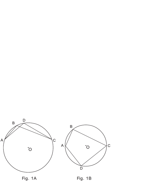
Figure 3.1: This figure shows the example for the case when crossed quadrangle(Fig.1A) has larger circumradius than that of convex quadrangle(Fig.1B) with same sides.

Consider a crossed-quadrangle $ABCD$ with sides $AB=a,BC=b,CD=c,DA=d$ that has circumcircle. It is easy to find the length of the interval $AC$

$$AC^{2}=\frac{(ac-bd)(bc-ad)}{ab-cd}.$$ (3.36)

This relation is true unless triangles $ABC$ and $ADC$ have the same height and as a consequence equal areas. Note that $S_{\times}$ is not an area of the crossed-quadrangle. It is the difference between the areas of the noted triangles.

Using Eq.(3.36), one can derive exactly Eq.(3.35) for the circumradius of the crossed-quadrangle.

Eq.(3.34) is meaningful if vectors ${\bm{u}}$ and ${\bm{v}}$ are unit and have nonzero components along the axis $y$.

3.3.3 Largest Coefficient

In this subsection we consider the last case described by Eq.(3.17). Entanglement eigenvalue takes maximal value if all terms in r.h.s. of Eq.(3.3) are positive. Then equations (3.17) and (3.10) together impose

$${\bm{u}}={\rm Sign}(r_{1}){\bm{k}},\quad{\bm{v}}={\rm Sign}(r_{2}){\bm{k}},\quad r_{1}r_{2}r_{3}<0,$$ (3.37)

where Sign(x) gives -1, 0 or 1 depending on whether x is negative, zero, or positive. Substituting these values into Eq.(3.3), we obtain

$$\Lambda_{\max}^{2}=\frac{1}{4}\left(1+|r_{1}|+|r_{2}|+|r_{3}|\right).$$ (3.38)

Owing to inequality, $r_{1}r_{2}r_{3}<0$, above expression always gives a square of the largest coefficient $l$

$$l=\max(a,b,c,d)$$ (3.39)

in Eq.(3.8). Indeed, let us consider the case $r_{1}>0,r_{2}>0,r_{3}<0$. From inequalities $r_{1}>0,r_{2}>0$ it follows that $c^{2}>d^{2}+|a^{2}-b^{2}|$ and therefore $c^{2}>d^{2}$. Note, $c^{2}>d^{2}$ is necessary but not sufficient condition. Now if $d>b$, then $r_{1}>0$ yields $c>a$ and if $d<b$, then $r_{3}<0$ yields $c>a$. Thus inequality $c>a$ is true in all cases. Similarly $c>b$ and $c$ is the largest coefficient. On the other hand $\Lambda_{\max}^{2}=c^{2}$ and Eq.(3.38) really gives the largest coefficient in this case.

Similarly, cases $r_{1}>0,r_{2}<0,r_{3}>0$ and $r_{1}<0,r_{2}>0,r_{3}>0$ yield $\Lambda_{\max}^{2}=b^{2}$ and $\Lambda_{\max}^{2}=a^{2}$, respectively. And again entanglement eigenvalue takes the value of the largest coefficient.

The last possibility $r_{1}<0,r_{2}<0,r_{3}<0$ can be analyzed using analogous speculations. One obtains $\Lambda_{\max}^{2}=d^{2}$ and $d$ is the largest coefficient.

Combining all cases mentioned earlier, we rewrite Eq.(3.38) as follows

$$\Lambda_{\max}^{2}=l^{2}.$$ (3.40)

This expression is valid if both vectors ${\bm{u}}$ and ${\bm{v}}$ are collinear with the axes $z$.

We have derived three expressions for (3.24),(3.34) and (3.40) for entanglement eigenvalue. They are valid when vectors ${\bm{u}}$ and ${\bm{v}}$ lie in $xz$ plane, lie in $yz$ plane and are collinear with axis $z$, respectively. The following section goes on to specify these domains by parameters $a,b,c,d$.

3.4 Applicable Domains

Mainly, two points are being analyzed. First, we probe into the meaningful geometrical interpretations of quantities $R_{q}$ and $R_{\times}$. Second, we separate validity domains of equations (3.24),(3.34) and (3.40). It is mentioned earlier that algebraic methods for solving the inequalities of degree six are ineffective. Hence, we use geometric tools that are elegant and concise in this case.

We consider four parameters $a,b,c,d$ as free parameters as the normalization condition is irrelevant here. Indeed, one can use the state $|\psi\rangle/\sqrt{a^{2}+b^{2}+c^{2}+d^{2}}$ where all parameters are free. If one repeats the same steps, the only difference is that the entanglement eigenvalue $\Lambda_{\max}^{2}$ is replaced by $\Lambda_{\max}^{2}/(a^{2}+b^{2}+c^{2}+d^{2})$. In other words, normalization condition re-scales the quadrangle, convex or crossed, so that the circumradius always lies in the required region. Consequently, in constructing quadrangles we can neglect the normalization condition and consider four free parameters $a,b,c,d$.

3.4.1 Existence of circumcircle.

It is known that four sides $a,b,c,d$ of the convex quadrangle must obey the inequality $p-l>0$. Any set of such parameters forms a cyclic quadrilateral. Note that the quadrangle is not unique as the sides can be arranged in different orders. But all these quadrangles have the same circumcircle and the circumradius is unique.

The sides of a crossed-quadrangle must obey the same condition. Indeed, from Fig.1A it follows that $BC-AB<AC<AD+DC$ and $DC-AD<AC<AB+BC$. Therefore $AB+AD+DC>BC$ and $AB+BC+AD>DC$. The sides $BC$ and $DC$ are two largest sides and consequently $p-l>0$. However, the existence of the circumcircle requires an additional condition and it is explained here. The relation $r_{3}=2\mu\cos ABC$ forces $4\mu^{2}\geq r_{3}^{2}$ and, therefore

$$S_{\times}^{2}\geq 0.$$ (3.41)

Thus the denominator in Eq.(3.35) must be positive. On the other hand the inequality $AC^{2}\geq 0$ forces a positive numerator of the same fraction

$$(ac-bd)(bc-ad)(ab-cd)\geq 0.$$ (3.42)

These two inequalities impose conditions on parameters $a,b,c,d$. For the future considerations, we need to write explicitly the condition imposed by inequality (3.42). The numerator is a symmetric function on parameters $a,b,c,d$ and it suffices to analyze only the case $a\geq b\geq c\geq d$. Obviously $(ac-bd)\geq 0,\,(ab-cd)\geq 0$ and it remains the constraint $bc\geq ad$. The last inequality states that the product of the largest and smallest coefficients must not exceed the product of remaining coefficients. Denote by $s$ the smallest coefficient

$$s=\min(a,b,c,d).$$ (3.43)

We can summarize all cases as follows

$$l^{2}s^{2}\leq abcd.$$ (3.44)

This is necessary but not sufficient condition for the existence of $R_{\times}$. The next condition $S_{\times}^{2}>0$ we do not analyze because the first condition (3.44) suffices to separate the validity domains.

3.4.2 Separation of validity domains.

In this section we define applicable domains of expressions (3.24),(3.34) and (3.40) step by step.

Circumradius of convex quadrangle.

First we separate the validity domains between the convex quadrangle and the largest coefficient. In a highly entangled region, where the center of circumcircle lies inside the quadrangle, the circumradius is greater than any of sides and yield a correct answer. This situation is changed when the center lies on the largest side of the quadrangle and both equations (3.24) and (3.40) give equal answers. Suppose that the side $a$ is the largest one and the center lies on the side $a$. A little geometrical speculation yields

$$a^{2}=b^{2}+c^{2}+d^{2}+2\frac{bcd}{a}.$$ (3.45)

From this equation we deduce that if $a^{2}$ is smaller than r.h.s., i.e.

$$a^{2}\leq b^{2}+c^{2}+d^{2}+2\frac{bcd}{a},$$ (3.46)

then the circumradius-formula is valid. If $a^{2}$ is greater than r.h.s in Eq.(3.45), then the largest coefficient formula is valid. The inequality (3.46) also guarantees the existence of the cyclic quadrilateral. Indeed, using the inequality

$$bc+cd+bd\geq 3\frac{bcd}{a},$$ (3.47)

one derives

$$(b+c+d)^{2}\geq b^{2}+c^{2}+d^{2}+\frac{6bcd}{a}\geq a^{2}.$$ (3.48)

Above inequality ensures the existence of a convex quadrangle with the given sides.

To get a confidence, we can solve equation $u_{k}=\pm 1$ using the relation (3.45). However, it is more transparent to factorize it as following:

$$(4\omega^{2}-r_{3}^{2})(1+u_{k}) = \frac{2ad}{bc+ad}\left(b^{2}+c^{2}+d^{2}+\frac{2bcd}{a}-a^{2}\right)$$ (3.49a)

$$\times \left(a^{2}+b^{2}+c^{2}+\frac{2abc}{d}-d^{2}\right)$$

$$(4\omega^{2}-r_{3}^{2})(1-u_{k}) = \frac{2bc}{bc+ad}\left(a^{2}+c^{2}+d^{2}+\frac{2acd}{b}-b^{2}\right)$$ (3.49b)

$$\times \left(a^{2}+b^{2}+d^{2}+\frac{2abd}{c}-c^{2}\right).$$

Similarly, we have

$$(4\omega^{2}-r_{3}^{2})(1+v_{k}) = \frac{2bd}{ac+bd}\left(a^{2}+c^{2}+d^{2}+\frac{2acd}{b}-b^{2}\right)$$ (3.50a)

$$\times \left(a^{2}+b^{2}+c^{2}+\frac{2abc}{d}-d^{2}\right)$$

$$(4\omega^{2}-r_{3}^{2})(1-v_{k}) = \frac{2ac}{ac+bd}\left(b^{2}+c^{2}+d^{2}+\frac{2bcd}{a}-a^{2}\right)$$ (3.50b)

$$\times \left(a^{2}+b^{2}+d^{2}+\frac{2abd}{c}-c^{2}\right).$$

Thus, the circumradius of the convex quadrangle gives a correct answer if all brackets in the above equations are positive. In general, Eq.(3.24) is valid if

$$l^{2}\leq\frac{1}{2}+\frac{abcd}{l^{2}}.$$ (3.51)

When one of parameters vanishes, i.e. $abcd=0$, inequality (3.51) coincides with the corresponding condition in Ref.[38].

Circumradius of crossed quadrangle.

Next we separate the validity domains between the convex and the crossed quadrangles. If $S_{\times}^{2}<0$, then crossed one has no circumcircle and the only choice is the circumradius of the convex quadrangle. If $S_{\times}^{2}>0$, then we use the equality

$$4R^{2}_{q}-4R^{2}_{\times}=\frac{r}{2}\frac{abcd}{S^{2}_{q}S^{2}_{\times}}$$ (3.52)

where $r=r_{1}r_{2}r_{3}$. It shows that $r>0$ yields $R_{q}>R_{\times}$ and vice-versa. Entanglement eigenvalue always takes the maximal value. Therefore, $\Lambda_{\max}^{2}=4R_{q}^{2}$ if $r>0$ and $\Lambda_{\max}^{2}=4R_{\times}^{2}$ if $r<0$. Thus $r=0$ is the separating surface and it is necessary to analyze the condition $r<0$.

Suppose $a\geq b\geq c\geq d$. Then $r_{2}$ and $r_{3}$ are positive. Therefore $r$ is negative if and only if $r_{1}$ is negative, which implies

$$a^{2}+d^{2}>b^{2}+c^{2}.$$ (3.53)

Now suppose $a\geq d\geq b\geq c$. Then $r_{1}$ is negative and $r_{3}$ is positive. Therefore $r_{2}$ must be positive, which implies

$$a^{2}+c^{2}>b^{2}+d^{2}.$$ (3.54)

It is easy to see that in both cases left hand sides contain the largest and smallest coefficients. This result can be generalized as follows: $r\leq 0$ if and only if

$$l^{2}\geq\frac{1}{2}-s^{2}.$$ (3.55)

It remains to separate the validity domains between the crossed-quadrangle and the largest coefficient. We can use three equivalent ways to make this separation:

1)to use the geometric picture and to see when $4R_{\times}^{2}$ and $l^{2}$ coincide,

2)directly factorize equation $u_{k}=\pm 1$,

3)change the sign of the parameter $d$.

All of these give the same result stating that Eq.(3.34) is valid if

$$l^{2}\leq\frac{1}{2}-\frac{abcd}{l^{2}}.$$ (3.56)

Inequalities (3.55) and (3.56) together yield

$$l^{2}s^{2}\geq abcd.$$ (3.57)

This inequality is contradicted by (3.44) unless $l^{2}s^{2}=abcd$. Special cases like $l^{2}s^{2}=abcd$ are considered in the next section. Now we would like to comment the fact that crossed quadrangle survives only in exceptional cases. Actually crossed case can be obtained from the convex cases by changing the sign of any parameter. It crucially depends on signs of parameters or, in general, on phases of parameters. On the other hand all phases in Eq.(3.8) can be eliminated by LU-transformations. For example, the phase of $d$ can be eliminated by redefinition of the phase of the state function $|\psi\rangle$ and the phases of remaining parameters can be absorbed in the definitions of basis vectors $|1\rangle$ of the qubits A, B and C. Owing to this entanglement eigenvalue being LU invariant quantity does not depend on phases. However, crossed case is relevant if one considers states given by Generalized Schmidt Decomposition(GSD) [48]. In this case phases can not be gauged away and crossed case has its own range of definition. This range has shrunk to the separating surface $r=0$ in our case.

Now we are ready to present a distinct separation of the validity domains:

$$\Lambda_{\max}^{2}=\begin{cases}\enskip 4R_{q}^{2},&{\rm if}\quad l^{2}\leq 1/2+abcd/l^{2}\cr\enskip l^{2}&{\rm if}\quad l^{2}\geq 1/2+abcd/l^{2}\end{cases}$$ (3.58)

As an illustration we present the plot of $d$-dependence of $\Lambda_{\max}^{2}$ in Fig.2 when $a=b=c$.

Figure 3.2: Plot of $d$-dependence of $\Lambda_{max}^{2}$ when $a=b=c$. When $d\to 1$, $\Lambda_{\max}^{2}$ goes to $1$ as expected. When $d=0$, $\Lambda_{\max}^{2}$ becomes $4/9$, which coincides with the result of Ref.[26]. When $r=0$ which implies $a=d=1/2$, $\Lambda_{\max}^{2}$ becomes $1/2$ (it is shown as dotted line). When $d=2a$, which implies $d=\sqrt{4/7}$, $\Lambda_{\max}^{2}$ goes to $4/7$, which is one of shared states (it is also shown as another dotted line).

We have distinguished three types of quantum states depending on which expression takes entanglement eigenvalue. Also there are states that lie on surfaces separating different applicable domains. They are shared by two types of quantum states and may have interesting features. We will call those shared states. Such shared states are considered in the next section.

3.5 Shared States.

Consider quantum states for which both convex and crossed quadrangles yield the same entanglement eigenvalue. Eq.(3.36) is not applicable and we rewrite equations (3.27) and (3.35) as follows

$$4R_{q}^{2}=\frac{1}{2}\left(1-\frac{r}{16S^{2}_{q}}\right),\quad 4R_{\times}^{2}=\frac{1}{2}\left(1-\frac{r}{16S^{2}_{\times}}\right).$$ (3.59)

These equations show that if the state lies on the separating surface $r=0$, then entanglement eigenvalue is a constant

$$\Lambda_{\max}^{2}=\frac{1}{2}$$ (3.60)

and does not depend on the state parameters. This fact has a simple interpretation. Consider the case $r_{1}=0$. Then $b^{2}+c^{2}=a^{2}+d^{2}=1/2$ and the quadrangle consists of two right triangles. These two triangles have a common hypotenuse and legs $b,c$ and $a,d$, respectively, regardless of the triangles being in the same semicircle or in opposite semicircles. In both cases they yield same circumradius. Decisive factor is that the center of the circumcircle lies on the diagonal. Thus the perimeter and diagonals of the quadrangle divide ranges of definition of the convex quadrangle. When the center of circumcircle passes the perimeter, entanglement eigenvalue changes-over from convex circumradius to the largest coefficient. And if the center lies on the diagonal, convex and crossed circumradiuses become equal.

We would like to bring plausible arguments that this picture is incomplete and there is a region that has been shrunk to the point. Consider three-qubit state given by GSD

$$|\psi\rangle=a|100\rangle+b|010\rangle+b|001\rangle+d|111\rangle+e|000\rangle.$$ (3.61)

One of parameters must have non-vanishing phase[48] and we can treat this phase as an angle. Then, we have five sides and an angle. This set defines a sexangle that has circumcircle. One can guess that in a highly entangled region entanglement eigenvalue is the circumradius of the sexangle. However, there is a crucial difference. Any convex sexangle contains a star type area and the sides of this area are the diagonals of the sexangle. The perimeter of the star separates the convex and the crossed cases. Unfortunately, we can not see this picture in our case because the diagonals of a quadrangle confine a single point. It is left for future to calculate the entanglement eigenvalues for arbitrary three qubit states and justify this general picture.

Shared states given by $r=0$ acquire new properties. They can be used for perfect teleportation and superdense coding [38, 63]. This statement is not proven clearly, but also no exceptions are known.

Now consider a case where the largest coefficient and circumradius of the convex quadrangle coincide with each other. The separating surface is given by

$$l^{2}=\frac{1}{2}+\frac{abcd}{l^{2}}.$$ (3.62)

Entanglement eigenvalue ranges within the narrow interval

$$\frac{1}{2}\leq\Lambda_{\max}^{2}\leq\frac{4}{7}.$$ (3.63)

It separates slightly and highly entangled states. When one of coefficients is large enough and satisfies the relation $l^{2}>1/2+abcd/l^{2}$, entanglement eigenvalue takes a larger coefficient. And the expression (3.8) for the state function effectively takes the place of Schmidt decomposition. In highly entangled region no similar picture exists and all coefficients participate in equal parts and yield the circumradius. Thus, shared states given by Eq.(3.62) separate slightly entangled states from highly entangled ones, and can be ascribed to both types.

What is the meaning of these states? Shared states given by $r=0$ acquire new and important features. One can expect that shared states dividing highly and slightly entangled states also must acquire some new features. However, these features are yet to be discovered.

3.6 Conclusions

We have considered four-parametric families of three qubit states and derived explicit expressions for entanglement eigenvalue. The final expressions have their own geometrical interpretation. The result in this paper with the results of Ref.[38] show that the geometric measure has two visiting cards: the circumradius and the largest coefficient. The geometric interpretation may enable us to predict the answer for the states given by GSD. If the center of circumcircle lies in star type area confined by diagonals of the sexangle, then entanglement eigenvalue is the circumradius of the crossed sexangle(s). If the center lies in the remaining part of sexangle, the entanglement eigenvalue is the circumradius of the convex sexangle. And when the center passes the perimeter, then entanglement eigenvalue is the largest coefficient. Although we cannot justify our prediction due to lack of computational technique, this picture surely enables us to take a step toward a deeper understanding of the entanglement measure.

Shared states given by $r=0$ play an important role in quantum information theory. The application of shared states given by Eq.(3.62) is somewhat questionable, and should be analyzed further. It should be pointed out that one has to understand the properties of these states and find the possible applications. We would like to investigate this issue elsewhere.

Finally following our procedure, one can obtain the nearest product state of a given three-parametric W-type state. These two states will always be separated by a line of densities composed of the convex combination of W-type states and the nearest product states [70]. There is a separable density matrix $\varrho_{0}$ which splits the line into two parts as follows. One part consists of separable densities and another part consists of non-separable densities. It was shown in Ref.[70] that an operator $W=\varrho_{0}-\rho^{ABC}-\mathrm{tr}[\varrho_{0}(\varrho_{0}-\rho^{ABC})]I$ has the properties $\mathrm{tr}(W\rho^{ABC})<0$, and $\mathrm{tr}(W\varrho)\geq 0$ for the arbitrary separable state $\varrho$. The operator $W$ is clearly Hermitian and thus is an entanglement witness for the state. Thus our results allow oneself to construct the entanglement witnesses for W-type three qubit states. However, the explicit derivation of $\varrho_{0}$ seems to be highly non-trivial.

Chapter 4 Duality and the geometric measure of entanglement of general multiqubit W states

In this chapter we find the nearest product states and geometric measure of entanglement for arbitrary generalized W states of $n$ qubits [31, 76].

Quantifying entanglement of multipartite pure states presents a real challenge to physicists. Intensive studies are under way and different entanglement measures have been proposed over the years [23, 24, 77, 78, 79, 80, 81]. However, it is generally impossible to calculate their value because the definition of any multipartite entanglement measure usually includes a massive optimization over certain quantum protocols or states [21, 38, 82].

Inextricable difficulties of the optimization are rooted in a tangle of different obstacles. First, the number of entanglement parameters grows exponentially with the number of particles involved [83]. Second, in the multipartite setting several inequivalent classes of entanglement exist [50, 84]. Third, the geometry of entangled regions of robust states is complicated [43]. All of these make the usual optimization methods ineffective [30, 43, 45]. Concise and elegant tools are required to overcome this problem.

A widely used measure for multipartite systems is the maximal product overlap $\Lambda_{max}$. In what follows states with $\Lambda_{\max}^{2}>1/2$ are referred to as slightly entangled, states with $\Lambda_{\max}^{2}<1/2$ are referred to as highly entangled and states with $\Lambda_{\max}^{2}=1/2$ are referred to as shared quantum states. In this chapter we show how to calculate the maximal product overlap of an arbitrary W state [50]. The method is to establish a one-to-one correspondence between highly entangled W states and their nearest product states.

Consider first generalized Greenberger-Horne-Zeilinger states [49], i.e. states that can be written $|\mathrm{GHZ}\rangle=a|0\ldots 0\rangle+b|1\ldots 1\rangle$ in some product basis. Such states are fragile under local decoherence, i.e. they become disentangled by the loss of any one party, and they are not highly entangled in the sense defined above. The geometric measure of these states is computed easily since the maximal overlap simply takes the value of the modulus of the larger coefficient, $|a|$ or $|b|$ [61]. Accordingly, the nearest separable state is the product state with the larger coefficient. Thus many generalized GHZ states with different maximal overlaps can have the same nearest product state.

Consider now generalized W-states [85], which can be written

$$|\mathrm{W}_{n}\rangle=c_{1}|100...0\rangle+c_{2}|010...0\rangle+\cdots+c_{n}|00...01\rangle.$$ (4.1)

Without loss of generality we consider only the case of positive parameters $c_{k}$ since the phases of the coefficients $c_{k}$ can be eliminated by redefinitions of local states $|1_{k}\rangle,\,k=1,2,...,n$. The states (4.1) are robust against decoherence [86], i.e. loss of any $n-2$ parties still leaves them in a bipartite entangled state. Surprisingly, if the state is slightly entangled, then we have the same situation as for generalized GHZ states: the maximal overlap is the largest coefficient and, as before, many states can have the same nearest product state [76]. However, the situation is changed drastically when the state is highly entangled. The calculation of the maximal overlap in this case is a very difficult problem and the maximization has been performed only for relatively simple systems [26, 30, 38, 61, 76, 87, 88, 89].

On the other hand, different highly entangled W-states have different nearest product states. This makes it possible to map the W-state to its nearest product state and quickly obtain its geometric measure of entanglement. More precisely, we construct two bijections. The first one creates a map between highly entangled $n$-qubit W states and $n$-dimensional unit vectors $\mathbf{x}$. The second one does the same between $n$-dimensional unit vectors and $n$-part product states. Thus we obtain a double map, or duality, as follows

$$|\mathrm{W}_{n}\rangle\;\leftrightarrow\;\mathbf{x}\;\leftrightarrow\;|u_{1}\rangle\otimes|u_{2}\rangle\otimes\cdots\otimes|u_{n}\rangle.$$ (4.2)

The main advantage of the map is that if one knows any of the three vectors, then one instantly finds the other two.

This chapter is organized as follows. In Section 4.1 we construct a classifying map. In Section 4.2 we consider highly entangled multi-qubit W states. In Section 4.3 we derive a closed-form expression for the maximal overlap of n-qubit W states. In Section 4.4 we summarize our results.

4.1 Classifying map.

Now we prove a theorem that provides a basis for the map.

Theorem 1.

Let $|\mathrm{W}_{n}\rangle$ be an arbitrary W state (4.1) with non-negative real coefficients $c_{i}$, and let $|u_{1}\rangle\otimes|u_{2}\rangle\otimes\cdots\otimes|u_{n}\rangle$ be its nearest product state. Then the phase of $|u_{k}\rangle$ can be chosen so that

$$|u_{k}\rangle=\sin\theta_{k}|0\rangle+\cos\theta_{k}|1\rangle,\,0\leq\theta_{k}\leq\frac{\pi}{2},\,k=1,2,...,n.$$

where

$$\cos^{2}\theta_{1}+\cos^{2}\theta_{2}+\cdots+\cos^{2}\theta_{n}=1.$$ (4.3)

Proof.

The nearest product state is a stationary point for the overlap with $|\mathrm{W}_{n}\rangle$, so the states $|u_{k}\rangle$ satisfy the nonlinear eigenvalue equations [26, 39, 38]

$$\langle u_{1}u_{2}\cdots\widehat{u_{k}}\cdots u_{n}|\mathrm{W}_{n}\rangle=\Lambda_{max}|u_{k}\rangle;\;k=1,2,\cdots,n$$ (4.4)

where the caret means exclusion. We can choose the phase of $|u_{k}\rangle$ so that $|u_{k}\rangle=\sin\theta_{k}|0\rangle+\mathrm{e}^{i\phi_{k}}\cos\theta_{k}|1\rangle,$ and then (4.4) gives the pair of equations

$$c_{k}\prod_{j\neq k}\sin\theta_{j}=\Lambda_{max}\mathrm{e}^{i\phi_{k}}\cos\theta_{k},$$ (4.5a)

$$\sum_{l\neq k}\mathrm{e}^{-i\phi_{l}}c_{l}\cos\theta_{l}\prod_{j\neq k,l}\sin\theta_{j}=\Lambda_{max}\sin\theta_{k}.$$ (4.5b)

Eq. (4.5a) shows that $\Lambda_{max}\mathrm{e}^{i\phi_{k}}$ is real, so $\phi_{k}=-\arg(\Lambda_{max})$ is independent of $k$. Then the modulus of the overlap $|\langle u_{1}\cdots u_{n}|\mathrm{W}_{n}\rangle|$ is independent of $\phi$, so we can assume that $\phi=0$. Now multiplying eq.(4.5b) by $\sin\theta_{k}$ and using eq.(4.5a) gives Eq.(4.3). ∎

Thus the angles $\cos\theta_{k}$ define a unit $n$-dimensional Euclidean vector $\mathbf{x}$. We can also define a length $r$ as follows. From Eq.(4.5a) it follows that the ratio $\sin 2\theta_{k}/c_{k}$ does not depend on $k$. If this ratio is non-zero we can define

$$\frac{1}{r}\equiv\frac{\sin 2\theta_{1}}{c_{1}}=\frac{\sin 2\theta_{2}}{c_{2}}=\cdots=\frac{\sin 2\theta_{n}}{c_{n}}.$$ (4.6)

4.2 Highly entangled W states.

Equations (5) admit a trivial solution $\sin 2\theta_{k}=0,\,k=1,2,\cdots,n$ and a special solution with nonzero values of all sines. The trivial solution gives the largest coefficient of $|\mathrm{W}_{n}\rangle$ for the maximal overlap and is valid for slightly entangled states. We consider them later and now focus on the special solutions. From Eq.(4.6) it follows that

$$\cos^{2}\theta_{k}=\frac{1}{2}\left(1\pm\sqrt{1-\frac{c_{k}^{2}}{r^{2}}}\right),\;k=1,2,\cdots,n.$$ (4.7)

The plus sign means that $\cos 2\theta_{k}>0$. Then from Eq.(4.3) it follows that this is possible for at most one angle; specifically, we prove that if $\cos 2\theta_{k}>0$ for some $k$, then $c_{k}$ is the largest coefficient in Eq.(4.1). Suppose $\cos 2\theta_{k}>0$ but $c_{k}$ is not the largest coefficient and there exists a greater coefficient, say $c_{l}$. Then from Eq.(4.6) it follows that $\sin 2\theta_{l}>\sin 2\theta_{k}>0$ and consequently $|\cos 2\theta_{l}|<|\cos 2\theta_{k}|$. Now we rewrite Eq.(4.3) as follows:

$$-\cos 2\theta_{1}-\cos 2\theta_{2}-\cdots-\cos 2\theta_{n}=n-2.$$ (4.8)

From $|\cos 2\theta_{l}|<|\cos 2\theta_{k}|$ and $\cos 2\theta_{k}>0$ it follows that $-\cos 2\theta_{k}-\cos 2\theta_{l}<0$ which is in contradiction with Eq.(4.8). Thus $c_{k}$ must be the largest coefficient.

Without loss of generality we assume that $0\leq c_{1}\leq\cdots\leq c_{n}$. Then in (4.7) we must take the $-$ sign for $k=1,\ldots,n-1$ and (4.3) becomes

$$\sqrt{1-\frac{c_{1}^{2}}{r^{2}}}+\cdots+\sqrt{1-\frac{c_{n-1}^{2}}{r^{2}}}\pm\sqrt{1-\frac{c_{n}^{2}}{r^{2}}}=n-2$$ (4.9)

We will denote the left-hand sides of these equations as $f_{\pm}(r)$. We also use $f_{0}(r)$ to denote this expression without the last term. The function $r(c_{1},c_{2},...,c_{n})$ defined by $f_{+}(r)=n-2$ is a completely symmetric function of the state parameters $c_{k}$. In contrast, the function defined by $f_{-}(r)=n-2$ is an asymmetric function since its dependence on the maximal coefficient $c_{n}$ is different. Thus in equation (4.9) the upper and lower signs describe symmetric and asymmetric entangled regions of highly entangled states, respectively.

For highly entangled states, eqs. (4.9)_± uniquely define $r$ as a function of the state parameters $c_{k}$. More precisely,

Theorem 2.

There are two critical values $r_{1}$ and $r_{2}$ of the largest coefficient $c_{n}$, i.e. functions of $c_{1},\ldots,c_{n-1}$ such that

1. If $c_{n}\leq r_{1}$, there is a unique solution of (4.9₊) and no solution of (4.9_-);

2. If $c_{n}=r_{1}$, both (4.9₊) and (4.9_-) have a unique solution, the same for both;

3. If $r_{1}<c_{n}\leq r_{2}$, there is no solution of (4.9)₊ and a unique solution of (4.9_-);

4. If $c_{n}>r_{2}$, neither (4.9₊) nor (4.9_-) has a solution. In this case the state $|\mathrm{W}_{n}\rangle$ is slightly entangled.

The value $r_{1}$ is the solution of $f_{0}(r_{1})=n-2$, which exists and is unique since $f_{0}(c_{n-1})<n-2$ and $f_{0}(r)\rightarrow n-1$ monotonically as $r\rightarrow\infty$; and $r_{2}$ is defined by

$$r_{2}^{2}=c_{1}^{2}+\cdots+c_{n-1}^{2}.$$ (4.10)

Then $r_{2}\geq r_{1}$, for $f_{0}(r_{2})\geq n-2=f_{0}(r_{1})$ using $\sqrt{x}\geq x$ for $0\leq x\leq 1$. Since $f_{0}$ is an increasing function of $r,$ it follows that $r_{2}\geq r_{1}$. Now the theorem follows from the following properties of the functions $f_{\pm}(r)$($f^{\prime}_{-}$ is the derivative of $f_{-}$):

1. $f_{0}$ and $f_{+}$ are monotonically increasing functions of $r$.

2. $f_{+}(r)\rightarrow n$ as $r\rightarrow\infty$.

3. If $c_{n}\leq r_{1}$, $f_{+}(c_{n})=f_{0}(c_{n})\leq f_{0}(r_{1})=n-2$.

4. If $c_{n}\geq r_{1}$, then $f_{+}(r)\geq n-2$ for all $r>r_{1}$.

5. If $c_{n}<r_{1}$, then $f_{-}(c_{n})<n-2$.

6. If $c_{n}>r_{1}$, then $f_{-}(c_{n})>n-2$.

7. If $c_{n}<r_{2}$, then $f_{-}(r)<n-2$ for large $r$.

8. If $c_{n}>r_{2}$ then $f_{-}(r)>n-2$ for large $r$.

9. $f^{\prime}_{-}(c_{n}+\epsilon)<0$ for small $\epsilon$.

​​​10. If $c_{n}>r_{2}$, then $f^{\prime}_{-}(r)<0$ for all $r\geq c_{n}$.

These properties are illustrated in Figure 4.1.

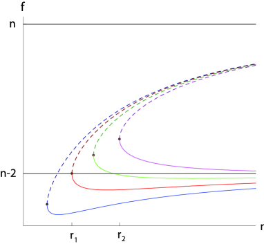
Figure 4.1: (Color online) The behaviour of the functions $f_{\pm}$ for five-qubit W states. The function $f_{+}(r)$ (dotted line) and $f_{-}(r)$ (solid line) are plotted against $r$ in the four cases $c_{n}<r_{1}$, $c_{n}=r_{1}$, $r_{1}<c_{n}<r_{2}$ and $c_{n}=r_{2}$.

4.3 Geometric measure.

We can now identify the nearest product state, and the largest product state overlap $\Lambda_{max}(|\mathrm{W}_{n}\rangle)$, for any W-state $|\mathrm{W}_{n}\rangle$, as follows.

Theorem 3.

If $c_{n}\geq 1/2$, the state $|\mathrm{W}_{n}\rangle$ defined by (4.1) is slightly entangled. Its nearest product state is $|0\ldots 01\rangle$, with overlap $\Lambda_{max}(|\mathrm{W}_{n}\rangle)=c_{n}$.

If $c_{n}\leq 1/2$, the state $|\mathrm{W}_{n}\rangle$ is highly entangled and has nearest product state

$$|u_{1}\rangle\ldots|u_{n}\rangle\;\;\text{ where }\;\;|u_{k}\rangle=\sin\theta_{k}|0\rangle+|\mathrm{e}^{i\phi}\cos\theta_{k}|1\rangle,$$ (4.11)

with which its overlap is

$$\Lambda_{max}=2r\sin\theta_{1}\sin\theta_{2}\ldots\sin\theta_{n}.$$ (4.12)

Here $r$ is the solution of (4.9)_±, whose existence and uniqueness are guaranteed by Theorem 2; the phase $\phi$ is arbitrary; and $\theta_{k}$ is given by (4.7) with the $-$ sign for $k=1,\ldots,n-1$, the $-$ sign for $k=n$ if $r$ satisfies (4.9₊), the $+$ sign if $r$ satisfies (4.9_-).

Proof.

The nonlinear eigenvalue equations (4.4) always have $n$ solutions

$$\Lambda_{max}=c_{k},\qquad|u_{i}\rangle=\begin{cases}|0\rangle\text{ if }i\neq k,\\ |1\rangle\text{ if }i=k\end{cases},\quad k=1\ldots n$$

If $c_{n}\geq\/2$, i.e. in case (4) of Theorem 2, there are no other stationary values, so the largest overlap $\Lambda_{max}(|\mathrm{W}_{n}\rangle)$ equals the largest coefficient $c_{n}$, the corresponding product state being $|0\ldots 01\rangle$.

If $c_{n}<1/2$ there is another stationary value given by (4.12). We will now show that this is larger than any of the trivial stationary values $c_{k}$. We use the following inequality: If $y_{1},\ldots,y_{n}$ are real numbers lying between 0 and 1, and satisfying $y_{1}+\cdots+y_{n}\leq 1$, then

$$(1-y_{1})(1-y_{2})\cdots(1-y_{n})\geq 1-y_{1}-y_{2}-\ldots-y_{n}.$$ (4.13)

This is readily proved by induction. We can apply (4.13) to $n-1$ terms of Eq.(4.3) to get

$$(1-\cos^{2}\theta_{1})\cdots(1-\cos^{2}\theta_{n-1})\geq 1-\cos^{2}\theta_{1}-\cdots-\cos^{2}\theta_{n-1}$$

or

$$\sin^{2}\theta_{1}\sin^{2}\theta_{2}\sin^{2}\theta_{n-1}\geq\cos^{2}\theta_{n}.$$ (4.14)

Now from Eq.(4.5a) it follows that $\Lambda_{\max}^{2}\geq c_{n}^{2}$. Thus $\Lambda_{max}$ is the maximal product overlap, and the nearest product state is $|u_{1}\rangle\ldots u_{n}\rangle$.

Next we prove that if $|\mathrm{W}_{n}\rangle$ is normalised, then $\Lambda_{\max}^{2}<1/2$. For this we need another inequality: If $y_{1},\ldots,y_{n}$ are real numbers lying between 0 and 1, and satisfying $y_{1}+\cdots+y_{n}=n-1$, then

$$y_{1}+\cdots+y_{n}\geq y_{1}^{2}+\cdots+y_{n}^{2}+2y_{1}y_{2}\ldots y_{n}.$$ (4.15)

This can also be proved by induction.

From (4.6), and using $c_{1}^{2}+\cdots+c_{n}^{2}=1$, we find

$$r^{2}=\frac{1}{\sin^{2}2\theta_{1}+\cdots+\sin^{2}2\theta_{n}}.$$ (4.16)

Hence (4.12) gives

$$\Lambda_{\max}^{2}=\frac{y_{1}y_{2}\ldots y_{n}}{y_{1}(1-y_{1})+\cdots y_{n}(1-y_{n})}$$ (4.17)

where $y_{k}=\sin^{2}\theta_{k}$. But $y_{1}+\cdots+y_{n}=n-1$, so the inequality (4.15) applies, and gives $\Lambda_{\max}^{2}\leq 1/2$. ∎

Finally, we summarise the correspondence between highly entangled W-states, their nearest product states, and unit vectors in $\mathbb{R}^{n}$.

Theorem 4.

There is a 1:1 correspondence between highly entangled states $|\mathrm{W}_{n}\rangle$ defined by (4.1), their nearest product states with real non-negative coefficients, and unit vectors $\mathbf{x}\in\mathbb{R}^{n}$ with $0<x_{k}<1/\sqrt{2}$ ($k=1,\ldots,n-1$), $0<x_{n}<1$.

Proof.

By Theorem 3, $|\mathrm{W}_{n}\rangle$ is highly entangled if and only if $c_{n}<1/2$. If this is the case, Theorem 1 and (4.7) show that its nearest product state is of the form (4.11) where $\mathbf{x}=(\cos\theta_{1},\ldots,\cos\theta_{n})$ is a unit vector in $\mathbb{R}^{n}$ in the region stated. The angles $\theta_{k}$ are given in terms of the coefficients $c_{k}$ by (4.6), in which $r$ is a function of the coefficients which, by Theorem 2, is uniquely defined. The nearest product states $|u_{1}\rangle|u_{2}\rangle\ldots|u_{n}\rangle$ are determined by these angles, up to a phase $\phi$, by $|u_{k}\rangle=\sin\theta_{k}|0\rangle+\mathrm{e}^{i\phi}\cos\theta_{k}|1\rangle$, so there is only one nearest product state with real non-negative coefficients, and only one unit vector $\mathbf{x}$, for each highly entangled state $|\mathrm{W}_{n}\rangle$. Conversely, given a unit vector $\mathbf{x}=(\cos\theta_{1},\ldots,\cos\theta_{n})$, the quantity $r$ is determined by (4.16), and then the coefficients $c_{1},\ldots,c_{n}$ are determined by (4.6). Thus the correspondences (4.2) are bijections. ∎

The equations (4.9_±) cannot always be explicitly solved to give analytic expressions for $r$ in terms of the coefficients $c_{k}$. However, in some cases, including all states for $n=3$, explicit solutions can be obtained. Then the angles $\theta_{k}$ can be calculated from (4.6) and eq.(4.12) gives a formula for the maximal product overlap $\Lambda_{max}(|\mathrm{W}_{n}\rangle)$. This formula is valid unless any of the angles $\theta_{k}$ vanishes, and restores all known results for the maximal overlap of highly entangled W states. When $n=3$ it coincides with the formula (31) in Ref.[38]. When $c_{1}=c_{2}=\cdots=c_{n}$ it coincides with the formula (52) in Ref.[62]. And when $n=4$ and $c_{3}=c_{4}$ it coincides with the formula (37) derived in Ref.[76].

When $\max(c_{1}^{2},c_{2}^{2},\cdots c_{n}^{2})=r_{2}^{2}=1/2$ the two expressions for $\Lambda_{max}(|\mathrm{W}_{n}\rangle)$ given in Theorem 3 coincide; these states are shared quantum states. The nearest product states and maximal overlaps of shared states are given by the first case of Theorem 3, but also they appear as asymptotic limits of the second case. Indeed, at the limit $\theta_{n}\to 0$ we have

$$\lim_{\theta_{n}\to 0}2r\sin\theta_{n}\to c_{n},\;\lim_{\theta_{n}\to 0}2r\cos\theta_{k}\to c_{k},\,k\neq n.$$ (4.18)

Thus the angle $\theta_{n}$ vanishes and the length of the vector ${\bm{r}}$ goes to infinity, but their product has a finite limit. Substituting these limits into Eq.(4.3) one obtains $c_{n}^{2}\to r_{2}^{2}$. Therefore entangled regions of highly and slightly entangled states are separated by the surface $c_{n}^{2}=1/2$; for states on the surface, $r\to\infty$. All of these states can be used as a quantum channel for the perfect teleportation and superdense coding [43].

4.4 Summary.

We have constructed correspondences between W states, $n$-dimensional unit vectors and separable pure states. The map reveals two critical values for quantum state parameters. The first critical value separates symmetric and asymmetric entangled regions of highly entangled states, whiles the second one separates highly and slightly entangled states. The method gives an explicit expressions for the geometric measure when the state allows analytical solutions, otherwise it expresses the entanglement as an implicit function of state parameters.

It should be noted that the bijection between W states and $n$-dimensional unit vectors is not related directly to the geometric measure of entanglement. Therefore it is possible to extend the method to other entanglement measures. To this end one creates an appropriate bijection between unit vectors and optimization points of an entanglement measure one wants to compute.

Chapter 5 Universal behavior of the geometric entanglement measure of many-qubit W states

In this chapter we analyze geometric entanglement measure of many-qubit W states and derive an interpolating formula [52].

The physics of many-particle systems differs fundamentally from the one of a few particles and gives rise to new interesting phenomena, such as phase transitions [36, 53] or quantum computing [4, 6, 10, 56]. Entanglement theory, in particular, appears to have a much more complex and richer structure in the N-partite case than it has in the bipartite setting. This is reflected by the fact that multipartite entanglement is a very active field of research that has led to important insights into our understanding of many-particle physics [24, 26, 39, 90, 91, 92, 93, 94]. In view of this, it seems worthy to investigate also the behavior of entanglement measures for large-scale systems. Despite the fact that the number of entanglement parameters scales exponentially in the number of particles [57], it is sometimes possible to capture the most relevant physical properties by describing these systems in terms of very few parameters.

Recently a duality between highly entangled W states and product states has been established [31]. The important class of W states [50] represents a particular interesting set of quantum states associated with high robustness against particle loss and nonlocal properties of genuine entangled multipartite states [85, 95, 96, 97]. And different experimentally accessible schemes to generate multipartite W states have been proposed and put into practice over the years [86, 98, 99, 100]

The duality specifies a single-valued function $r$ of entanglement parameters. We shall refer to $r$ as the entanglement diameter, as it will play a crucial role throughout this article. Another reason for the term entanglement diameter is that $r$ can be interpreted geometrically as a diameter of a circumscribing sphere. The geometrical interpretation and its illustration will be presented in the appendix and now we focus on the physical significance of $r$.

The entanglement diameter uniquely defines the maximal product overlap and nearest product state [23, 25, 26, 29] of a given highly entangled W state. It has two exceptional points in the parameter space of W states. At the second exceptional point the reduced density operator of a some qubit is a constant multiple of the unit operator and then the entanglement diameter becomes infinite. The maximal product overlap $\Lambda_{max}$ of these states is a constant regardless how many qubits are involved and what are the values of the remaining entanglement parameters. These states are known as shared quantum states and can be used as quantum channels for the perfect teleportation and dense coding. Thus the shared quantum states are uniquely defined as the states whose entanglement diameter is infinite.

Furthermore, highly entangled W states have two different entangled regions: the symmetric and asymmetric entangled regions. In the computational basis these regions can be defined as follows. If a W state is in the symmetric region, then the entanglement diameter is a fully symmetric function on the state parameters. Conversely, if a W state is in the asymmetric region, then there is a coefficient $c$ such that the $c$ dependence of the entanglement diameter differs dramatically from the dependencies of the remaining coefficients. Hence the point of intersection of the symmetric and asymmetric regions is the first exceptional point. It depends on state parameters and its role has not been revealed so far. One thing was clear that the first exceptional point does not play an important role for three- and four-qubit W states [38, 76].

In this chapter we show that the first exceptional point is important for large-scale W states. It approaches to a fixed point when number of qubits $N$ increases and becomes state-independent(up to $1/N$ corrections) when $N\gg 1$. As a consequence the entanglement diameter, as well as the maximal product overlap, becomes state-independent too and therefore many-qubit W states have two state-independent exceptional points. The underlying concept is that states whose entanglement parameters differ widely, may nevertheless have the same maximal product overlap and this phenomenon should occur at two fixed points. This is an analog of the universality of dynamical systems at critical points. It is an intriguing fact that systems with quite different microscopic parameters may behave equivalently at criticality. Fortunately, the renormalization group provides an explanation for the emergence of universality in critical systems [36, 37, 53].

The developed concept distinguishes three classes of W states. The first class consists of highly entangled W states which are below both exceptional points and then $r$ varies from $r_{\min}=1/2$ to $r_{0}\approx 1/\sqrt{3}+O(1/N)$. We will show that these states are in the symmetric region and their entanglement diameter is a slowly oscillating function on entanglement parameters. Accordingly, the maximal product overlap is an almost everywhere constant close to its greatest lower bound. Similar results have been obtained in Ref.[89], where it is shown that almost all multipartite pure states with sufficiently large number of parties are nearly maximally entangled with respect to the geometric measure [26] and relative entropy of entanglement [24]. We will not analyze rigorously these states since they are too entangled to be useful in quantum information theory [63].

The second and most interesting class consists of highly entangled W states which are between two exceptional points and then $r$ varies from $r_{0}$ to infinity. These states are in the asymmetric region and the behavior of the entanglement diameter is curious. We will show that $r$ is a one-variable function in this case and depends only on the Bloch vector ${\bm{b}}$ of a single qubit. As a consequence $\Lambda_{max}$ depends only on the same Bloch vector too and its behavior is universal. That is, regardless how many many qubits are involved and what are the remaining $N-1$ entanglement parameters the function $\Lambda_{max}({\bm{b}})$ is common. We will compute analytically $\Lambda_{max}({\bm{b}})$ and thereby find the Groverian and geometric entanglement measures [26, 29] for the large-scale W states even if neither the number of particles nor the most of state parameters are known.

The third class consists of slightly entangled W states which are above both exceptional points. In this case the maximal product overlap takes the value of the largest coefficient and these states do not posses an entanglement diameter. We will not analyze this trivial case, but will combine the functions $\Lambda_{max}({\bm{b}})$ for slightly entangled and highly entangled asymmetric W states and obtain an interpolating function $\Lambda_{max}({\bm{b}})$ valid for both cases. It is in a perfect agreement with numerical solutions and quantifies the many-qubit entanglement in high accuracy($\Delta\Lambda_{max}/\Lambda_{max}\sim 10^{-3}$ at $N\sim 10)$.

The importance of the interpolating formula in quantum information is threefold. First, it connects two quantities, namely the Bloch vector and maximal product overlap, that can be easily estimated in experiments [35, 102]. Second, it is an example of how do we compute entanglement of a quantum state with many unknowns. Third, if the Bloch vector varies within the allowable domain then maximal product overlap ranges from its lower to its upper bounds. Then one can prepare the W state with the given maximal product overlap, say ${\Lambda_{max}}_{0}$, bringing into the position the Bloch vector, say $\Lambda_{max}({\bm{b}_{0}})={\Lambda_{max}}_{0}$.

This chapter is organized as follows. In Section 5.1, we review the main results of Ref.[31]. In Section 6.2, we consider two- and three-parameter W states in the symmetric region and show that all of these states are almost maximally entangled. In Section 5.3, we consider three- and four-parameter W states in the asymmetric region and compute explicitly their maximal product overlap. In Section 5.4, we generalize the results of Sec.III and Sec.IV to arbitrary many-qubit W states. In Section 5.5, we discuss our results. In the Appendix C, we provide a geometrical interpretation for the entanglement diameter.

5.1 Maximal product overlap of W states

In the computational basis N-qubit W states can be written as

$$|\mathrm{W}_{n}\rangle=c_{1}|100...0\rangle+c_{2}|010...0\rangle+\cdots+c_{N}|00...01\rangle,$$ (5.1)

where the labels within kets refer to qubits 1,2,…,N in that order. The phases of the coefficients $c_{k}$ can be absorbed in the definitions of the local states $|1_{i}\rangle(i=1,2,...,N)$ and without loss of generality we consider only the case of positive parameters. For the simplicity we assume that $c_{N}$ is the maximal coefficient, that is, $c_{N}=\max(c_{1},c_{2},\cdots,c_{N})$.

The maximal product overlap $\Lambda_{max}(\psi)$ of a pure state $|\psi\rangle$ is given by

$$\Lambda_{max}(\psi)=\max_{u_{1},u_{2},...,u_{N}}|\left\langle\psi|u_{1}u_{2}...u_{N}\right\rangle|,$$ (5.2)

where the maximization runs over all product states. The larger $\Lambda_{max}$ is, the less entangled is $|\psi\rangle$. Hence for a quantum multipartite system the geometric entanglement measure $E_{\Lambda_{max}}$ is defined as

$$E_{\Lambda_{max}}=-\log\Lambda_{max}(\psi).$$

The maximal product overlap demarcates three different entangled regions in the parameter space of W states:

1. The symmetric region of highly entangled W states. Here $\Lambda_{max}(c_{1},c_{2},...,c_{N})$ is a symmetric function on all coefficients $c_{i}$.

2. The asymmetric region of highly entangled W states. Here the invariance of $\Lambda_{max}(c_{1},c_{2},...,c_{N})$ under the permutations of coefficients $c_{i}$ ceases to be true.

3. The region of slightly entangled W states. Here the inequity

   $$\Lambda_{\max}^{2}(c_{1},c_{2},...,c_{N})>1/2$$

   holds.

The appearance of the three entangled regions is the consequence of the existence of the two critical values for the largest coefficient $c_{N}$. The first critical value $r_{1}(c_{1},c_{2},...,c_{N-1})$ is the solution of

$$\sqrt{r_{1}^{2}-c_{1}^{2}}+\sqrt{r_{1}^{2}-c_{2}^{2}}+\cdots+\sqrt{r_{1}^{2}-c_{N-1}^{2}}=(N-2)\,r_{1},$$ (5.3)

which always exists and is unique. Note that the first critical value $r_{1}$ for the coefficient $c_{N}$ depends on the remaining coefficients $c_{i},i=1,2,...,N-1$ but does not depend on $c_{N}$. Nonetheless we will use the abbreviation $r_{1}(c_{N})\equiv r_{1}(c_{1},c_{2},...,c_{N-1})$ whenever no confusion occurs.

The second critical value $r_{2}(c_{1},c_{2},...,c_{N-1)}$ is given by

$$r_{2}^{2}=c_{1}^{2}+c_{2}^{2}+\cdots+c_{N-1}^{2}.$$ (5.4)

In what follows we will use the abbreviation $r_{2}(c_{N})\equiv r_{2}(c_{1},c_{2},...,c_{N-1)}$ for the simplicity.

The second critical value is always greater than the first one and thus there are three cases. The first case is $c_{N}<r_{1}$ and the maximal product overlap is expressed via the fully symmetric entanglement diameter $r(c_{1},c_{2},...,c_{N})$, which is the unique solution of

$$\sqrt{r^{2}-c_{1}^{2}}+\sqrt{r^{2}-c_{2}^{2}}+\cdots+\sqrt{r^{2}-c_{N}^{2}}=(N-2)\,r.$$ (5.5)

Then $\Lambda_{max}$ is given by

$$\Lambda_{\max}^{2}=\frac{r^{2}}{2^{N-2}}\left(1+\sqrt{1-\frac{c_{1}^{2}}{r^{2}}}\right)\left(1+\sqrt{1-\frac{c_{2}^{2}}{r^{2}}}\right)\cdots\left(1+\sqrt{1-\frac{c_{N}^{2}}{r^{2}}}\right)$$ (5.6)

and is a bounded function satisfying the inequalities $c_{N}^{2}<\Lambda_{\max}^{2}(c_{1},c_{2},...,c_{N})<1/2$.

The second case is $r_{1}<c_{N}<r_{2}$. In this case the entanglement diameter $r(c_{1},c_{2},...,c_{N})$ is the unique solution of

$$\sqrt{r^{2}-c_{1}^{2}}+\sqrt{r^{2}-c_{2}^{2}}+\cdots-\sqrt{r^{2}-c_{N}^{2}}=(N-2)\,r$$ (5.7)

where only the last radical has the $-$ sign. Then $\Lambda_{max}$ takes the form

$$\Lambda_{\max}^{2}=\frac{r^{2}}{2^{N-2}}\left(1+\sqrt{1-\frac{c_{1}^{2}}{r^{2}}}\right)\left(1+\sqrt{1-\frac{c_{2}^{2}}{r^{2}}}\right)\cdots\left(1-\sqrt{1-\frac{c_{N}^{2}}{r^{2}}}\right),$$ (5.8)

where again the negative root is taken from the last radical. The expression (5.8) also has an upper and lower bounds and the inequalities

$$c_{N}^{2}<\Lambda_{\max}^{2}(c_{1},c_{2},...,c_{N})<1/2$$

hold everywhere in the asymmetric region.

The third case is $c_{N}\geq r_{2}$ and $\Lambda_{max}$ takes the value of the largest coefficient in this case

$$\Lambda_{\max}^{2}=c_{N}^{2}.$$ (5.9)

Now $\Lambda_{max}$ is bounded below and satisfies the inequality $\Lambda_{\max}^{2}>1/2$.

Despite the fact that there exist three different expressions for the maximal product overlap it is a continuous function on state parameters. Indeed, at $c_{N}=r_{1}$ both Eqs. (5.5) and (5.7) have the same solution $r=r_{1}=c_{N}$ and expressions (5.6) and (5.8) for $\Lambda_{max}$ coincide. At $c_{N}\to r_{2}$ the solution of (5.7) goes to infinity, $r\to\infty$, and (5.8) asymptotically comes to (5.9). At this limit $\Lambda_{\max}^{2}=c_{N}^{2}=r_{2}^{2}=1/2$ and thus the surface $\Lambda_{\max}^{2}(c_{1},c_{2},...,c_{N})=1/2$ separates out slightly and highly entangled W states.

5.2 Symmetric entanglement region

In this section we analyze the maximal product overlap of two– and three–parameter W states that belong to the symmetric region of entanglement and show that if all coefficients are small, then $r$ is a slowly oscillating function close to $1/2$.

5.2.1 Two parameter W states

Equations (5.5) and (5.7) are solvable for $N=3$ and the answer is [38]

$$\Lambda_{max}=\begin{cases}\enskip 2R,&{\rm if}\quad c_{3}^{2}\leq c_{1}^{2}+c_{2}^{2}\cr\enskip c_{3},&{\rm if}\quad c_{3}^{2}\geq c_{1}^{2}+c_{2}^{2}\end{cases}$$ (5.10)

where $R$ is the circumradius of the triangle $c_{1},c_{2},c_{3}$.

When $N\geq 4$ Eqs. (5.5) and (5.7) cannot be explicitly solved to give analytic expressions for $r$ in terms of the coefficients $c_{k}$ unless the state posses a symmetry. For example, for $N=4$ the equations are solvable if any two coefficients coincide and unsolvable if all coefficients are arbitrary [76].

However, when $N\gg 1$ the situation is different. In many cases one can derive approximate solutions that quantify the entanglement of W states in high accuracy. We will find such approximate solutions and compare them with the exact or numerical solutions.

Consider first a W states with $N=m+k$ qubits and coefficients

$$c_{1}=c_{2}=\cdots=c_{m}=a,\quad c_{m+1}=c_{m+2}=\cdots=c_{m+k}=b.$$ (5.11)

When $m>1$ and $n>1$ the state is in the symmetric region and Eq.(5.5) is reduced to

$$m\sqrt{r^{2}-a^{2}}+k\sqrt{r^{2}-b^{2}}=(N-2)\,r.$$ (5.12)

This equation is solvable by radicals. Setting $a=\cos\theta/\sqrt{m},\;b=\sin\theta/\sqrt{k}$ one obtains

$$r^{2}=\frac{2Nmk-4(N-1)(m\cos^{2}\theta+k\sin^{2}\theta)+2mk(N-2)\sqrt{D}}{16(N-1)(m-1)(k-1)},$$ (5.13)

where

$$D=1-\frac{N-1}{mk}\sin^{2}2\theta.$$ (5.14)

At $m=1$ or $k=1$ the denominator and numerator vanish in Eq.(5.13), but their ratio gives the correct answer. We will not consider this case since it is analyzed in detail in Ref.[76].

If $m,k\gg 1$, then $r$ is almost constant since

$$r^{2}=\frac{1}{4}+O\left(\frac{1}{m}\right)+O\left(\frac{1}{k}\right).$$ (5.15)

The question is when (5.15) achieves the required accuracy. It can be understood by reference to Fig.5.1, where the $\theta$ dependence of the exact solution (5.13) is plotted. The graphics show that $\Delta r/r\sim 10^{-2}$ at $N\sim 10$.

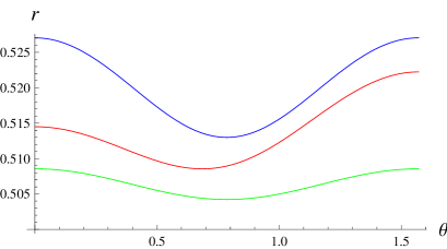
Figure 5.1: (Color online) The plots of the $\theta$ dependence of the exact solution $r(\theta)$ for the state (5.11). The top, middle and bottom lines represent the cases $(m=10,k=10),\;(m=12,k=18)$ and $(m=30,k=30)$, respectively.

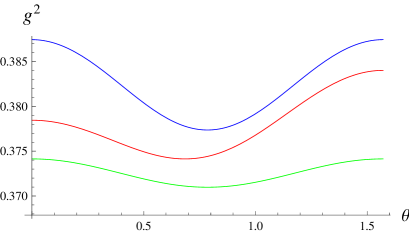
Figure 5.2: (Color online) The maximal product overlap function $\Lambda_{\max}^{2}(\theta)$ at different values of $m$ and $k$. The axes origin is put at the point $(0,1/e)$ to make it easer the comparison of the exact ant approximate solutions. The top, middle and bottom lines correspond to the values $(m=10,k=10),\;(m=12,k=18)$ and $(m=30,k=30)$, respectively.

As a consequence of Eq.(5.15) $\Lambda_{\max}^{2}$ is also almost constant and close to its lower bound $1/e$ [101]. Indeed, using approximations

$$\frac{1}{2^{m}}\left(1+\sqrt{1-\frac{a^{2}}{r^{2}}}\right)^{m}\approx e^{-ma^{2}/4r^{2}},\quad\frac{1}{2^{k}}\left(1+\sqrt{1-\frac{b^{2}}{r^{2}}}\right)^{k}\approx e^{-kb^{2}/4r^{2}}$$ (5.16)

one obtains

$$\Lambda_{\max}^{2}=\frac{1}{e}+O\left(\frac{1}{m}\right)+O\left(\frac{1}{k}\right).$$ (5.17)

The behavior of the maximal product overlap $\Lambda_{max}(\theta)$ given by Eqs. (5.6) and (5.13) is plotted in Fig.5.2, which shows that $\Delta\Lambda_{max}/\Lambda_{max}\sim 10^{-2}$ at $m,k\sim 10$. It is difficult if not impossible to observe such small deviations of the maximal product overlap in experiments and therefore approximate formulas (5.15) and (5.17) have a good accuracy when $N\geq 20$.

5.2.2 Three parameter W states

Consider now a three-parameter W state with $N=m+k+l$ qubits and coefficients

$$c_{1}=\cdots=c_{m}=a,\;c_{m+1}=\cdots=c_{m+k}=b,\;c_{m+k+1}=\cdots=c_{m+k+l}=c.$$ (5.18)

We will analyze the case $m,k,l\gg 1$. Then Eq. (5.5) can be rewritten as

$$m\sqrt{r^{2}-a^{2}}+k\sqrt{r^{2}-b^{2}}+l\sqrt{r^{2}-c^{2}}=(N-2)\,r.$$ (5.19)

From the normalization condition $ma^{2}+kb^{2}+lc^{2}=1$ it follows that $a^{2}\leq 1/m\ll 1$ and similarly $b^{2},c^{2}\ll 1$. On the other hand (5.19) shows that $r\sim 1$, and therefore we can expand the radicals in powers of $a^{2}/r^{2},\;b^{2}/r^{2}$ and $c^{2}/r^{2}$. Then

$$r^{2}=\frac{1}{4}+O\left(\frac{1}{m},\frac{1}{k},\frac{1}{l}\right).$$ (5.20)

Again we got the same answer for $r$, which means that for partitions with large number of qubits $r$ depends neither on $m,k,l$ nor on $a,b,c$. More precisely, $r$ depends only on the expression $ma^{2}+kb^{2}+lc^{2}=|\psi|^{2}$, which drops out owing to the normalization condition.

The equation (5.19) can be solved explicitly, but the resulting half-page answer is impractical and we will compare (5.20) with the numerical solution instead. For this purpose we use the parametrization

$$a=\sin\theta\cos\varphi/\sqrt{m},\;b=\sin\theta\sin\varphi/\sqrt{k},\;c=\cos\theta.$$

The behavior of the numerical solution $r(\theta)$ of Eq.(5.19) for various values $m,k,l$ and $\varphi$ is plotted in Fig.5.3. The graphics show that the approximate solution is in a perfect agreement with the numerical solution for $N\gg 1$.

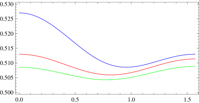
Figure 5.3: (Color online) The curves show the $\theta$ dependence of the function $r(\theta)$. The upper, middle and bottom curves represent the cases $(m=k=l=10,\varphi=\pi/4),\;(m=k=l=20,\varphi=5\pi/12)$ and $(m=10,k=20,l=30,\varphi=\pi/6)$, respectively.

In summary, in the symmetric region of highly entangled W states the maximal product overlap does not depend on state parameters when many qubits are involved. Consider a W state, where $n_{1},n_{2},...,n_{k}$ product vectors in the computational basis have coefficients $c_{1},c_{2},...,c_{k}$, respectively. Then $\Lambda_{max}$ does not depend on partition numbers $n_{i}$ or amplitudes $c_{i}$ and the approximate solution (5.15) with the maximal product overlap (5.17) quantifies the entanglement in high accuracy. For example, at $N\sim 10$ the accuracy is $\Delta\Lambda_{max}/\Lambda_{max}\sim 10^{-2}$. This approximation is true unless the condition $n_{i}\gg 1(i=1,2,...,k)$ is violated. What is happening if this condition is violated, is analyzed in the next section.

5.3 Asymmetric region of entanglement

In this section we consider three- and four-parameter W states in the asymmetric region and show that if one of coefficients exceeds the first critical value $r_{1}$, then $r$ is a rapidly increasing function and ranges from one-third to infinity when the maximal coefficient ranges from the first critical value to the second critical value.

5.3.1 Three-parameter W states

Consider now the case when $l=1$ in (5.18)

$$c_{1}=\cdots=c_{m}=a,\;c_{m+1}=\cdots=c_{m+k}=b,\;c_{m+k+1}=c.$$ (5.21)

If $c\ll 1$, then $c/r$ is small and $r$ is almost constant. This case is analyzed in the previous section and now we focus on the case when $c/r$ cannot be neglected. Then either $c\lesssim r_{1}$ or $r_{1}<c<r_{2}$.

When $c\lesssim r_{1}$ Eq.(5.5) takes the form

$$m\sqrt{r^{2}-a^{2}}+k\sqrt{r^{2}-b^{2}}+\sqrt{r^{2}-c^{2}}=(N-2)\,r.$$ (5.22)

The ratios $a/r$ and $b/r$ are small since $m,k\gg 1$. Hence we expand the radicals in powers of these ratios up to quadratic terms and solve the resulting equation. The answer is

$$r=\frac{1}{2}\frac{1-c^{2}}{\sqrt{1-2c^{2}}},\quad\sqrt{1-\frac{c^{2}}{r^{2}}}=\frac{1-3c^{2}}{1-c^{2}},\quad\max(a^{2},b^{2})<c^{2}\leq\frac{1}{3}.$$ (5.23)

It is reasonable that $r\to 1/2$ at $c\to 0$.

When $c\geq r_{1}$ Eq.(5.7) takes the form

$$m\sqrt{r^{2}-a^{2}}+k\sqrt{r^{2}-b^{2}}-\sqrt{r^{2}-c^{2}}=(N-2)\,r.$$ (5.24)

Its approximate solution is

$$r=\frac{1}{2}\frac{1-c^{2}}{\sqrt{1-2c^{2}}},\quad\sqrt{1-\frac{c^{2}}{r^{2}}}=\frac{3c^{2}-1}{1-c^{2}},\quad\frac{1}{3}<c^{2}<\frac{1}{2}.$$ (5.25)

As one would expect, $r\to\infty$ at $c^{2}\to 1/2$.

Surprisingly, both solutions (5.23) and (5.25) can be unified to a single solution as follows

$$r=\frac{1}{2}\frac{1-c^{2}}{\sqrt{1-2c^{2}}},\quad\max(a^{2},b^{2})<c^{2}<\frac{1}{2}.$$ (5.26)

The question at issue is when (5.26) gives a required accuracy in the asymmetric region $r_{1}<c<r_{2}$. We compare it with the numerical solutions of (5.22) and (5.24) for the values $(m=8,k=10,a/b=0.8,r_{1}^{2}\approx 0.34)$ in Fig.5.4, where the solid line is the plot of (5.26) and the dashed line is the numerical solution. Remarkably, the approximate solution is in a perfect agreement with the numerical one in the asymmetric region.

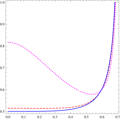
Figure 5.4: (Color online) Graphic illustrations of the function $r(c)$ for the three- and four-parameter W states. The solid curve is the approximate solution (5.26). The dashed curve is the joined numerical solution of Eqs. (5.22) and (5.24). All remaining coefficients are well away from the first critical value $(\approx 0.58)$ when $c$ varies within the range of definition in this case. Accordingly, the state is in the symmetric region when $0<c<0.58$ and in the asymmetric region when $0.58<c<0.707$. The dotted line is the numerical solution for the state (5.27). Now another coefficient may exceed the first critical value. Therefore there are two first critical values, for the last and the preceding coefficients, respectively. The first critical value for the next to last coefficient $c$ is $\approx 0.606$ and for the last coefficient $d$ is $\approx 0.59$ which is attained at $c=0.45657$. Thus the state is in the symmetric region when $0.45657<c<0.606$ and in the asymmetric region otherwise. Remarkably, the three curves coincide when $c>0.606$.

5.3.2 Four-parameter W states

However, there are W state that are outside the realm of the model sketched in the previous subsection. These are states with few (at most three) coefficients close to the first critical value $r_{1}\sim 1/\sqrt{3}$. In this case these coefficients are not small and the resulting $r$ should has a different behavior.

Notice, two coefficients cannot exceed the first critical value simultaneously. But we can construct W states whose coefficients depend on a free parameter in such a way that at one value of the free parameter the last coefficient exceeds the first critical value and at another value of the free parameter the preceding coefficient exceeds the first critical value. Below we construct an illustrative example of a such state and analyze its entanglement diameter.

An example is the 19-qubit four-parameter W state with coefficients

$$c_{1}=\cdots=c_{7}\equiv a,\;c_{8}=\cdots=c_{17}\equiv b,\;c_{18}\equiv c,\;c_{19}\equiv d.$$ (5.27)

For the normalized states we can use free parameters $\varphi,\;k$ and $c$ as follows

$$a^{2}=\frac{\cos^{2}\varphi}{7k}(1-c^{2}),\;b^{2}=\frac{\sin^{2}\varphi}{10k}(1-c^{2}),\;d^{2}=\frac{k-1}{k}(1-c^{2}).$$

Now we analyze the function $r(c)$ at $k=1.8,\varphi=\pi/4$.

1. The next to last coefficient $c$ coincides with its first critical value $r_{1}(c)$ at $c\approx 0.606$ , that is, the solution of the system

   $$7\sqrt{r_{1}^{2}-a^{2}}+10\sqrt{r_{1}^{2}-b^{2}}+\sqrt{r_{1}^{2}-d^{2}}=17r_{1}\;\,{\rm and}\;\,r_{1}=c$$

   is $r_{1}=c\approx 0.606$. Then $r(c)$ should range from $r_{1}(c)$ to infinity when $c$ ranges from $r_{1}(c)$ to 1/2 and should has a vertical asymptote at $c^{2}\to 1/2$.

2. The last coefficient $d$ coincides with its first critical value $r_{1}(d)$ at $d\approx 0.593$, that is, the solution of the system

   $$7\sqrt{r_{1}^{2}-a^{2}}+10\sqrt{r_{1}^{2}-b^{2}}+\sqrt{r_{1}^{2}-c^{2}}=17r_{1}\;\,{\rm and}\;\,r_{1}=d$$

   is $r_{1}=d\approx 0.593$. Note that at this point $c\approx 0.45657$. Then $r$ should increase when $d$ ranges from $r_{1}(d)$ to $d_{\max}$. But the maximum value of $d$ is less than the second critical value since $d_{\max}^{2}=d^{2}(c=0)=(k-1)/k=4/9<1/2$. Therefore $r$ should be bounded above in the interval $[r_{1}(d),d_{max}]$ and attain a maximum at $d_{max}$. As $d$ is a decreasing function on $c$, $r$ should attain a maximum at $c=0$ and then decrease when $c$ ranges from 0 to 0.45657.

3. The state is in the symmetric region when $d<r_{1}(d)$ and $c<r_{1}(c)$. Hence $r(c)$ should be minimal and nearly constant when $0.45657<c<0.606$.

The dotted line in Fig.5.4 represents the $c$ dependence of the function $r(c)$. It agrees completely with the above analyze.

The main point is that all the three curves coincide when $c>r_{1}(c)$. In the next section we will show that this is not accidental and the curves must coincide. In this context the equation (5.26) is a surprising result. The quantity $r$, as well as the maximal product overlap $\Lambda_{max}$, depends from $c$ only. The rest of the state parameters appear in (5.26) in the combination $|\psi|^{2}-c^{2}$ and drop out by the normalization condition!

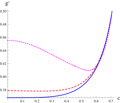
Figure 5.5: (Color online) The plots of the function $\Lambda_{max}(c)$. The solid line is the approximate solution (5.28), the dashed and dotted lines are the numerical solutions for the states (5.21) and (5.27), respectively. The curves may have different behaviors when $c_{N}<r_{1}$, but coincide when $c_{N}\geq r_{1}$.

Furthermore, we can derive an analytic expression for the maximal overlap. Using approximations (5.16) one obtains

$$\Lambda_{\max}^{2}(c)=(1-c^{2})e^{-(1-2c^{2})/(1-c^{2})}.$$ (5.28)

The behavior of the function $\Lambda_{max}(c)$ is shown in Fig.5.5. The solid line is the curve (5.28), the dashed curve is the numerical solution for the state (5.21) and the dotted line is the numerical computation for the state (5.27). They all coincide when $c>r_{1}(c)$.

For highly entangled states the maximal product overlap ranges from its lower to the upper bound when $c$ ranges from $r_{1}$ to $r_{2}$. On the other hand the Bloch vector ${\bm{b}}$ of $N$th qubit is collinear with axis $z$ and $b_{z}=1-2c^{2}$. Thus $\Lambda_{max}$ is a one-variable function on $b_{z}$ and one can vary the entanglement of the multiqubit W state by altering the Bloch vector of a single qubit. The remaining qubits should be present in order to create an entanglement, but their individual characteristics do not play any role within the domain $-1<b_{z}<1-2r_{1}^{2},N\gg 1$. These qubits are just spectators, they should appear in the W state, but have no influence on the entanglement of the state.

5.4 General case

The results of the previous sections are based on the fact that the entanglement diameter $r$ is bounded below. In the symmetric region it is rigidly bound by the following theorem.

Theorem 1. If $r$ is a solution of Eq.(5.5), then

$$\frac{1}{4}\leq r^{2}\leq\frac{1}{2}.$$ (5.29)

Proof. Note that

$$\frac{c_{i}^{2}}{r^{2}}=\left(1+\sqrt{1-\frac{c_{i}^{2}}{r^{2}}}\right)\left(1-\sqrt{1-\frac{c_{i}^{2}}{r^{2}}}\right)\leq 2\left(1-\sqrt{1-\frac{c_{i}^{2}}{r^{2}}}\right).$$

By summing over $i$ the above inequality and using (5.5) and the normalization condition one obtains

$$\frac{1}{r^{2}}\leq 2(n-n+2)=4.$$

Hence $r^{2}\geq 1/4$. Next, from $x\leq\sqrt{x}$ for $0\leq x\leq 1$ it follows that

$$\sum_{i=1}^{n}\left(1-\frac{c_{i}^{2}}{r^{2}}\right)\leq\sum_{i=1}^{n}\sqrt{1-\frac{c_{i}^{2}}{r^{2}}},\quad{\rm or}\quad n-\frac{1}{r^{2}}\leq n-2,$$

that is, $r^{2}<1/2$.

The inequalities (5.29) allow us to understand the behavior of $\Lambda_{max}$ of arbitrary N-qubit W states in the symmetric region. Indeed, in this region $c_{i}^{2}\sim 1/N$ and therefore $c_{i}^{2}/r^{2}\ll 1$. Then one can expand the radicals in (5.5) and obtain

$$N-\frac{1}{2r^{2}}\approx N-2,$$

which generalizes (5.5) and (5.6) to arbitrary W states with $c_{N}\ll 1$.

In Eq.(5.18) we have chosen equal coefficients in order to reduce the number of independent parameters and make it easier the analyze. Now Theorem 1 states that it is irrelevant whether some coefficients coincide. Decisive factor is that the coefficients $c_{i}$ are small($\sim 1/\sqrt{N}$). Then the ratios $c_{i}/r$ are small since $r$ is bounded below $(\sim 1/2)$ and we can keep first nonvanishing orders of these ratios. Surprisingly, all these ratios are combined in such a way that they yield the Euclidean norm of the state function and the final answer becomes independent on the state parameters as well as the number of particles involved.

In the asymmetric region the entanglement diameter $r$ should has a lower bound but has not an upper bound since $r\to\infty$ at $c_{2}\to r_{2}$. One may expect that the lower bound of $r$ in the asymmetric region coincides with the upper bound of $r$ in the symmetric region. But the following theorem shows that this is not the case.

Theorem 2. If $r$ is a solution of Eq.(5.7), then

$$r^{2}\geq\frac{1}{3}.$$ (5.30)

Proof. We use the same technique, namely

$$\frac{1}{r^{2}}=\sum_{i}^{N-1}\frac{c_{i}^{2}}{r^{2}}+\frac{c_{N}^{2}}{r^{2}}\leq\sum_{i}^{N-1}2\left(1-\sqrt{1-\frac{c_{i}^{2}}{r^{2}}}\right)+\frac{c_{N}^{2}}{r^{2}},$$

or

$$\frac{1}{r^{2}}\leq 2-2\sqrt{1-\frac{c_{N}^{2}}{r^{2}}}+\frac{c_{N}^{2}}{r^{2}}\leq 3\quad{\rm since}\quad c_{N}\leq r.$$

This bound, as well as bounds (5.29), is tight, for example, $r^{2}\to 1/3$ at $c^{2}\to 1/3$ in (5.26).

Theorem 2 explains why the asymmetric approximate solution (5.26) fits the numerical date more quickly ($N\sim 10$) than the symmetric one (5.15)($N\sim 20$). First, the lower bound of $r$ is greater in this case. Second, since $c_{N}$ is greater($c_{N}>r_{1}$) the remaining coefficients should be smaller due to the normalization condition. These two factors together make the ratio $c_{i}/r$ smaller. Hence the approximate solution should has a better agreement with the exact one. Aside from that, $r$ is a fast increasing function and goes to the infinity unlike to the symmetric case. Hence the values of the coefficients $c_{i}$ become irrelevant when $r\gg 1$.

In fact there is no W state in the asymmetric region that differs markedly from the above model when many qubits are involved. The following theorem completes the proof that in the asymmetric region the maximal product overlap is a one-variable function.

Theorem 3. If $c_{N}=r_{1}$, then

$$r_{1}^{2}=\frac{1}{3}+O(\frac{1}{N})$$ (5.31)

Proof. Note that on the boundary of the symmetric and asymmetric regions $r=r_{1}=c_{N}$ and therefore $r_{1}^{2}\geq 1/3$. Expanding the radicals in (5.3) in powers of $c_{i}^{2}/r_{1}^{2}$ one obtains

$$N-1-\frac{1-c_{N}^{2}}{2c_{N}^{2}}+O(\frac{1}{N})=N-2,$$

which gives (5.31).

Now we are ready to explain what is happening in the asymmetric region.

1. When many qubits $(N\gg 1)$ are involved the first critical value depends neither the number of qubits nor the state parameters and is a constant, $r_{1}\approx 1/\sqrt{3}$.

2. Regardless what is happening in the interval $0<c_{N}<r_{1}$ all functions $r(c)$ must converge to the point $r(1/\sqrt{3})\approx 1/\sqrt{3}$. This is the effect of the first critical value.

3. All functions $r(c)$ have the the same vertical asymptote, namely, $r(c)\to\infty$ at $c\to 1/\sqrt{2}$. This is the effect of the second critical value.

These statements together give no chance to differ markedly exact and approximate solutions in the asymmetric region. In conclusion, when $N\gg 1$, everywhere the maximal product overlap of W states is governed by the smallest $b_{z}$ among the $z$ components of the Bloch vectors. Using approximations

$$\frac{1}{2}\left(1+\sqrt{1-\frac{c_{i}^{2}}{r^{2}}}\right)\approx e^{-c_{i}^{2}/4r^{2}},\quad i=1,2,\cdots,N-1$$

and equations (5.9) and (5.26) one obtains

$$\Lambda_{\max}^{2}(N\gg 1)=\begin{cases}\enskip\frac{1+b_{z}}{2}\,e^{-\frac{2b_{z}}{1+b_{z}}},&{\rm if}\quad 0<b_{z}<\frac{1}{3}\cr\enskip\frac{1-b_{z}}{2},&{\rm if}\quad b_{z}<0\end{cases}$$ (5.32)

Graphic comparison of the interpolating formula and numerical computation of $\Lambda_{max}$ is shown in Fig. 5.6, where the $b_{z}$ dependence of $\Lambda_{max}$ is plotted for $N=10$. The solid and dashed lines represent the interpolating function (5.32) and numerical computation, respectively.

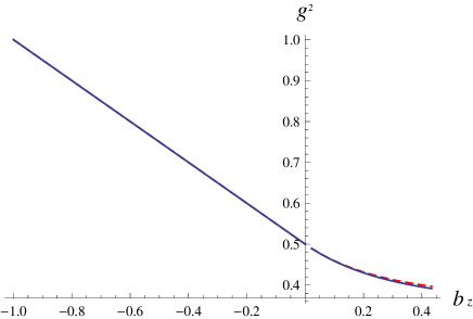
Figure 5.6: (Color online) The maximal product overlap $\Lambda_{max}$ as a function of $z$ component of the Bloch vector $b_{z}$. The solid line is the interpolating formula (5.32). The dashed line is the numerical computation for a 10-qubit W state.

We did not plotted numerical results for different states because different curves overlap and become indistinguishable. We failed to find the states for which the numerical results markedly differ from the plotted one provided $N\gg 1$ holds.

5.5 Discussion

The main result of this work is the formula (5.32). First, it shows that sometimes the characterization and manipulation of the entanglement of many qubit states is a simple task, while the case of few or several qubits is a complicated problem. Second, it states that when $N\gg 1$ the maximal product overlap of W states is universal in the asymmetric and slightly entangled regions and the only exceptions are W states in the symmetric region that are almost maximally entangled states. Then a question arises: Why do the maximal product overlaps of the different W states far apart from the exceptional points have the same behavior? Perhaps the reason is that these states are all W-class states. Classification of entangled states explains that pure states can be probabilistically converted to one another within the same class by stochastic local operations and classical communication [50, 84, 103]. And one can assume that large-scale systems within the same class have the feature, aside from the interconvertibility, that their entanglement is universal. An argument in favor of this assumption is that the geometric measure of entanglement [26], the relative entropy of entanglement [24] and the logarithmic global robustness [90] are related by bounding inequalities and, moreover, the relative entropy of entanglement is an upper bound to entanglement of distillation. Hence it is unlikely that these measures may exhibit contradicting results and each of them predicts its own and very different entanglement behavior of large-scale W-states. If this argument is true, then entanglement of large-scale states within the same class is universal. However, states from the different classes may exhibit different behaviors. By no means it is obvious, and probably not true, that the maximal product overlap of GHZ-class states should have a behavior similar to that of W states.

Another possible explanation is that the universality of the maximal overlap of large scale W states is the inherent feature of the geometric entanglement measure rather than the inherent feature of quantum states. If it is indeed the case, then a reasonable question is the following: do the exceptional points really exist or they are just the fabrication of the geometric entanglement measure? In this context the second exceptional point is a fundamental quantity. Indeed, there are states applicable for the perfect teleportation and dense coding and these states all should possess the same amount of entanglement. Hence there is an specific entanglement point(infinite entanglement diameter in the case of the geometric measure) that can be associated with the exceptional point. And one can assume that the second exceptional point is a property of quantum states rather than a property of the maximal product overlap. And how about the first exceptional point? Unfortunately, we do not know any strong arguments in favor of it. In order to clarify the existence or nonexistence of the first exceptional point, as well as the second exceptional point, one has to analyze another reliable entanglement measure, say relative entropy of entanglement [104], and see whether it possesses exceptional points.

Chapter 6 Non-strict inequality for Schmidt coefficients of three-qubit states

In this chapter we analyze generalized Schmidt decomposition for three-qubit states and establish a relation between those Schmidt coefficients [54].

Tripartite entanglement is a difficult subject for physicists. Essential results were obtained in this field [39, 48, 50, 58], but fundamental problems remain unsolved. Two of them are the main obstacles to understand tripartite entanglement so well as bipartite entanglement.

The first problem is the entanglement transformation problem. Its essence is the set of necessary and sufficient conditions for transforming a given pure tripartite state to another pure tripartite state by local operations and classical communication. This problem is solved for bipartite systems [56] and therefore the conditions for bipartite entanglement transformation based on majorization give a concise answer to the questions: among given states which ones are more/less entangled and which ones are incomparable? Unfortunately these problem is a puzzle in the case of tripartite systems.

The second problem, closely related to the first one, is the notion of maximally entangled states. This problem also is solved for bipartite systems and maximally entangled two-qubit states are the Einstein-Podolsky-Rosen state [15] and its local unitary(LU) equivalents known as Bell states [16]. However, there is no clear and unique definition of a maximally entangled state in multipartite settings. Consequently it is impossible to introduce operational entanglement measures based on optimal rates of conversion between arbitrary states and maximally entangled states [20, 21, 22].

For bipartite systems these problems have been solved with the help of the Schmidt decomposition [46, 47]. Therefore its generalization to multipartite states can solve difficult problems related to multipartite entanglement. This generalization for three qubits is done by Acín et al [48], where it is shown that an arbitrary pure state can be written as a linear combination of five product states. Independently, Carteret et al developed a method for such a generalization for pure states of arbitrary multipartite system, where the dimensions of the individual state spaces are finite but otherwise arbitrary [39]. The main idea of this method is the following. First one finds the product vector which gives maximal overlap with a given quantum state vector. Then one considers product vectors orthogonal to the first product vector and finds among them the product vector that gives maximal overlap with the state vector. Continuing in this way, one finds a set of orthogonal product states and presents the state function as a linear combination of these product vectors. Since the first product vector is a stationarity point, the resulting canonical form contains a minimal set of state parameters.

Just as in bipartite case, the largest coefficient of this canonical form is the maximal product overlap which is an increasing entanglement monotone [25]. Just as in bipartite case, the second largest coefficient is the maximal overlap over product states orthogonal to the nearest product state and so on. Additionally, this generalization of the Schmidt decomposition(GSD) gives insight into the nature of the maximally entangled three-qubit states [40] and is a good tool to extend Nielsen’s theorem and operational entanglement measures to multipartite cases. Hence we accept that the amplitudes of GSD proposed in [39] are multipartite Schmidt coefficients.

However, for a given quantum state the canonical form is not unique and the same state can have different canonical forms and therefore different sets of such amplitudes. The reason is that the stationarity equations defining stationarity points are nonlinear equations and in general have several solutions of different types. For instance, three-parameter W type states have four stationary points that create four equivalent canonical forms for the same W type state. This point is explained in detail in section III and now we focus on the question which of amplitude sets should be treated as Schmidt coefficients and which ones should be treated as insignificant mathematical solutions. A criterion should exist that can distinguish right Schmidt coefficients from false ones and we need such a criterion. It is unlikely that we can solve problems of three-qubit entanglement without knowledge of what quantities are the relevant entanglement parameters.

The canonical form whose largest coefficient is the maximal product overlap, as in bipartite case, presents GSD and others are irrelevant solutions of stationarity equations. Then our task is to single out the canonical form whose largest coefficient is the maximal product overlap and this requirement gives rise to a nontrivial relation between Schmidt coefficients of three-qubits. This situation differs from the bipartite case, where each set of positive numbers satisfying the normalization condition presents Schmidt coefficients of a some quantum state and its LU-equivalents. In contrary, in three-qubit case four positive and one complex coefficients satisfying the normalization condition are Schmidt coefficient if they satisfy an equality (derived in section V), otherwise they do not present relevant entanglement parameters at all. This is the main result of this work.

It is clear how do we single out the canonical form whose largest coefficient is the maximal product overlap. We should single out the closest product state of a given quantum state that gives a true maximum for overlap. Of course, we cannot find closest product states of generic three-qubit states because there is no method to solve generic stationarity equation so far. Hence to distinguish the true maximum from other stationary points we require that the second variation of the maximal product overlap is negative everywhere and this condition yields the desired inequality.

However, the derived non-strict inequality is a necessary but not a sufficient condition for specifying uniquely the Schmidt coefficients. It establishes an upper bound for the three middle coefficients and this upper bound is defined by the largest coefficient. But it does not give an upper bound for the last coefficient which also should have an upper bound conditioned by four previous coefficients. The existence of an upper bound for the last coefficient is clarified in section IV which means that an additional inequality is needed to distinguish clearly the right Schmidt coefficients from the false ones.

This chapter is organized as follows. In Sec. II we repeat the derivation of GSD for three-qubit systems. In Sec.III we present an illustrative example showing that the canonical form is not unique. In Sec. IV we compute the second variation of the maximal product overlap. In Sec.V we derive the non-strict inequality for three-qubit Schmidt coefficients and analyze particular cases. In Sec. VI we show that another inequality is needed to specify uniquely Schmidt coefficients. In Sec. VII we discuss our results.

6.1 Generalized Schmidt decomposition
for three-qubits

In this section we derive GSD for three-qubit pure states in detail since the derivation method is used in Sec.IV to compute the second variation of the maximal product overlap.

For a three-qubit pure state $|\psi\rangle$ the maximal product overlap $\lambda_{0}(\psi)$ is defined as

$$\Lambda_{max}\equiv\lambda_{0}(\psi)=\max|\langle u_{1}u_{2}u_{3}|\psi\rangle|,$$ (6.1)

where the maximum is over all tuples of vectors $|u_{k}\rangle$ with $\|u_{k}\|=1,(k=1,2,3)$. Note, hereafter the labels within each ket refer to qubits 1, 2 and 3 in that order.

To find the maximum of $\lambda_{0}(\psi)$ with constraints $\|u_{k}\|=1$ we form the auxiliary function $\Lambda$ given by

$$\Lambda=|\langle u_{1}u_{2}u_{3}|\psi\rangle|^{2}+\alpha_{1}(\langle u_{1}|u_{1}\rangle-1)+\alpha_{2}(\langle u_{2}|u_{2}\rangle-1)+\alpha_{3}(\langle u_{3}|u_{3}\rangle-1),$$ (6.2)

where the Lagrange multipliers $\alpha_{k}$ enforce unit nature of the local vectors $|u_{k}\rangle$.

Now we consider small variation of $|u_{k}\rangle$ and $\alpha_{k}$, that is $|u_{k}\rangle\to|u_{k}\rangle+|\delta u_{k}\rangle;\,\alpha_{k}\to\alpha_{k}+\delta\alpha_{k}$, and compute the resulting variation of $\Lambda$. Hereafter $\delta\Lambda$ and $\delta^{n}\Lambda$ mean the full and the $n$th variation of $\Lambda$, respectively.

First we consider the first variation and require that $\delta^{1}\Lambda=0$. Then the vanishing of the partial derivatives of $\Lambda$ with respect to the Lagrange multipliers $\alpha_{k}$ gives

$$\langle u_{1}|u_{1}\rangle-1=\langle u_{2}|u_{2}\rangle-1=\langle u_{3}|u_{3}\rangle-1=0,$$ (6.3)

which are constraints on the local states $|u_{i}\rangle$.

The vanishing of the partial derivatives of $\Lambda$ with respect to these local states gives

$$\left\langle\psi|u_{1}u_{2}u_{3}\right\rangle\left\langle u_{2}u_{3}|\psi\right\rangle+\alpha_{1}|u_{1}\rangle = 0$$

$$\left\langle\psi|u_{1}u_{2}u_{3}\right\rangle\left\langle u_{1}u_{3}|\psi\right\rangle+\alpha_{2}|u_{2}\rangle = 0$$ (6.4)

$$\left\langle\psi|u_{1}u_{2}u_{3}\right\rangle\left\langle u_{1}u_{2}|\psi\right\rangle+\alpha_{3}|u_{3}\rangle = 0$$

and their Hermitian conjugates. From (6.1) it follows that $\alpha_{1}=\alpha_{2}=\alpha_{3}=-\lambda_{0}^{2}$ and therefore we can adjust phases of $|u_{k}\rangle$ so that stationarity equations (6.1) become

$$\left\langle u_{2}u_{3}|\psi\right\rangle=\lambda_{0}|u_{1}\rangle,\quad\left\langle u_{1}u_{3}|\psi\right\rangle=\lambda_{0}|u_{2}\rangle,\quad\left\langle u_{1}u_{2}|\psi\right\rangle=\lambda_{0}|u_{3}\rangle.$$ (6.5)

In the case of three-qubit states these equations are sufficient to construct GSD as follows. For each single-qubit state $|u_{k}\rangle$ there is, up to an arbitrary phase, a unique single-qubit state $|v_{k}\rangle$ orthogonal to it. Then from (6.5) it follows that the product states

$$|u_{1}u_{2}v_{3}\rangle,\quad|u_{1}v_{2}u_{3}\rangle,\quad|v_{1}u_{2}u_{3}\rangle$$

are orthogonal to $|\psi\rangle$ and (6.5) can be written as

$$\left\langle u_{1}|\psi\right\rangle = \lambda_{0}|u_{2}u_{3}\rangle+\lambda_{1}|v_{2}v_{3}\rangle,$$

$$\left\langle u_{2}|\psi\right\rangle = \lambda_{0}|u_{1}u_{3}\rangle+\lambda_{2}|v_{1}v_{3}\rangle,$$ (6.6)

$$\left\langle u_{3}|\psi\right\rangle = \lambda_{0}|u_{1}u_{2}\rangle+\lambda_{3}|v_{1}v_{2}\rangle.$$

We choose the phases of $|v_{k}\rangle$ such that $\lambda_{1},\lambda_{2},\lambda_{3}\geq 0$. Note that after this choice the collective sign-flip of $|v_{k}\rangle$’s does not change anything and we will use this freedom in a little while.

The state $\psi$ can be written as a linear combination of five product states as follows

$$|\psi\rangle=\lambda_{0}|u_{1}u_{2}u_{3}\rangle+\lambda_{1}|u_{1}v_{2}v_{3}\rangle+\lambda_{2}|v_{1}u_{2}v_{3}\rangle+\lambda_{3}|v_{1}v_{2}u_{3}\rangle+\lambda_{4}|v_{1}v_{2}v_{3}\rangle,$$ (6.7)

where $\lambda_{4}$ is a complex number. It has two constraints, first $\lambda_{0}\geq|\lambda_{4}|$ and second $-\pi/2\leq{\rm Arg}(\lambda_{4})\leq\pi/2$, which can be achieved by the simultaneous change of the signs of the local states $|v_{k}\rangle$.

Sometimes one relabels $|u\rangle\to|0\rangle,\;|v\rangle\to|1\rangle$ for the simplicity. We leave (6.7) as is and refer to as GSD for three-qubits.

6.2 Illustrative example

In this section we show that for a given state $|\psi\rangle$ the canonical form (6.7) is not unique except rare cases and additional relations are needed to single out the Schmidt decomposition from the useless canonical forms.

Consider a three-parameter family of W type states [50] given by

$$|w(a,b,c)\rangle=a|100\rangle+b|010\rangle+c|001\rangle,$$ (6.8)

where parameters $a,b,c$ are all positive since their phases can be eliminated by appropriate LU transformations. Stationarity equations (6.5) of this state have three simple solutions and one special solution which exists if and only if parameters $a,b,c$ can form a triangle [38].

The three simple solutions are

$$|u_{1}(1)\rangle=|1\rangle,\quad|u_{2}(1)\rangle=|0\rangle,\quad|u_{3}(1)\rangle=|0\rangle,\quad\lambda_{0}(1) = a;$$ (6.9)

$$|u_{1}(2)\rangle=|0\rangle,\quad|u_{2}(2)\rangle=|1\rangle,\quad|u_{3}(2)\rangle=|0\rangle,\quad\lambda_{0}(2) = b;$$ (6.10)

$$|u_{1}(3)\rangle=|0\rangle,\quad|u_{2}(3)\rangle=|0\rangle,\quad|u_{3}(3)\rangle=|1\rangle,\quad\lambda_{0}(3) = c;$$ (6.11)

where numbers within brackets mark solutions.

The fourth nontrivial solution is

$$|u_{1}(4)\rangle = \frac{a\sqrt{2r_{a}}\,|0\rangle+\sqrt{r_{b}r_{c}}\,|1\rangle}{4S},\quad|u_{2}(4)\rangle\frac{b\sqrt{2r_{b}}\,|0\rangle+\sqrt{r_{a}r_{c}}\,|1\rangle}{4S}$$

$$|u_{3}(4)\rangle = \frac{c\sqrt{2r_{c}}\,|0\rangle+\sqrt{r_{a}r_{b}}\,|1\rangle}{4S},\quad\lambda_{0}(4)=\frac{abc}{2S}$$ (6.12)

where

$$r_{a}=b^{2}+c^{2}-a^{2},$$

$$r_{b}=a^{2}+c^{2}-b^{2},$$ (6.13)

$$r_{c}=a^{2}+b^{2}-c^{2}$$

and $S$ is the area of the triangle $(a,b,c)$.

At $r_{a}r_{b}r_{c}=0$ the special solution reduces to a trivial solution. Note that absolute values of these quantities $|r_{a}|,|r_{b}|,|r_{c}|$ are magnitudes of Bloch vectors of the first, second and third qubits, respectively and $r_{a}r_{b}r_{c}=0$ means that some of one-particle reduced densities is a multiple of the unit matrix. In other words, the states with a completely mixed subsystems appear at the edge of the special solution and viceversa.

These four solutions of (6.5) give the following four canonical forms for the state (6.8)

$$|w(a,b,c)\rangle =$$

$$\!\!\!\lambda_{0}(1)|u_{1}(1)u_{2}(1)u_{3}(1)\rangle+b|v_{1}(1)u_{2}(1)v_{3}(1)\rangle+c|v_{1}(1)v_{2}(1)u_{3}(1)\rangle;$$

$$|w(a,b,c)\rangle =$$

$$\!\!\!\lambda_{0}(2)|u_{1}(2)u_{2}(2)u_{3}(2)\rangle+c|u_{1}(2)u_{2}(2)u_{3}(2)\rangle+a|v_{1}(2)v_{2}(2)u_{3}(2)\rangle;$$

$$|w(a,b,c)\rangle =$$

$$\!\!\!\lambda_{0}(3)|u_{1}(3)u_{2}(3)u_{3}(3)\rangle+b|u_{1}(2)v_{2}(2)v_{3}(2)\rangle+a|v_{1}(3)u_{2}(3)v_{3}(3)\rangle;$$

$$|w(a,b,c)\rangle =$$

$$\!\!\!\!\!\lambda_{0}(4)|u_{1}(4)u_{2}(4)u_{3}(4)\rangle+i\frac{\sqrt{2r_{a}r_{b}r_{c}}}{4S}|v_{1}(4)v_{2}(4)v_{3}(4)\rangle+$$

$$\!\!\!\!\!\!\frac{ar_{a}}{4S}|u_{1}(4)v_{2}(4)v_{3}(4)\rangle+\frac{br_{b}}{4S}|v_{1}(4)u_{2}(4)v_{3}(4)\rangle+\frac{cr_{c}}{4S}|u_{1}(4)u_{2}(4)v_{3}(4)\rangle.$$

Now which of these canonical forms is a right decomposition?

It is easy to clarify this question in this particular case since we have all solutions of the stationarity equations (6.5) and can single out the one whose largest coefficient is the dominant eigenvalue of (6.5).

The answer is [38]:

1. if $r_{a}<0$ then only $\lambda_{0}(1)$ is the maximal eigenvalue of (6.5), but $\lambda_{0}(2)$, $\lambda_{0}(3)$, $\lambda_{0}(4)$ are not.

2. if $r_{b}<0$ then only $\lambda_{0}(2)$ is the maximal eigenvalue of (6.5), but $\lambda_{0}(1)$, $\lambda_{0}(3)$, $\lambda_{0}(4)$ are not.

3. if $r_{c}<0$ then only $\lambda_{0}(3)$ is the maximal eigenvalue of (6.5), but $\lambda_{0}(1)$, $\lambda_{0}(2)$, $\lambda_{0}(4)$ are not.

4. otherwise only $\lambda_{0}(4)$ is the maximal eigenvalue of (6.5), but $\lambda_{0}(1)$, $\lambda_{0}(2)$, $\lambda_{0}(3)$ are not.

However, we are unable to solve (6.5) for generic states and single out the maximal eigenvalue in this way. Also we are not forced to compare all eigenvalues of (6.5) to see whether the largest coefficient of a given decomposition is the maximal product overlap. We can just require that it is a truly maximum of the product overlap instead and obtain a criteria which shows whether the largest coefficient of a given canonical form is the maximal product overlap of the state. This will be done in next sections.

6.3 The second variation
of the maximal product overlap

In this section we compute the second variation of the maximal product overlap.

We compute it at stationary points to single out truly maximums and therefore we use the results coming from the vanishing of the first variation. Straightforward calculation gives

$$\delta^{2}\Lambda = \lambda_{0}^{2}\left|\left\langle\delta u_{1}|u_{1}\right\rangle+\left\langle\delta u_{2}|u_{2}\right\rangle+\left\langle\delta u_{3}|u_{3}\right\rangle\right|^{2}$$

$$- \lambda_{0}^{2}\left(\|\delta u_{1}\|^{2}+\|\delta u_{2}\|^{2}+\|\delta u_{3}\|^{2}\right)$$

$$+ \lambda_{0}^{2}\left(\left\langle\delta u_{1}|u_{1}\right\rangle\left\langle\delta u_{2}|u_{2}\right\rangle+\left\langle\delta u_{1}|u_{1}\right\rangle\left\langle\delta u_{3}|u_{3}\right\rangle+\left\langle\delta u_{2}|u_{2}\right\rangle\left\langle\delta u_{3}|u_{3}\right\rangle+{\rm cc}\right)$$

$$+ \lambda_{0}\big{(}\lambda_{3}\left\langle\delta u_{1}|v_{1}\right\rangle\left\langle\delta u_{2}|v_{2}\right\rangle+\lambda_{2}\left\langle\delta u_{1}|v_{1}\right\rangle\left\langle\delta u_{3}|v_{3}\right\rangle$$

$$+ \lambda_{1}\left\langle\delta u_{2}|v_{2}\right\rangle\left\langle\delta u_{3}|v_{3}\right\rangle+{\rm cc}\big{)}$$

$$+ \delta\alpha_{1}\delta||u_{1}||^{2}+\delta\alpha_{2}\delta||u_{2}||^{2}+\delta\alpha_{3}\delta||u_{3}||^{2},$$

where cc means complex conjugate.

Using the identity $\|\delta u_{k}\|^{2}\equiv\left|\left\langle\delta u_{k}|u_{k}\right\rangle\right|^{2}+\left|\left\langle\delta u_{k}|v_{k}\right\rangle\right|^{2}$ it can be rewritten as

$$\delta^{2}\Lambda = -\lambda_{0}^{2}\left(\left|\left\langle\delta u_{1}|v_{1}\right\rangle\right|^{2}+\left|\left\langle\delta u_{2}|v_{2}\right\rangle\right|^{2}+\left|\left\langle\delta u_{3}|v_{3}\right\rangle\right|^{2}\right)$$

$$+ \lambda_{0}\big{(}\lambda_{3}\left\langle\delta u_{1}|v_{1}\right\rangle\left\langle\delta u_{2}|v_{2}\right\rangle+\lambda_{2}\left\langle\delta u_{1}|v_{1}\right\rangle\left\langle\delta u_{3}|v_{3}\right\rangle$$

$$+ \lambda_{1}\left\langle\delta u_{2}|v_{2}\right\rangle\left\langle\delta u_{3}|v_{3}\right\rangle+{\rm cc}\big{)}$$

$$+ \lambda_{0}^{2}\left(\delta||u_{1}||^{2}\delta||u_{2}||^{2}+\delta||u_{1}||^{2}\delta||u_{3}||^{2})+\delta||u_{2}||^{2}\delta||u_{3}||^{2}\right)$$

$$+ \delta\alpha_{1}\delta||u_{1}||^{2}+\delta\alpha_{2}\delta||u_{2}||^{2}+\delta\alpha_{3}\delta||u_{3}||^{2}.$$

From (6.3) it follows that terms containing $\delta||u_{k}||^{2}$ vanish and the second variation takes the form

$$\delta^{2}\Lambda = -\lambda_{0}^{2}\left(\left|\left\langle\delta u_{1}|v_{1}\right\rangle\right|^{2}+\left|\left\langle\delta u_{2}|v_{2}\right\rangle\right|^{2}+\left|\left\langle\delta u_{3}|v_{3}\right\rangle\right|^{2}\right)$$

$$+ \lambda_{0}\big{(}\lambda_{3}\left\langle\delta u_{1}|v_{1}\right\rangle\left\langle\delta u_{2}|v_{2}\right\rangle+\lambda_{2}\left\langle\delta u_{1}|v_{1}\right\rangle\left\langle\delta u_{3}|v_{3}\right\rangle$$

$$+ \lambda_{1}\left\langle\delta u_{2}|v_{2}\right\rangle\left\langle\delta u_{3}|v_{3}\right\rangle+{\rm cc}\big{)}.$$

From $\left\langle\delta u_{i}|v_{i}\right\rangle\left\langle\delta u_{j}|v_{j}\right\rangle\leq|\left\langle\delta u_{i}|v_{i}\right\rangle\left\langle\delta u_{j}|v_{j}\right\rangle|$ it follows that

$$\delta^{2}\Lambda\leq-\lambda_{0}\sum_{i,j=1}^{3}|\left\langle\delta u_{i}|v_{i}\right\rangle||\left\langle\delta u_{j}|v_{j}\right\rangle|A_{ij},$$ (6.21)

where the real and symmetric matrix $A$ is given by

$$A=\begin{pmatrix}\lambda_{0}&-\lambda_{3}&-\lambda_{2}\\ -\lambda_{3}&\lambda_{0}&-\lambda_{1}\\ -\lambda_{2}&-\lambda_{1}&\lambda_{0}\end{pmatrix}.$$ (6.22)

Note that the inequality (6.21) can be saturated when vectors $|\delta u_{k}\rangle$ are all multiples of vectors $v_{k}$ and therefore (6.21) gives the least upper bound of $\delta^{2}\Lambda$.

6.4 A non-strict inequality
for the Schmidt coefficients

In this section we derive a non-strict inequality for the Schmidt coefficients.

The condition $\delta^{2}\Lambda\leq 0$ holds everywhere if and only if the matrix $A$ is positive which means that

$${\rm tr}(A)\geq 0,\quad({\rm tr}(A))^{2}-{\rm tr}(A^{2})\geq 0,\quad\det(A)\geq 0,$$ (6.23)

where tr and det mean the trace and the determinant of a matrix, respectively.

The first condition ${\rm tr}(A)=3\lambda_{0}>0$ is satisfied and does not give anything. Similarly, the second condition $({\rm tr}(A))^{2}-{\rm tr}(A^{2})=6\lambda_{0}^{2}-2(\lambda_{1}^{2}+\lambda_{2}^{2}+\lambda_{3}^{2})>0$ is a triviality since $\lambda_{0}$ is the largest coefficient. But the third condition $\det(A)\geq 0$ gives

$$\lambda_{0}^{2}\;\geq\;\lambda_{1}^{2}+\lambda_{2}^{2}+\lambda_{3}^{2}+2\;\frac{\lambda_{1}\lambda_{2}\lambda_{3}}{\lambda_{0}}.$$ (6.24)

This is a new and unexpected relation which says that nondiagonal coefficients all together are bounded above by the quantity depending only on the largest coefficient and therefore they should be small.

Let us consider some particular cases. First consider the case when some of nondiagonal coefficients, namely $\lambda_{1}$, vanishes. Then (6.24) reduces to the

$$\lambda_{0}^{2}\;\geq\;\lambda_{2}^{2}+\lambda_{3}^{2},\quad\lambda_{1}=0.$$ (6.25)

The solution (6.9) and the canonical form (6.2) present this case. This happens when a quantum state is a linear combination of three product states and its amplitudes in a computational basis satisfy (6.25). Then the largest amplitude is the largest Schmidt coefficient and GSD is achieved by a simple flipping of local states. Similarly, the solution (6.10) with the form (6.2) and solution (6.11) with the form (6.2) are the cases $\lambda_{2}=0$ and $\lambda_{3}=0$, respectively.

Conversely, when amplitudes of a three-term state in a computational basis do not satisfy (6.25) it appears a special solution (6.2) which creates a new factoizable basis. In this basis new amplitudes of the state given by (6.2) satisfy (6.24). Indeed,

$$4(abc)^{2}\geq(ar_{a})^{2}+(br_{b})^{2}+(cr_{c})^{2}+r_{a}r_{b}r_{c},$$ (6.26)

which can be checked using triangle inequalities. This means that if amplitudes of the state were not satisfying (6.24) in the initial basis from product states then it appears a special solution giving rise to a new basis from product states and in this final basis amplitudes do satisfy (6.24).

In conclusion, (6.24) clearly indicates whether a given canonical form is GSD or not and this is its main advantage.

Another particular case which we would like to elucidate is the following. We want to find a quantum state for which (6.24) is saturated and nondiagonal coefficients have the maximal value. We equate all nondiagonal coefficients for the simplicity and (6.24) reduces to

$$\lambda_{0}\;\geq\;2\lambda,\quad\lambda_{1}=\lambda_{2}=\lambda_{3}\equiv\lambda$$ (6.27)

and we are looking for the states with $\lambda_{0}=2\lambda$. The W state is a such state, this is easy to see by setting $a=b=c$ in (6.2). These substitutions yield

$$\lambda_{0}(W)=2\lambda(W)=\sqrt{2}|\lambda_{4}(W)|,$$ (6.28)

which shows that (6.24) is indeed a non-strict inequality and gives the least upper bound for the nondiagonal coefficients.

6.5 Missed inequality

In this section we show that another inequality is needed to specify uniquely the Schmidt coefficients of three-qubit states. To prove this statement let us assume the converse. Then (6.24) is a necessary and sufficient condition and GSD coefficients should satisfy only (6.24) and $\lambda_{0}\geq|\lambda_{4}|$. Consider symmetric states and put $\lambda_{1}=\lambda_{2}=\lambda_{3}=\lambda$ which yields $\lambda_{0}\geq 2\lambda$. Then it exists a state such that $\lambda_{0}=|\lambda_{4}|=2\lambda$ and its GSD is given by

$$|\psi_{contr}\rangle=\frac{1}{\sqrt{11}}\left(2|000\rangle+|011\rangle+|101\rangle+|110\rangle+2|111\rangle\right).$$ (6.29)

This is a wrong GSD. Indeed,

$$\lambda_{0}^{2}(wrong)=\frac{4}{11},$$

but it is shown in Ref.[40] that absolute minimum of $\lambda_{0}^{2}$ over three-qubit pure states is 4/9 and this minimum is reached at the W state. Hence no three qubit state exists for which $\lambda_{0}^{2}<4/9$. For the sake of clarity we present the maximal product overlap and nearest product state for the state (6.29)

$$\lambda_{0}^{2}(right)=\frac{14+3\sqrt{2}}{22},\;|u_{1}u_{2}u_{3}\rangle=(\cos\theta|0\rangle+\sin\theta|1\rangle)^{\otimes 3},\;\tan\theta=1+\sqrt{2},$$ (6.30)

which can be derived by usual maximization tools.

This example shows that conditions $\lambda_{0}\geq 2\lambda$ and $\lambda_{0}\geq|\lambda_{4}|$ are insufficient and another relation should exist and this new relation should give bounds for the last Schmidt coefficient. We know that when all nondiagonal coefficients vanish the upper bound is $|\lambda_{4}(\max)|=\lambda_{0}$(known as GHZ state) and when all nondiagonal elements are maximal given by (6.28) the upper bound is $|\lambda_{4}(\max)|=\lambda_{0}/\sqrt{2}$(at the W state). Hence for $|\lambda_{4}|$ it exists an upper bound depending on the remaining coefficients and this upper bound gives those particular bounds at GHZ and W states, respectively.

We can derive this upper in some simple cases, for instance, when $\lambda_{2}=\lambda_{3}=0$ and the state is

$$|\psi_{simple}\rangle=\lambda_{0}|000\rangle+\lambda_{1}|011\rangle+\lambda_{4}|111\rangle,$$ (6.31)

where $\lambda_{4}$ is positive as its phase is meaningless in this case.

The stationarity equations (6.5) for the state (6.31) have a relevant solution given by

$$|u_{1}\rangle=\frac{\lambda_{1}|0\rangle+\lambda_{4}|1\rangle}{\sqrt{\lambda_{1}^{2}+\lambda_{4}^{2}}},\quad|u_{2}\rangle=|1\rangle,\quad|u_{3}\rangle=|1\rangle,\quad\lambda_{0}^{\prime}=\sqrt{\lambda_{1}^{2}+\lambda_{4}^{2}}.$$ (6.32)

From this solution it follows that (6.31) is a right decomposition if and only if $\lambda_{0}\geq\lambda_{0}^{\prime}$, that is

$$\lambda_{0}^{2}\,\geq\lambda_{1}^{2}+\lambda_{4}^{2},\quad\lambda_{2}=\lambda_{3}=0.$$ (6.33)

This inequality gives the least upper bound for the last Schmidt coefficient when two nondiagonal coefficients vanish. Unfortunately the tools used in this work were unable to find the least upper bound of $|\lambda_{4}|$ for generic states.

6.6 Summary

The main result of this work is the inequality (6.24). Its role is to separate out three-qubit Schmidt coefficients from the set of four positive and one complex numbers. As is explained in above section, it is a necessary but not a sufficient condition and another inequality should exist to complete the task.

It is likely that the three nondiagonal elements together define bounds for the last Schmidt coefficients in the missed inequality. Then the nondiagonal coefficients are not just extra terms in GSD, but the ones which can show some important features of tripartite entanglement unknown so far.

Another application of the derived non-strict inequality is that it can give us a hint how do we extend Nielsen’s protocol or operational entanglement measures to three-qubit states. For instance, in bipartite case the protocol relies on inequalities quadratic on Schmidt coefficients. In three-qubit case such a theorem should include cubic relations as is evident from (6.24).

Chapter 7 Summary

In this chapter we list the main results of the thesis.

1. We have developed a method to derive algebraic equations for the geometric measure of entanglement of three-qubit pure states. Owing to it we have presented the first calculation of the geometric measure of entanglement in a wide range of three-qubit systems, including the general class of W states and states which are symmetric under the permutation of two qubits. Additionally, we have shown that the nearest separable states are not necessarily unique, and highly entangled states are surrounded by a one-parametric set of equally distant separable states.

2. We have derived an explicit expression for the geometric measure of entanglement for three-qubit states that are linear combinations of four orthogonal product states and thus have Schmidt rank 4. Any pure three-qubit state can be written in terms of five preassigned orthogonal product states via Schmidt decomposition. Thus the states discussed here are more general states compared to the well-known Greenberger–Horne–Zeilinger and W states that have less rank. In fact, just a single step is needed to compute analytically the geometric measure for five-parameter states and thereby to get the answer for arbitrary three-qubit states.

3. Using derived analytic expressions we have established that the geometric measure for three-qubit states has three different expressions depending on the range of definition in parameter space. Each expression of the measure has its own geometrically meaningful interpretation. The states that lie on joint surfaces separating different ranges of definition, designated as shared states, are quantum channels for perfect teleportation and dense coding. Hence we have found a criterion which shows whether or not a given state can be be applied as a dual quantum channel.

4. The Groverian measures are analytically computed in various types of three-qubit states and the final results are also expressed in terms of local-unitary invariant quantities in each type. Hence we use this relations to classify entangled regions of the Hilbert space as follows: in each region some of polynomial invariants are important and define uniquely Groverian measure of entanglement, while the remaining polynomial invariants are irrelevant. In this way we obtained six different entangled regions for three-qubit pure states.

5. We have developed a powerful method to compute analytically entanglement measures of multipartite systems. The method is based on duality which consists of two bijections. The first one creates a map between highly entangled n-qubit quantum states and n-dimensional unit vectors. The second one does the same between n-dimensional unit vectors and n-part product states. In this way we have obtained a double map or duality. The main advantage of the map is that, if one knows any of the three vectors, then one instantly finds the other two.

6. We have found the nearest product states for arbitrary generalized W states of n qubits, and shown that the nearest product state is essentially unique if the W state is highly entangled. It is specified by a unit vector in Euclidean n-dimensional space. We have used this duality between unit vectors and highly entangled W states to find the geometric measure of entanglement of such states. The duality map reveals two critical values for quantum state parameters. The first critical value separates symmetric and asymmetric entangled regions of highly entangled states, while the second one separates highly and slightly entangled states.

7. We have shown that when N $\gg 1$ the geometric entanglement measure of general N-qubit W states, except maximally entangled W states, is a one-variable function and depends only on the Bloch vector with the minimal z component. Hence one can prepare a W state with the required maximal product overlap by altering the Bloch vector of a single qubit. Also we have computed analytically the geometric measure of large-scale W states by describing these systems in terms of very few parameters. The final formula relates two quantities, namely the maximal product overlap and the Bloch vector, that can be easily estimated in experiments.

8. We have derived an interpolating formula for the geometric measure of entanglement even if neither the number of particles nor the most of state parameters are known. The importance of the interpolating formula in quantum information is threefold. First, it connects two quantities, namely the Bloch vector and maximal product overlap, that can be easily estimated in experiments. Second, it is an example of how we compute entanglement of a quantum state with many unknowns. Third, if the Bloch vector varies within the allowable domain then maximal product overlap ranges from its lower to its upper bounds. Then one can prepare the W state with the given maximal product overlap bringing into the position the Bloch vector.

9. We have derived a non-strict inequality between three-qubit Schmidt coefficients, where the largest coefficient defines the least upper bound for the three nondiagonal coefficients or, equivalently, the three nondiagonal coefficients together define the greatest lower bound for the largest coefficient. In addition, we have shown the existence of another inequality which should establish an upper bound for the remaining Schmidt coefficient. The role of the inequalities is to separate out three-qubit Schmidt coefficients from the set of four positive and one complex numbers. Another application of the derived non-strict inequality is that it can give us a hint how do we extend entanglement transforming protocols or operational entanglement measures to three-qubit states.

Appendix A Matrix ${\cal O}$

One can easily show that the elements of ${\cal O}$ defined in Eq.(2.12) are given by

$${\cal O}_{11}=\frac{1}{2}\left(u_{11}u_{22}^{*}+u_{11}^{*}u_{22}+u_{12}u_{21}^{*}+u_{12}^{*}u_{21}\right)$$ (A.1)

$${\cal O}_{22}=\frac{1}{2}\left(u_{11}u_{22}^{*}+u_{11}^{*}u_{22}-u_{12}u_{21}^{*}-u_{12}^{*}u_{21}\right)$$

$${\cal O}_{33}=|u_{11}|^{2}-|u_{12}|^{2}$$

$${\cal O}_{12}=\frac{i}{2}\left(u_{12}u_{21}^{*}+u_{11}u_{22}^{*}-u_{12}^{*}u_{21}-u_{11}^{*}u_{22}\right)$$

$${\cal O}_{21}=\frac{i}{2}\left(u_{12}u_{21}^{*}+u_{11}^{*}u_{22}-u_{12}^{*}u_{21}-u_{11}u_{22}^{*}\right)$$

$${\cal O}_{13}=u_{11}u_{12}^{*}+u_{11}^{*}u_{12}$$

$${\cal O}_{31}=u_{11}u_{21}^{*}+u_{11}^{*}u_{21}$$

$${\cal O}_{23}=-i\left(u_{11}u_{12}^{*}+u_{21}^{*}u_{22}\right)$$

$${\cal O}_{32}=i\left(u_{11}u_{21}^{*}+u_{12}^{*}u_{22}\right)$$

where $u_{ij}$ is element of the unitary matrix defined in Eq.(2.12). It is easy to prove ${\cal O}{\cal O}^{T}={\cal O}^{T}{\cal O}={\textsl{1\!\!1}}$, which indicates that ${\cal O}_{\alpha\beta}$ is an element of O(3).

Appendix B Bloch representation

If the density matrix associated from the pure state $|\psi\rangle$ in Eq.(2.18) is represented by Bloch form like Eq.(2.17), the explicit expressions for $\vec{v}_{i}$ are

$$\vec{v}_{1}=\left(\begin{array}[]{c}2\lambda_{0}\lambda_{1}\cos\varphi\\ 2\lambda_{0}\lambda_{1}\sin\varphi\\ \lambda_{0}^{2}-\lambda_{1}^{2}-\lambda_{2}^{2}-\lambda_{3}^{2}-\lambda_{4}^{2}\end{array}\right)\hskip 28.45274pt\vec{v}_{2}=\left(\begin{array}[]{c}2\lambda_{1}\lambda_{3}\cos\varphi+2\lambda_{2}\lambda_{4}\\ -2\lambda_{1}\lambda_{3}\sin\varphi\\ \lambda_{0}^{2}+\lambda_{1}^{2}+\lambda_{2}^{2}-\lambda_{3}^{2}-\lambda_{4}^{2}\end{array}\right)$$ (B.7)

$$\hskip 85.35826pt\vec{v}_{3}=\left(\begin{array}[]{c}2\lambda_{1}\lambda_{2}\cos\varphi+2\lambda_{3}\lambda_{4}\\ -2\lambda_{1}\lambda_{2}\sin\varphi\\ \lambda_{0}^{2}+\lambda_{1}^{2}-\lambda_{2}^{2}+\lambda_{3}^{2}-\lambda_{4}^{2}\end{array}\right)$$ (B.11)

and the components of $h^{(i)}$ are

$$h^{(1)}_{11}=2\lambda_{2}\lambda_{3}+2\lambda_{1}\lambda_{4}\cos\varphi,\hskip 28.45274pth^{(1)}_{22}=2\lambda_{2}\lambda_{3}-2\lambda_{1}\lambda_{4}\cos\varphi$$ (B.12)

$$h^{(1)}_{33}=\lambda_{0}^{2}+\lambda_{1}^{2}-\lambda_{2}^{2}-\lambda_{3}^{2}+\lambda_{4}^{2},\hskip 28.45274pth^{(1)}_{12}=h^{(1)}_{21}=-2\lambda_{1}\lambda_{4}\sin\varphi$$

$$h^{(1)}_{13}=-2\lambda_{2}\lambda_{4}+2\lambda_{1}\lambda_{3}\cos\varphi,\hskip 28.45274pth^{(1)}_{31}=-2\lambda_{3}\lambda_{4}+2\lambda_{1}\lambda_{2}\cos\varphi$$

$$h^{(1)}_{23}=-2\lambda_{1}\lambda_{3}\sin\varphi,\hskip 28.45274pth^{(1)}_{32}=-2\lambda_{1}\lambda_{2}\sin\varphi$$

$$h^{(2)}_{11}=-h^{(2)}_{22}=2\lambda_{0}\lambda_{2},\hskip 28.45274pth^{(2)}_{33}=\lambda_{0}^{2}-\lambda_{1}^{2}+\lambda_{2}^{2}-\lambda_{3}^{2}+\lambda_{4}^{2}$$

$$h^{(2)}_{12}=h^{(2)}_{21}=0,\hskip 28.45274pth^{(2)}_{13}=2\lambda_{0}\lambda_{1}\cos\varphi$$

$$h^{(2)}_{31}=-2\lambda_{3}\lambda_{4}-2\lambda_{1}\lambda_{2}\cos\varphi,\hskip 28.45274pth^{(2)}_{23}=2\lambda_{0}\lambda_{1}\sin\varphi$$

$$h^{(2)}_{32}=2\lambda_{1}\lambda_{2}\sin\varphi.$$

The matrix $h^{(3)}_{\alpha\beta}$ is obtained from $h^{(2)}_{\alpha\beta}$ by exchanging $\lambda_{2}$ with $\lambda_{3}$. The non-vanishing components of $g_{\alpha\beta\gamma}$ are

$$g_{111}=-g_{122}=-g_{212}=-g_{221}=2\lambda_{0}\lambda_{4}$$ (B.13)

$$g_{113}=-g_{223}=2\lambda_{0}\lambda_{3},\hskip 28.45274ptg_{131}=-g_{232}=2\lambda_{0}\lambda_{2}$$

$$g_{133}=2\lambda_{0}\lambda_{1}\cos\varphi,\hskip 28.45274ptg_{233}=2\lambda_{0}\lambda_{1}\sin\varphi$$

$$g_{312}=g_{321}=2\lambda_{1}\lambda_{4}\sin\varphi,\hskip 28.45274ptg_{311}=-2\lambda_{2}\lambda_{3}-2\lambda_{1}\lambda_{4}\cos\varphi$$

$$g_{313}=2\lambda_{2}\lambda_{4}-2\lambda_{1}\lambda_{3}\cos\varphi,\hskip 28.45274ptg_{322}=-2\lambda_{2}\lambda_{3}+2\lambda_{1}\lambda_{4}\cos\varphi$$

$$g_{323}=2\lambda_{1}\lambda_{3}\sin\varphi,\hskip 28.45274ptg_{331}=2\lambda_{3}\lambda_{4}-2\lambda_{1}\lambda_{2}\cos\varphi$$

$$g_{332}=2\lambda_{1}\lambda_{2}\sin\varphi,\hskip 28.45274ptg_{333}=\lambda_{0}^{2}-\lambda_{1}^{2}+\lambda_{2}^{2}+\lambda_{3}^{2}-\lambda_{4}^{2}.$$

Appendix C Geometrical interpretation of the duality

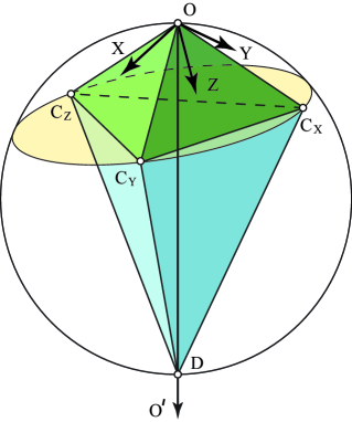
Figure C.1: (Color online) The geometrical interpretation of the duality for three-qubit W states. Mutually perpendicular bold lines $OX$, $OY$ and $OZ$ are coordinate axes and $\overrightarrow{OO^{\prime}}$ is an arbitrary direction. $OC_{X},\,OC_{Y}$ and $OC_{Z}$ are mirror images of the line $OO^{\prime}$ in respect to the three axes. The points $C_{X},\,C_{Y}$ and $C_{Z}$ are intersections of these lines with the sphere uniquely defined by the two conditions: its center lies on the line $OO^{\prime}$ and its diameter $OD\equiv r$ is the sum of the lateral sides of the upper pyramid (with the apex $O$ and base $C_{X}C_{Y}C_{Z}$). Now the direction cosines (and sines) of the vector $\overrightarrow{OD}$ are coefficients of the local states $|u_{i}\rangle$ in a computational basis. And the lateral sides of the lower pyramid (with the apex $D$ and base $C_{X}C_{Y}C_{Z}$) are the coefficients of a 3-qubit W-state in the same basis. Thus each direction singles out a product state and a W state and thereby establishes a correspondence among them.

The nearest product state $|u_{1}\rangle\otimes|u_{2}\rangle\otimes\cdots\otimes|u_{N}\rangle$ of the W state (5.1) can be parameterized as follows

$$|u_{k}\rangle=\sin\theta_{k}|0\rangle+\cos\theta_{k}|1\rangle,\,0\leq\theta_{k}\leq\frac{\pi}{2},\,k=1,2,...,N,$$ (B.1)

where

$$\cos^{2}\theta_{1}+\cos^{2}\theta_{2}+\cdots+\cos^{2}\theta_{N}=1.$$ (B.2)

Thus the angles $\cos\theta_{k}$ define a unit N-dimensional vector in Euclidean space. They satisfy the equalities

$$\frac{1}{r}\equiv\frac{\sin 2\theta_{1}}{c_{1}}=\frac{\sin 2\theta_{2}}{c_{2}}=\cdots=\frac{\sin 2\theta_{N}}{c_{N}}.$$ (B.3)

These equalities can be interpreted as trigonometric relations for the right triangles with hypotenuses $r$, angles $2\theta_{k}$, opposite legs $c_{k}$ and adjacent legs $\sqrt{r^{2}-c_{k}^{2}}$. If $2\theta_{k}>\pi/2$, then one takes the angle $\pi-2\theta_{k}$ instead. All of these triangles has the same hypotenuse $r$ and therefore can be circumscribed by a single sphere with the diameter $r$. The final picture represents two inscribed N-dimensional pyramids with a common base and lateral sides $c_{1},c_{2},...,c_{N}$ and $\sqrt{r^{2}-c_{1}^{2}},\sqrt{r^{2}-c_{2}^{2}},\sqrt{r^{2}-c_{N}^{2}}$, respectively. The case $N=3$ is illustrated in Fig.C.1.

Bibliography

- [1]
- [2] R. P. Feynman, Simulating Physics with Computers, Int. J. Theor. Physics 21, 467 (1982).
- [3] D. Deutsch, Quantum Theory, the Church-Turing Principle and the Universal Quantum Computer, Proc. R. Society Lond. A: 400, 97 (1985).
- [4] P. Shor, Algorithms for Quantum Computation: Discrete Logarithm and Factoring, Proc. 35th Annual Symposium on Foundations of Computer Science, 124-134 (1994).
- [5] L. M.K. Vandersypen, M. Steffen, G. Breyta, C. S. Yannoni, M. H. Sherwood, and I. L. Chuang, Experimental realization of Shor’s quantum factoring algorithm using nuclear magnetic resonance, Nature 414, 883 (2001).
- [6] A. K. Ekert, Quantum cryptography based on Bell s theorem, Phys. Rev. Lett 67, 661 (1991).
- [7] C. H. Bennett, F. Bessette, G. Brassard, L. Salvail and J. Smolin, Experimental Quantum Cryptography, J. Cryptology 5, 3 (1992).
- [8] C. H. Bennett and S. J. Wiesner, Communication via one- and two-particle operators on Einstein-Podolsky-Rosen states, Phys. Rev. Lett 69, 2881 (1992).
- [9] K. Mattle, H. Weinfurter, P. G. Kwiat and A. Zeilinger, Dense Coding in Experimental Quantum Communication, Phys. Rev. Lett. 76, 4656 (1996).
- [10] C. H. Bennett, G. Brassard, C. Crépeau, R. Jozsa, A. Peres, and W. K. Wootters, Teleporting an unknown quantum state via dual classical and Einstein-Podolsky-Rosen channels, Phys. Rev. Lett. 70, 1895 (1993).
- [11] D. Boschi, S. Branca, F. De Martini, L. Hardy and S. Popescu, Experimental Realization of Teleporting an Unknown Pure Quantum State via Dual Classical and Einstein-Podolsky-Rosen Channels, Phys. Rev. Lett. 80, 1121 (1998).
- [12] G. Vidal, Efficient Classical Simulation of Slightly Entangled Quantum Computations, Phys. Rev. Lett. 91 147902 (2003).
- [13] R. Jozsa and N. Linden, On the role of entanglement in quantum computational speed-up, Proc. R. Soc. Lond. A 459, 2011 (2003).
- [14] C. Negrevergne, T. S. Mahesh, C. A. Ryan, M. Ditty, F. Cyr-Racine, W. Power, N. Boulant, T. Havel, D. G. Cory, and R. Laflamme, Benchmarking Quantum Control Methods on a 12-Qubit System, Phys. Rev. Lett. 96, 170501 (2006).
- [15] A. Einstein, B. Podolsky, N. Rosen, Can quantum mechanical description of physical reality be considered complete?, Phys. Rev. 47, 777 (1935).
- [16] J. S. Bell, On the einstein-podolsky-rosen paradox, Physics (Long Island City, N.Y.) 1, 195 (1964).
- [17] R. F. Werner, Quantum states with Einstein-Podolsky-Rosen correlations admitting a hidden-variable model, Phys. Rev. A 40, 4277 (1989).
- [18] R. Horodecki, P. Horodecki, M. Horodecki, and K. Horodecki, Quantum entanglement, Rev. Mod. Phys. 81, 865 (2009).
- [19] M.B. Plenio and S. Virmani, An introduction to entanglement measures, Quant. Inf. Comp. 7, 1 (2007).
- [20] C. H. Bennett, H. J. Bernstein, S. Popescu, and B. Schumacher, Concentrating partial entanglement by local operations, Phys. Rev. A 53, 2046 (1996).
- [21] W. K. Wootters, Entanglement of Formation of an Arbitrary State of Two Qubits, Phys. Rev. Lett. 80, 2245 (1998).
- [22] C. H. Bennett, D. P. DiVincenzo, J. A. Smolin and W. K. Wootters, Mixed-state entanglement and quantum error correction, Phys. Rev. A 54, 3824(1996).
- [23] A. Shimony, Degree of entanglement, in D. M. Greenberg and A. Zeilinger (eds.), Fundamental problems in quantum theory: A conference held in honor of J. A. Wheeler, Ann. N. Y. Acad. Sci. 755 (1995) 675.
- [24] V. Vedral, M. B. Plenio, M. A. Rippin, and P. L. Knight, Quantifying Entanglement, Phys. Rev. Lett. 78, 2275 (1997).
- [25] H. Barnum and N. Linden, Monotones and Invariants for Multi-particle Quantum States, J. Phys. A: Math. Gen. 34, 6787 (2001).
- [26] T.-C. Wei and P. M. Goldbart, Geometric measure of entanglement and application to bipartite and multipartite quantum states, Phys. Rev. A 68 042307 (2003).
- [27] R. Werner and A. Holevo, Counterexample to an additivity conjecture for output purity of quantum channels, J. Math. Phys. 43, 4353 (2002).
- [28] L. K. Grover, Quantum Mechanics Helps in Searching for a Needle in a Haystack, Phys. Rev. Lett. 79, 325 (1997).
- [29] O. Biham, M. A. Nielsen and T. J. Osborne, Entanglement monotone derived from Grover’s algorithm, Phys. Rev. A 65, 062312 (2002).
- [30] J. J. Hilling and A. Sudbery, The geometric measure of multipartite entanglement and the singular values of a hypermatrix, J. Math. Phys. 51, 072102 (2010).
- [31] S. Tamaryan, A. Sudbery and L. Tamaryan, Duality and the geometric measure of entanglement of general multiqubit W states, Phys. Rev. A 81, 052319 (2010).
- [32] T.-C. Wei, M. Ericsson, P.M. Goldbart, and W.J. Munro, Connections between relative entropy of entanglement and geometric measure of entanglement, Quant. Inf. Comput. 4, 252 (2004).
- [33] D. Cavalcanti, Connecting the generalized robustness and the geometric measure of entanglement, Phys. Rev. A 73, 044302 (2006).
- [34] M. Hayashi, D. Markham, M. Murao, M. Owari, and S. Virmani, Bounds on Multipartite Entangled Orthogonal State Discrimination Using Local Operations and Classical Communication, Phys. Rev. Lett. 96, 040501 (2006).
- [35] O. Gühne, M. Reimpell and R.F. Werner, Estimating entanglement measures in experiments, Phys. Rev. Lett. 98, 110502 (2007).
- [36] R. Orús, Universal Geometric Entanglement Close to Quantum Phase Transitions, Phys. Rev. Lett. 100, 130502 (2008).
- [37] R. Orús, S. Dusuel, and J. Vidal, Equivalence of critical scaling laws for many-body entanglement in the Lipkin-Meshkov-Glick model, Phys. Rev. Lett. 101, 025701 (2008).
- [38] L. Tamaryan, D.K. Park and S. Tamaryan, Analytic Expressions for Geometric Measure of Three Qubit States, Phys. Rev. A 77, 022325 (2008).
- [39] H. A. Carteret, A. Higuchi, and A. Sudbery, Multipartite generalisation of the Schmidt decomposition, J. Math. Phys. 41, 7932 (2000).
- [40] S. Tamaryan, T.-C. Wei and D.K. Park, Maximally entangled three-qubit states via geometric measure of entanglement, Phys. Rev A 80, 052315 (2009).
- [41] E. Jung, M. R. Hwang, D. K. Park, L. Tamaryan and S. Tamaryan, Three-Qubit Groverian Measure, Quant. Inf. Comp. 8, 0925 (2008).
- [42] M. Hayashi, D. Markham, M. Murao, M. Owari, and S. Virmani, The geometric measure of entanglement for a symmetric pure state with positive amplitudes, J. Math. Phys. 50, 122104 (2009).
- [43] L. Tamaryan, D.K. Park, J.-W. Son, S. Tamaryan, Geometric Measure of Entanglement and Shared Quantum States, Phys. Rev. A 78, 032304 (2008).
- [44] T.-C. Wei and S. Severini, Matrix permanent and quantum entanglement of permutation invariant states, J. Math. Phys. 51, 092203 (2010).
- [45] R. Hübener, M. Kleinmann, T.-C. Wei, and O. Gühne, The geometric measure of entanglement for symmetric states, Phys. Rev. A 80, 032324 (2009).
- [46] E. Schmidt, Zur theorie der linearen und nichtlinearen integralgleighungen, Math. Ann. 63, 433 (1907).
- [47] A. Ekert and P. L. Knight, Entangled quantum systems and the Schmidt decomposition, Am. J. Phys. 63, 415 (1995).
- [48] A. Acín, A. Andrianov, L. Costa, E. Jané, J. I. Latorre and R. Tarrach, Generalized Schmidt Decomposition and Classification of Three-Quantum-Bit States, Phys. Rev. Lett. 85 (2000) 1560 [quant-ph/0003050].
- [49] D. Greenberger, M. Horne and A. Zeilinger, Going Beyond Bell’s Theorem, Phys. Today, August 1993, 24. arXiv:0712.0921[quant-ph]
- [50] W. Dür, G. Vidal and J. I. Cirac, Three qubits can be entangled in two inequivalent ways, Phys Rev. A 62, 062314 (2000).
- [51] E. Jung, M. R. Hwang, H. Kim, M. S. Kim, D. K. Park, J. W. Son and S. Tamaryan, Reduced state uniquely defines Groverian measure of original pure state, Phys. Rev. A 77, 062317 (2008).
- [52] L. Tamaryan, Z. Ohanyan and S. Tamaryan, Universal behavior of the geometric entanglement measure of many-qubit W states, Phys. Rev. A 82, 022309 (2010).
- [53] P. C. Hohenberg and B. I. Halperin, Theory of dynamic critical phenomena, Rev. Mod. Phys. 49, 435-479 (1977).
- [54] L. Tamaryan, Nonstrict inequality for Schmidt coefficients of three-qubit states, Phys. Rev. A 88, 042333 (2013).
- [55] A. Sudbery, On local invariance of pure three-qubit states, J. Phys. A 34 (2001) 643 [quant-ph/0001116].
- [56] M. A. Nielsen, Conditions for a Class of Entanglement Transformations, Phys. Rev. Lett. 83, 436 (1999).
- [57] N. Linden, S. Popescu and A. Sudbery, Nonlocal Parameters for Multiparticle Density Matrices, Phys. Rev. Lett. 83, 243 (1999).
- [58] V. Coffman, J. Kundu and W. K. Wootters, Distributed entanglement, Phys. Rev. A61, 052306 (2000).
- [59] N. Linden, S. Popescu and W. K. Wootters, Almost Every Pure State of Three Qubits Is Completely Determined by Its Two-Particle Reduced Density Matrices, Phys. Rev.Lett. 89, 207901 (2002).
- [60] B. Röthlisberger, J. Lehmann, D. S. Saraga, Ph. Traber and D. Loss, Highly Entangled Ground States in Tripartite Qubit Systems, Phys. Rev. Lett. 100, 100502 (2008), arXiv:0705.1710v1 [quant-ph].
- [61] Y. Shimoni, D. Shapira, and O. Biham, Entangled quantum states generated by Shor s factoring algorithm, Phys. Rev. A 72, 062308 (2005).
- [62] Y. Shimoni, D. Shapira, and O. Biham, Characterization of pure quantum states of multiple qubits using the Groverian entanglement measure, Phys. Rev. A 69, 062303 (2004).
- [63] P. Agrawal and A. Pati, Perfect teleportation and superdense coding with W states, Phys. Rev. A 74, 062320 (2006).
- [64] G. Vidal, D. Jonathan, and M. A. Nielsen, Approximate transformations and robust manipulation of bipartite pure-state entanglement, Phys. Rev. A 62, 012304 2000.
- [65] R. A. Bertlmann and Ph. Krammer, Geometric entanglement witnesses and bound entanglement, Phys. Rev. A 77, 024303 (2008).
- [66] G. Vidal, Entanglement monotones, J. Mod. Opt. 47 (2000) 355 [quant-ph/9807077].
- [67] M. B. Plenio and V. Vedral, Bounds on relative entropy of entanglement for multi-party systems, J. Phys. A 34 (2001) 6997 [quant-ph/0010080].
- [68] S. Hill and W. K. Wootters, Entanglement of a Pair of Quantum Bits, Phys. Rev. Lett. 78 (1997) 5022 [quant-ph/9703041].
- [69] Y. Most, Y. Shimoni and O. Biham, Formation of Multipartite Entanglement Using Random Quantum Gates, Phys. Rev. A 76 (2007) 022328, arXiv:0708.3481[quant-ph].
- [70] A. O. Pittenger and M. H. Rubin, The geometry of entanglement witnesses and local detection of entanglement, Phys. Rev. A 67, 012327 (2003) [quant-ph/0207024v1].
- [71] J. Eisert and H. J. Briegel, Schmidt measure as a tool for quantifying multiparticle entanglement, Phys. Rev. A 64 (2001) 022306 [quant-ph/0007081].
- [72] A. B. Zamolodchikov, “Irreversility” of the flux of the renormalization group in a 2D field theory, JETP Lett. 43 (1986) 730.
- [73] S. Tamaryan, , Completely mixed state is a critical point for three-qubit entanglement, Physics Letters A 375, 2224 2229(2011).
- [74] Y. Makhlin, Nonlocal properties of two-qubit gates and mixed states and optimization of quantum computations, Quant. Info. Proc. 1, 243-252 (2002), [quant-ph/0002045].
- [75] D. Shapira, Y. Shimoni and O. Biham, Groverian measure of entanglement for mixed states, Phys. Rev. A73, 044301 (2006).
- [76] L. Tamaryan, H. Kim, E. Jung, M.-R. Hwang, D.K. Park, and S. Tamaryan, Toward an understanding of entanglement for generalized n-qubit W-states, J. Phys. A: Math. Theor. 42, 475303 (2009).
- [77] C. H. Bennett, G. Brassard, S. Popescu, B. Schumacher, J. A. Smolin, and W. K. Wootters, Purification of Noisy Entanglement and Faithful Teleportation via Noisy Channels, Phys. Rev. Lett. 76, 722 (1996).
- [78] V. Vedral and M. Plenio, Entanglement measures and purification procedures, Phys. Rev. A 57, 1619 (1998).
- [79] C. H. Bennett, D. P. DiVincenzo, C. A. Fuchs, T. Mor, E. Rains, P. W. Shor, J. A. Smolin, and W. K. Wootters, Quantum nonlocality without entanglement, Phys. Rev. A 59, 1070 (1999).
- [80] K. Zyczkowski, P. Horodecki, A. Sanpera, and M. Lewenstein, Volume of the set of separable states, Phys. Rev. A 58, 883 (1998).
- [81] A. Harrow and M. Nielsen, Robustness of quantum gates in the presence of noise, Phys. Rev. A 68, 012308 (2003).
- [82] B. M. Terhal and K. G. H. Vollbrecht, Entanglement of Formation for Isotropic States, Phys. Rev. Lett. 85, 2625 (2000).
- [83] N. Linden, S. Popescu and A. Sudbery, Nonlocal Parameters for Multiparticle Density Matrices, Phys. Rev. Lett. 83, 243 (1999).
- [84] F. Verstraete, J. Dehaene, B. De Moor, and H. Verschelde, Four qubits can be entangled in nine different ways, Phys. Rev. A 65, 052112 (2002).
- [85] P. Parashar and S. Rana, N-qubit W states are determined by their bipartite marginals, Phys. Rev. A 80, 012319 (2009).
- [86] R. G. Unanyan, M. Fleischhauer, N. V. Vitanov, and K. Bergmann, Entanglement generation by adiabatic navigation in the space of symmetric multiparticle states, Phys. Rev. A 66, 042101 (2002).
- [87] M. Hayashi, D. Markham, M. Murao, M. Owari, and S. Virmani, Entanglement of multiparty-stabilizer, symmetric, and antisymmetric states, Phys. Rev. A, 77, 012104 (2008).
- [88] J. Martin, O. Giraud, P. A. Braun, D. Braun, and T. Bastin, Multiqubit symmetric states with high geometric entanglement, Phys. Rev. A 81, 062347 (2010).
- [89] H. Zhu, L. Chen, and M. Hayashi, Additivity and non-additivity of multipartite entanglement measures, New J. Phys. bf 12, 083002 (2010).
- [90] G. Vidal and R. Tarrach, Robustness of entanglement, Phys. Rev. A 59, 141(1999).
- [91] H. H. Adamyan and G. Yu. Kryuchkyan, Continuous-variable entanglement of phase-locked light beams, Phys. Rev. A 69, 053814 (2004).
- [92] R. G. Unanyan, C. Ionescu, M. Fleischhauer, Many-particle entanglement in the gaped antiferromagnetic Lipkin model, Phys. Rev. A 72, 022326 (2005).
- [93] S. S. Sharma and N. K. Sharma, Quantum coherences, K -way negativities and multipartite entanglement, Phys. Rev. A 77, 042117 (2008).
- [94] R. Hübener, M. Kleinmann, T.-C. Wei, C. G.-Guillen, and O. Gühne, Geometric measure of entanglement for symmetric states, Phys. Rev. A 80, 032324 (2009).
- [95] N. Linden, S. Popescu, and W. K. Wootters, Almost Every Pure State of Three Qubits Is Completely Determined by Its Two-Particle Reduced Density Matrices, Phys. Rev. Lett. 89, 207901 (2002).
- [96] A. Sen(De), U. Sen, M. Wiesniak, D. Kaszlikowski, and M. Zukowski, Multiqubit W states lead to stronger nonclassicality than Greenberger-Horne-Zeilinger states, Phys. Rev. A 68, 062306 (2003).
- [97] A. R. Usha Devi, R. Prabhu, and A. K. Rajagopal, Characterizing Multiparticle Entanglement in Symmetric N-Qubit States via Negativity of Covariance Matrices, Phys. Rev. Lett. 98, 060501 (2007).
- [98] X. Wang, Entanglement in the quantum Heisenberg XY model, Phys. Rev. A 64, 012313 (2001).
- [99] H. Mikami, Y. Li, K. Fukuoka, and T. Kobayashi, New High-Efficiency Source of a Three-Photon W State and its Full Characterization Using Quantum State Tomography, Phys. Rev. Lett. 95, 150404 (2005).
- [100] D. Gonta and S. Fritzsche, Multipartite W states for chains of atoms conveyed through an optical cavity, Phys. Rev. A 81, 022326 (2010).
- [101] Y. Shimoni, D. Shapira, and O. Biham, Characterization of pure quantum states of multiple qubits using the Groverian entanglement measure, Phys. Rev. A 69, 062303 (2004).
- [102] A. K. Pati, Minimum classical bit for remote preparation and measurement of a qubit, Phys. Rev. A 63, 014302 (2000).
- [103] T. Bastin, S. Krins, P. Mathonet, M. Godefroid, L. Lamata, and E. Solano, Operational Families of Entanglement Classes for Symmetric N-Qubit States, Phys. Rev. Lett. 103, 070503 (2009).
- [104] H. Kim, M.-R. Hwang, E. Jung, and D.K. Park, Difficulties in analytic computation for relative entropy of entanglement, Phys. Rev. A 81, 052325 (2010).