The Evolution of Dusty Debris Disks Around Solar Type Stars

Distribution of logR^′_HK

Distribution of Ages

Debris Disk Evolution

Dust Radii

Debris Disk Visualization

Debris Disk Visualization (cont’d)

Debris Disk Visualization (cont’d)

Distribution of Distances

Distribution of [Fe/H]

Planet Hosts

Li Evolution

Blackbody Degeneracy - HIP 90593

Abstract

We used chromospheric activity to determine the ages of 2,820 field stars.. We searched these stars for excess emission at 22 $\mu$m with the Wide-Field Infrared Survey Explorer. Such excess emission is indicative of a dusty debris disk around a star. We investigated how disk incidence trends with various stellar parameters, and how these parameters evolve with time. We found 22 $\mu$m excesses around 98 stars (a detection rate of 3.5$\%$). Seventy-four of these 98 excess sources are presented here for the first time. We also measured the abundance of lithium in 8 dusty stars in order to test our stellar age estimates.

1 INTRODUCTION

While most of the geological evidence about the evolution of our solar system has been erased by cataclysmic events, we can study the evolution of stellar systems like our own by observing circumstellar debris disks around solar-type (F, G, and K type) stars. Much work has been done to observe and characterize debris disks (e.g. Bryden et al. 2006), but it has been notoriously complicated to track the evolution of these disks. The root of the problem is the difficulty in determining stellar age. While the ages of clusters and associations can be determined by their bulk properties (i.e. HR diagrams), such techniques are not useful for isolated field stars.

Because of the difficulty of stellar age-dating, the study of debris disk evolution has been largely constrained to A-type stars (Su et al. 2006, Rieke et al. 2005). Since A-type stars evolve quickly on the main sequence, their ages can be estimated from stellar isochrones. Su et al. (2006) found that dust around A-type stars declines with age as t₀/t, where t₀=150 Myr.

Isochrone dating is not adequate for solar type stars, however, since they evolve slowly on the main sequence. It is important to extend the study of debris disk evolution to solar-type stars, since they offer the best evidence about the evolution of our own solar system. Chromospheric activity dating has a well-calibrated age relation, and carries smaller errors than isochrone dating (Mamajek $\&$ Hillenbrand 2008). We constructed a sample of 2,820 main-sequence field stars for which we have calculated age based on chromospheric activity. By using field stars, we created a sample with a smooth background age distribution. Thus, any dependence of debris disk incidence on stellar age should stand out.

The Wide-Field Infrared Survey Explorer (WISE; Wright et al. 2010) offers a unique opportunity to discover new circumstellar disks. WISE Band 4 (22 $\mu$m, hereafter W4) can trace infrared emission from the small (micron-sized) dust grains which dominate the emission from debris disks. Not only is WISE sensitive to 6 mJy (5$\sigma$) at 22 $\mu$m (Wright et al. 2010), but it also has the potential to catch debris disks around stars toward which other infrared observatories such as the Spitzer Space Telescope and Herschel Space Observatory may not have pointed. By pairing new age determination techniques with the all-sky coverage of WISE, we are able to provide new insight into the evolution of debris disks around solar-type stars.

Bryden et al. (2006) used Spitzer to search for IR excess emission around 127 F, G, and K type stars. They found seven stars with excess at 70 $\mu$m and only one star with excess at 24 $\mu$m. Trilling et al. (2008) followed by observing 184 F, G, and K type stars with Spitzer, finding seven with 24 $\mu$m excesses (an excess detection rate of 3.8$\%$). Spangler et al. (2001) observed $\sim$150 pre-main-sequence and main-sequence stars (mostly in clusters) with the Infrared Space Observatory (ISO). These were mostly young ($<$1 Gyr) F and G type stars. Thus, their detection rate will be higher than in an unbiased survey. They found 33 stars with evidence of IR excess (a detection rate of 22 $\%$). Koerner et al. 2010 used Spitzer to search for debris disks among 634 solar-type stars, finding a detection rate of 4.6$\%$ at 24 $\mu$m and 4.8$\%$ at 70 $\mu$m. In the present paper, we consider a sample of 2,820 stars with activity-determined ages which we examined with WISE at 22 $\mu$m, finding definite excesses around 98 stars (detection rate of 3.5$\%$).

In Section 2, we describe the process we used to determine whether or not an infrared excess was present. In Section 3, we elaborate on the age-determination method we used, and explain how we compiled our target list. In Section 4, we put our results in the context of current debris disk research. In Section 5, we describe any potential issues and errors associated with our findings.

2 IDENTIFYING AN IR EXCESS

Since most debris disks cannot be resolved, we depend on spectral energy distributions (SEDs) to identify IR excesses. SEDs were created with a fully automated fitting technique using theoretical models from Hauschildt et al. (1999) to predict stellar photospheric fluxes. The SEDs were generated using available photometry from Hipparcos (Perryman et al. 1997), Tycho-2 (Hog et al. 2000), 2MASS (Cutri et al. 2003), WISE (Cutri et al. 2012), and (when available) IRAS (Helou & Walker 1988). Stellar radii and effective temperatures are treated as free parameters to fit the observed fluxes (B, V, J, H, and K) with a $\chi$² minimization method. We chose not to fit the photosphere to the W1, W2, or W3 points due to saturation limits in the WISE data and the possibility of an excess at W3.

To characterize the IR excess (or lack thereof) in WISE, we concentrated on the W4 data (22 $\mu$m). The WISE data release provides the W4 flux density in magnitude units. We converted these magnitudes to flux densities in Jy using published WISE zero points. Using the photospheric fluxes predicted by the $\chi$² fit, we defined a parameter SNR:

$$SNR=\frac{W4[Jy]-W4_{phot}[Jy]}{N4[Jy]}$$ (1)

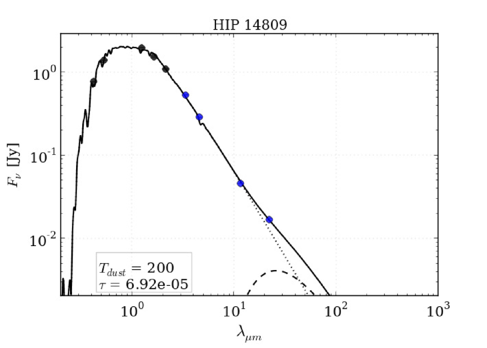
Figure 1: This is an SED for HIP 14809 - one of our debris disk candidates. Black dots represent data from Hipparcos and 2MASS catalogs (at B, V, J, H, and K bands). The blue dots represent WISE data in four bands (3.4, 4.6, 11 and 22 $\mu$m).This star represents the minimum amount of dust (amount of flux above the photosphere) which we felt comfortable characterizing as a debris disk.

where N4 is the noise (error) associated with each W4 measurement and W4_phot is the predicted 22 $\mu$m photospheric value. We choose to define a candidate excess source as one for which SNR$>$5. This constitutes a 5$\sigma$ detection. These candidate excess sources were double-checked visually to make sure that the calculated excess was not due to a bad photospheric fit. A blackbody was then fit to the apparent IR excess. When available, we used supplementary data from Spitzer and Herschel to better constrain the dust temperature and fractional IR luminosity. These data were downloaded from the NASA/IPAC Infrared Science Archive website (irsa.ipac.caltech.edu). Relevant data are found in Table 3. One SED representative of our sample is shown in Figure 1.

Zuckerman et al. (2011) found that Hauschildt photopsheric models underpredicted the flux at 22 $\mu$m by $\sim$3$\%$. We used a subset of stars from Jenkins et al. (2011) - a sample of stars with known chromospheric activity - to test the Hauschildt models. Of the 868 stars in the Jenkins sample, we used 230 stars which had SNR between -1 and 1, and which had W2 fluxes $<$1 Jy (to avoid the saturation limit at 2 Jy). We used this sample of 230 stars to compare two different photosphere models - one from Hauschildt et al. (1999), and the second a linear fit to W1, W2, and W3. In the end, we chose to define SNR using the “corrected” photospheric value (W4_phot*1.03).

Finally, the data products from WISE were individually inspected to make sure that there were no contaminating sources which could be mimicking an excess (such as a binary companion or a background galaxy). The FWHM of the PSFs for the different WISE bands are: W1(3.4 $\mu$m): 6.08$\arcsec$ ; W2(4.6 $\mu$m): 6.84$\arcsec$ ; W3(11 $\mu$m): 7.36$\arcsec$ ; W4(22 $\mu$m): 11.99$\arcsec$. Since we are considering excess in the W4 band, we use the FWHM of the PSF in that band as the contamination radius; if a point-like secondary source were found within 24$\arcsec$ (2$\times$FWHM_W4) of the target, we considered that star to be “contaminated” and it was no longer considered to be a candidate excess source. We allowed more room for extended nearby sources such as background galaxies. In the case of a nearby extended source, we define a contamination radius to be from the center of the contaminating galaxy to the center of the target in question, and set that radius at 1$\arcmin$. Furthermore, there were several cases in which an excess was seen at W4 in the SED, but no star is apparent in the WISE data product. These stars were considered non-detections. If none of the aforementioned issues were encountered, the data product is considered to be “clean.”

We also considered the possibility of an unseen background galaxy contaminating our W4 excess sources. Given that the WISE data products were checked for nearby sources, any remaining contaminating source would have to lie within the 6$\arcsec$ beam of the W4 band. Kennedy & Wyatt (2012) predict 0.06 spurious sources in their WISE 468 targets (a contamination rate of $\sim$0.01$\%$). Therefore, for our 2,820 targets, we would expect 0.36 spurious detections due to contamination by unseen background galaxies.

3 THE STELLAR SAMPLE

3.1 Chromospheric Activity as an Age Indicator

Stars with a deep convective zone (CZ) experience differential rotation which heats the CZ and ionizes the material in it. As this ionized material rotates, it enhances pre-existing weak magnetic fields. The strengthened magnetic field magnetizes material in the stellar wind as it leaves the system. This causes the outflowing material to rotate, resulting in a net loss of angular momentum. Over time, the star will spin-down which, in turn, reduces its magnetic activity. Thus as a star ages, it will spin down and its magnetic activity will weaken in a predictable way (Skumanich 1972, Barnes 2003)

The magnetic activity can be measured by looking at the collisonally-dominated Ca II H$\&$K absorption lines at $\sim$3900Å. In these lines, the photosphere of the star is suppressed by absorption, and we can see the emission cores due to magnetic heating of the chromosphere. Mamajek & Hillenbrand (2008) - hereafter MH08 - provide us with a cluster-calibrated relationship between chromospheric activity and age:

$$log(t)=-38.053-17.912(logR^{\prime}_{HK})-1.6675(logR^{\prime}_{HK})^{2}$$ (2)

where R^′_HK is a parameter measuring the strength of the Ca II H$\&$K emission core and t is age in years. This relation is only valid (calibrated) if -5.1$<$logR^′_HK$<$-4.0. Typical errors in age associated with this method are $\sim$60$\%$ (MH08). For some stars, there may be an additional uncertainty due to the long-period ($\sim$10 year) magnetic variations due to the stellar cycle. This is discussed further in Section 5.2.

In addition to an activity-age relation, MH08 suggests that an activity-rotation-age calculation can be used which, when used to calculate the ages of stars in binaries and open clusters, resulted in lower errors. Also, the activity-rotation-age relation takes the mass of the star (parameterized by the (B-V) color) into account.This calculation requires that the chromospheric activity index is first used to calculate the Rossby number (Noyes et al. 1984), which can then be used to calculate a rotation period. This period is then fed into a cluster-calibrated rotation-age (“gyrochronology”) relation:

$$P(B-V,t)=a[B-V_{0}-c]^{b}t^{n}$$ (3)

where MH08 found that a=0.407, b=0.325, c=0.495, and n=0.556 for a rotation period P in days and age t in Myr ((B-V)₀ is the de-reddened color). These constants were determined by fitting the rotation-age equation to clusters with known ages (up to the age of the Hyades - 625 Myr). It is valid for stars with 0.495$<$(B-V)₀$<$1.4. The combined activity-rotation-age relation was calibrated to clusters up to 625 Myr, field binaries up to $\sim$10 Gyr, and field stars up to $\sim$15 Gyr. By comparing the calculated ages of field binaries, MH08 were able to quote an average error of 15$\%$ in t. We present both the age calculated directly from the rotation-age relation of MH08 (Age_RHK) and the age calculated by using the Rossby number and the rotation-age relation (Age_ROT). All of our statistics were calculated using the latter.

In total, we cataloged WISE data for 2,820 stars with known chromospheric activity ages from 4 sources (Pace 2013 (1,251 stars); Jenkins et al. 2011 (596 stars); Isaacson $\&$ Fischer 2010 (854 stars); Wright et al. 2004 (119 stars)). When we found an overlap between these four sources, we preferentially took chromospheric data from the most recent publication.

3.2 Pace 2013

Pace (2013) collected a sample of 1,741 field stars with ages derived from stellar isochrones from the Geneva Copenhagen survey of the solar neighborhood. The goal was to constrain the age range in which chromospheric activity is a reliable age-determination tool. Of the 1,741 stars in the Pace (2013) sample, 1,251 stars have log(R^′_HK) in the appropriate range for the chromospheric activity relation from MH08 (-5.1$<$log(R^′_HK)$<$-4.0). After examining the SEDs, we found that 132 showed evidence of some excess. Of those, 42 have clean WISE data products. Of those 42 debris disks, 27 are previously unreported in the literature.

3.3 Jenkins et al. 2011

Jenkins et al. (2011) assembled a catalog of 890 stars with chromospheric emission measured with an echelle spectrograph. Their purpose was to calibrate their measured S-index to the Mount Wilson S-index, thus allowing them to derive a value for log(R^′_HK)for their sample. Of the 890 stars in the Jenkins et al. sample, 93 are also in the Pace (2013) sample. Of the 797 remaining stars, 596 have R^′_HK values in the appropriate range for our chromospheric activity relation. Of those 596, 33 have excesses in W4 and clean WISE data products. Of those, 30 are presented here for the first time.

3.4 Isaacson & Fischer 2010

Isaacson & Fischer (2010) collected spectral data for over 2,600 stars. Their goal was to determine if the “jitter” in their chromospheric activity measurements was due to the presence of a planetary system. Of the 2,647 stars in the Isaacson & Fischer (2010) sample, 420 are also either in the Pace (2013) sample or the Jenkins et al. (2011) sample. Of the remaining 2,227 stars, 854 are on the main sequence (according to SIMBAD) and have R^′_HK values in the appropriate range. Of the 854 stars we examined, 20 have W4 excesses and clean WISE data products. Of that subsample, 14 have no previous mention in the literature.

3.5 Wright et al. 2004

Wright et al. (2004) constructed a sample of over 1,200 F, G, K, and M type stars with chromospheric activity measurements derived from 18,000 spectra from Lick and Keck Observatories. Of the 1,204 stars in the Wright et al. (2004) sample, 119 are unique targets with R^′_HK in the appropriate range. Three stars have evidence of an IR excess at W4 and clean data products. Of those 3 stars, all are presented here for the first time.

4 DISCUSSION

4.1 Comparison to Protoplanetary Disks

The following discussion is taken largely from the Annual Review article by Wyatt (2008): The IR excess seen in debris disks differs significantly from that seen in protoplanetary disks. The most obvious difference is that protoplanetary disks consist largely of gas and sub-micron sized dust grains. These grains radiate very efficiently (due to their high surface area-volume ratio). Thus the fractional IR luminosities ($\tau$) seen in protoplanetary disks are several orders of magnitude higher than those seen in debris disks and higher yet compared to the Sun’s Kuiper Belt (KB)($\tau$_proto$\sim$10^-2, $\tau$_debris$\sim$10^-5, $\tau$_KB$\sim$10^-7). In addition to their higher IR luminosities, protoplanetary disks also have shorter lifetimes than debris disks. Most protoplanetary disks are completely dispersed $\sim$10 Myr after their formation due to mass loss and gas accretion onto the star (Wyatt 2008). Thus the circumstellar disks we see around $>$10 Myr stars must be second generation (Zuckerman 2001).

4.2 Models of Dust Production

The dust observed in debris disks is thought to have formed from a collisional cascade in the planetary disk. The generally accepted model of dust formation is as follows: Once the gas in the disk has been dispersed, rocky planetesimals can begin growing. At first, the disk experiences runaway growth as larger objects grow at faster rates due to gravitational focusing. Once objects reach $\sim$1000 km in size, they undergo oligarchic growth (Wyatt 2008). In this phase, a few large planetesimals clean out the small ($<$100 km) bodies in their neighborhood, and grow slowly into protoplanet-sized objects. At this stage, the large objects in the forming planetary system can dynamically stir the leftover small objects. These small objects will eventually be given enough of a velocity kick for the resulting collisions between small bodies to be destructive. The cold dust that we see around stars with ages $>$10 Myr is likely the result of these collisions.

4.3 Models of Dust Removal

Dust can be removed from the system in several ways. The most effective mechanism is due to radiative forces from the star. Once collisions between intermediate ($<$100km) sized bodies begins, a collisional cascade is triggered. Two bodies collide to create a population of smaller bodies, which collide with each other to create even smaller bodies, and so on until the debris reaches the blow-out radius. At this point, the dust can be ejected from the system by radiative forces. Dust can also be destroyed by spiraling toward the star as a result of Poynting-Robertson drag and ultimately being vaporized. Small particles can also be carried out by a strong stellar wind. However, since the dust collision timescale for observed debris disks is much smaller than the timescale for Poynting-Robsertson drag, most dust loss is “collision dominated.” (Zuckerman 2001).

4.4 Observations

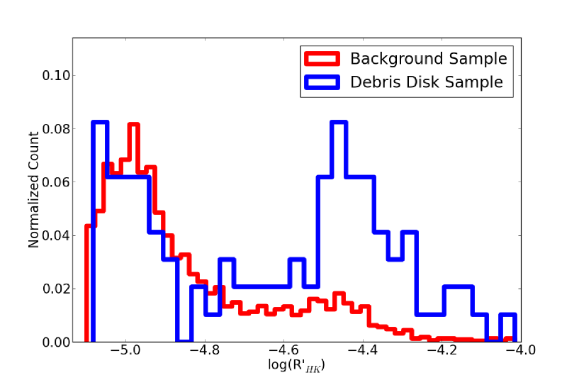
Figure 2: The distribution of stars as a function of their chromospheric activity parameter. It is clear that as the background sample (which includes the debris disk stars) decreases toward higher values of logR_HK (more active stars), the sample of debris disks does not. In fact, the distribution of debris disks appears to be somewhat bimodal.

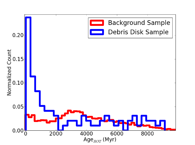
Figure 3: The distribution of stars as a function of stellar age, as determined from their chromospheric activity. While the background sample (which includes debris disks stars) has a smooth distribution of ages, there is a clear peak in the distribution of debris disks at younger ages.

We examined the WISE fluxes of 2,820 stars with chromospheric activity measurements. Of those, 98 have excesses at 22 $\mu$m (3.5$\%$). This detection rate agrees with the rate reported by Trilling et al. (2008) for 24$\mu$m excesses around 184 FGK stars (3.8$\%$). The ages of our debris disks range from 24 Myr to 9.1 Gyr, with an average of 2.7 Gyr. The debris disk parameters are found in Table 1, and the associated WISE data are found in Table 2. In Figure 2, we display the distribution of sample stars and debris disk stars as a function of chromospheric activity. We see the expected distribution of stars, with most of our sample being inactive (log(R^′_HK)$<$-4.8) and a hint of the Vaughan-Preston gap at intermediate activity levels (Vaughan & Preston 1980). It is clear that, relative to the background sample, debris disks are found preferentially around active stars. This is expected, since more active stars tend to also be younger. The distribution of the sample as a function of age is shown in Figure 3 and indeed, we see that debris disks are found preferentially around younger stars. By fitting a logarithmic decline to our histogram of debris disk ages, we find that the number of debris disks declines as e^t0/t where t₀$\sim$175 Myr (Figure 4). This is similar to the results from Su et al. 2006 who found that t₀$\sim$150 Myr.

We examined the evolution of the infrared luminosity fraction $\tau$ (=L_IR/L_bol) with age, where $\tau$ is determined from the following formula:

$$\tau=\frac{(\nu F_{\nu})_{peak,dust}}{(\nu F_{\nu})_{peak,star}}$$ (4)

where R_star and T_star are determined by the best-fit photospheric SED, T_dust is determined by the best-fit blackbody to the IR excess, and R_dust is determined from the equation:

$$R_{dust}=\frac{R_{star}}{2}(\frac{T_{star}}{T_{dust}})^{2}$$ (5)

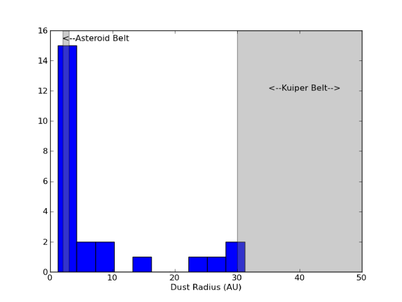
Figure 5: This figure shows a histogram of dust radii for systems with dust blackbodies fit to more than one mid-IR data point. The locations of the Asteroid Belt and Kuiper Belt of the Solar System are shown for comparison, along with the orbits of the 4 giant planets.

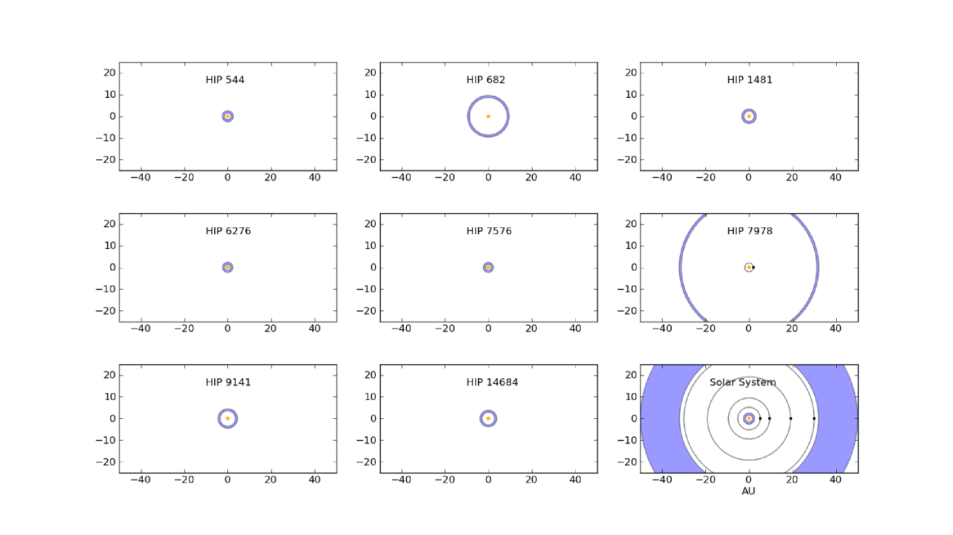
Figure 6: This figure is a visualization of debris disks in systems with well determined dust radii. Note that the thickness of the dust rings is artificially added. Two stars are previously known planet hosts (HIP 7978 and HIP 118319).

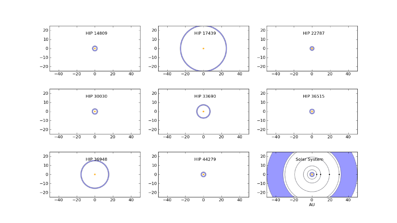
Figure 7: Same as Figure 6.

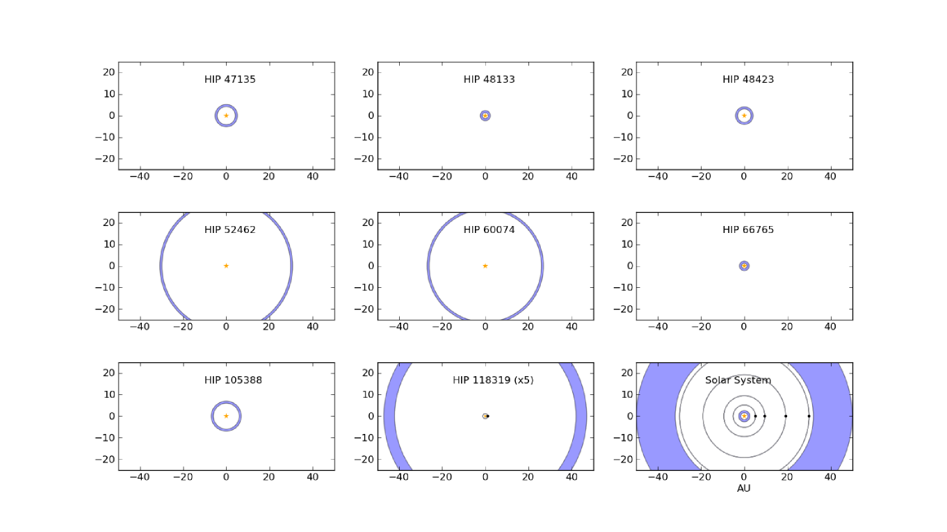
Figure 8: Same as Figure 6. The scale of the debris disk and planet orbit for HIP 118319 is multiplied by 5 for easier visualization.

A histogram of dust radii for those systems with several mid-IR observations is shown in Figure 5. Figures 6, 7, and 8 show a visualization of the dust radii compared with the Solar System’s Kuiper and Asteroid Belts. The mass of the dust can be derived given certain assumptions about the observed dust:

$$M_{dust}=\frac{F_{\nu}d^{2}}{\kappa_{\nu}B_{\nu}(T_{d})}$$ (6)

where d is the distance from Earth and $\kappa$ is the dust opacity, and (in the literature)is often assumed to be 1.7 cm²g^-1 at 800 $\mu$m (Zuckerman & Becklin 1993). At shorter wavelengths, the opacity rises to $\sim$5 cm²g^-1 for a 200 K body (Pollack et al. 1994). The opacity curves from Pollack et al. (1994) employ assumptions about grain size and composition of the dust. However Rhee et al. (2007) provides a relation between the dust mass and the fractional IR luminosity $\tau$ (=L_IR/L_bol):

$$\frac{\tau}{M_{dust}}\propto\frac{1}{\rho aR_{dust}^{2}}$$ (7)

where a is the characteristic radius of the grains. This formula was confirmed empirically using stars with dust masses measured directly from the submillimeter flux, assuming that the dust is in an optically thin ring and that the radius and density of the grains do not change significantly from star to star (see their Figure 4). We similarly calculate dust masses for those stars in our sample with well defined values of $\tau$ (those stars whose IR excess could be fit with a unique blackbody curve). These masses are listed in Table 3.

We expect the amount of dust (parameterized by the fractional infrared luminosity) to decline as a function of stellar age. Over time, there should be more collisions between planetestimals, leading to more debris being ground down to the blow-out size and ejected from the system by radiative forces. This decline in $\tau$ with age has been seen in A stars and solar-type stars (e.g. Su et al. 2006, Bryden et al. 2006, Rhee et al. 2007). We are able to reproduce this trend with our data; the dustiest debris disks are found around young stars ($<$2 Gyr).

5 Stellar Characteristics

5.1 Spectral Type

A summary of our findings broken down by spectral type can be found in Table 4. We find that debris disks were detected predominantly around K-type stars with $\sim$2.5$\sigma$ significance. This seems like a strange result. Since a typical WISE sensitivity limit is 6mJy, a detectable excess would have to be at least 6mJy above the photosphere. For stars at the same distance from Earth, this excess would constitute a higher percentage of the photosphere (a higher $\tau$) for a dim K star than for a bright F star. In other words, a higher $\tau$ would be required to constitute a significant excess around a dim K star, while a lower $\tau$ would be necessary to be detectable at that same level around an F-type star. Thus we are sensitive to smaller $\tau$ in F stars than in K stars. Since our sensitivity is set by the flux of the photosphere at 22 $\mu$m (for a given distance), we should be able to quantify our sensitivity bias. The flux of the photosphere is defined by:

$$F_{\nu}=\pi B_{\nu}(\frac{R}{d})^{2}$$ (8)

where R is the radius of the star and d is the distance to Earth. Since our distance distribution shows no strong dependence on spectral type, we can assume that our F stars and K stars are essentially at the same distance. We also assume that all stars in Table 1 have reached the Rayleigh Jeans tail by 22 $\mu$m so that B_ν$\propto$T. Thus:

$$\frac{F_{\nu,F}}{F_{\nu,K}}=\frac{T_{F}}{T_{K}}(\frac{R_{F}}{R_{K}})^{2}$$ (9)

Using average values for our F and K stars (R_F=1.05R_☉, R_K=0.84R_☉, T_F=6600K, T_K=4100K), we find that F_ν,F/F_ν,K = 2.5. Thus we are 2.5 times more sensitive to F stars than to K stars; Any discrepancy in the detection rate between F stars and K stars would only be magnified when this sensitivity is taken into account. Trilling et al. (2008) also found that K stars had a higher debris disk detection rate than G stars (albeit with a smaller sample size).

5.2 Distance from Earth

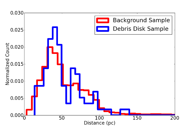
Figure 9: The distribution of debris disks as a function of distance relative to the background sample (which includes the debris disk stars). It is clear that the frequency of debris disk detection has no dependence on distance (inside of 150 pc). Detected debris disks are too few to tell if there is any dependence on distance past 150 pc.

If young stars are preferentially found closer to Earth, then we would be more sensitive to younger stars, and thus our sample would be biased. We examine this possibility in Figure 9. In Figure 9, we can see that there is no obvious correlation between distance and age. Thus we do not believe that a parallax effect is biasing our data.

5.3 Metallicity

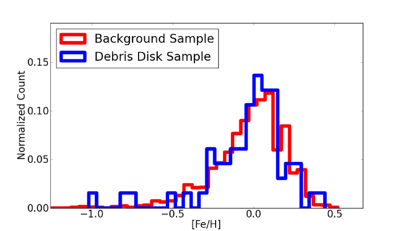
Figure 10: This figure demonstrates the fact that debris disk incidence is not dependent on the metallicity of the host star. A similar trend was noticed by Greaves et al. (2005). This histogram includes 2,110 stars with measured metallicities from Anderson et al. (2012), 66 of which are debris disk hosts.

Since debris disks are found around the dustiest stars, it might be expected that they would also be preferentially found around stars with high metallicities. We gathered metallicity data for as many stars in our sample of 2,820 as possible ($\sim$2,000 stars) from Anderson et al. (2012), and examined the dependence of debris disk incidence on metallicity; no correlation is apparent (Figure 10). This result agrees with the findings of Greaves et al. (2005), who found no correlation between debris disk incidence and metallicity, even when there was a correlation between giant planet incidence and stellar metallicity.

5.4 Planet Hosts

Anderson et al. (2012) provide data on known planet hosts; 136 of our 2,820 stars ($\sim$5$\%$) are known hosts to one or more substellar objects. Four stars out of 98 debris disks presented here ($\sim$4$\%$) are planet hosts, and all have only one known giant planet. This is a surprising result, since we believe that debris disks are signposts of planet formation. The existence of planets, especially giant planets, helps to dynamically stir the population of small bodies to the velocity necessary for a collisional cascade. One therefore might expect to see a high percentage of planet hosts in our debris disk sample. This non-correlation between planet hosts and debris disk hosts was also noted by Bryden et al. (2009).

HIP 3391 is host to a 1.56M_J planet with a semi-major axis of 1.28 AU (Tamuz et al., 2008). HIP 3391 also has a 22 $\mu$m excess, but without additional data points we can only provide an upper limit on the temperature (and a lower limit on the semi major axis of the dust). For a maximum dust temperature of 200 K, the inner semi major axis of the dust is at 2.1 AU. We can thus say that the dust is likely outside the orbit of the planet. We then refitted the dust blackbody, and found a minimum temperature of 45 K, corresponding to a maximum inner semi major axis of the dust of 42 AU.

HIP 7978 is orbited by a 0.9M_J planet at 2.022 AU (Butler et al., 2011)and a 55 K belt of dust 30 AU from the host star (this work). Additional data were taken from the IRS, IRAS and MIPs catalogs and corroborate the IR excess seen by WISE. Thus we are confident about the quoted dust temperature and radius.

HIP 90593 hosts a 0.67M_J planet orbiting 2.24 AU from its host star (Fischer et al. 2009). It also has a single-channel excess indicating a debris disk with temperature 47 K$<$T$<$200 K, corresponding to a range of inner radius 2.62 AU$<$R_dust$<$47.4 AU. The dust is likely located outside of the planet.

HIP 118319 is host to a 0.71M_J which orbits its host star at 0.233 AU (Johnson et al. 2010). It also has a 137 K debris disk (confirmed by a Spitzer 70 $\mu$m data point presented by Bryden et al. 2009) at a minimum radius of 8.43 AU, well outside the orbit of the planet.

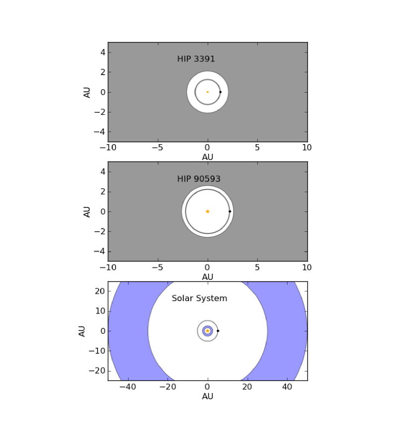
Figure 11: This figure is a visualization of the debris disks around known planet hosts with poorly-determined dust radii. The disks around HIP 3391 and HIP 90593 are located at the minimum possible radius for these systems (corresponding to the maximum possible dust temperature). For comparison, we include the “debris disks” of the solar system (the Asteroid and Kuiper Belts) with the orbit of Jupiter shown.

The results are consistent with a dust location analogous to the Kuiper belt rather than the asteroid belt. Thus our results seem consistent with the physical picture of a debris disk (though we are working with small-number statistics and assuming that there are no undetected close-in planets). A visualization of the debris disks found around planet hosts with ill-determined dust locations can be seen in Figure 11. Note that the dust radii in the top two panels of Figure 11 represent the minimum radii of the dust orbits (or the maximum temperature for the dust blackbody fits).

5.5 Lithium Abundances

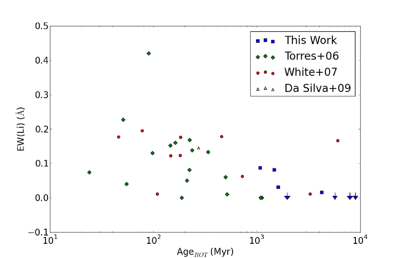
Figure 12: Comparing lithium abundances (measured by the equivalent width (EW) of the Li absorption line at 6707.8 $\AA$) with the ages derived using the activity-rotation-age relation of MH08, we see that there is an apparent decrease in Li as a function of age. We expect the rate of this evolution to be mass-dependent (e.g. Zuckerman & Song 2004); this figure conflates all F, G, and K-type stars.

The abundance of Li absorption at 6707.8 $\AA$ has been cited as a possible tracer of stellar age (e.g. Zuckerman & Song 2004). Twenty-eight stars in our debris disk sample have lithium abundances available in the literature. We were also able to measure lithium abundances for 8 stars in our debris disk sample using the Hamilton Echelle Spectograph on the 3 m Shane Telescope at Lick Observatory. We reached typical sensitivities of 10-15 m$\AA$. The relevant data are listed in Table 5. We compared the Li abundance with the age determined from the activity-rotation-age relation of MH08, and see that the Li abundance decreases as a function of age (see Figure 12). Four of our stars which appear to be old according to their low levels of chromospheric activity also have no detectable lithium. This correlation supports our use of chromospheric activity as an age indicator.

6 ISSUES AND WARNINGS

6.1 Chromospheric Activity Variations

We know that our Sun undergoes variations in magnetic activity over a $\sim$ 11 year period. It is assumed (and in some cases, observed) that other solar-type stars experience similar short-term variations (Duncan et al. 1991). If snapshots of stellar activity are taken, there is no way to tell if the star is being observed during an active period, or a quiet period. Only by taking long ($\sim$10 year) baseline observations can we be certain that we are measuring the average magnetic activity of that star. Few such surveys have been conducted (e.g. Wright et al. 2004), and future surveys will be limited by telescope availability (a spectral resolution of at least 1 $\AA$ is needed to observe the Ca II H & K emission cores which indicate magnetic activity) and the willingness of observers to spend decades on a single sample of stars. This systematic uncertainty introduces an extra source of error in the calculation of age from chromospheric activity. For the Sun, this variation amounts to a 20$\%$ uncertainty in age as calculated from the chromospheric activity during quiescence and during a period of high activity (see Vican 2012 for further discussion of this issue).

6.2 Issues with SED Fitting

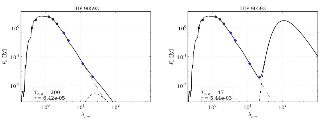
Figure 13: Here we present two possible dust blackbodies which could be fit to the same excess point for HIP 90593 (one of our planet hosts). Clearly there is a large discrepancy in both the temperature and $\tau$ values derived from a single data point excess. Further observations are needed to constrain dust characteristics.

For single band excesses, many different blackbodies could theoretically be fit to the same data point (see Figure 13). The excess we see could be from warm dust emission, or the Wein tail of a blackbody for cooler dust. In some cases, we were able to add data from previous studies (Spitzer, IRAS, etc.) to constrain a blackbody fit to the dust. For those stars for which we found only one data point in excess (i.e. W4), we fit the maximum temperature blackbody, which corresponds to a lower limit to $\tau$ (= L_IR/L_bol). For these stars, it is difficult to say how relevant our calculations for R_dust and M_dust may be, but we include these calculations in Table 1. Follow-up observations with mid-IR instruments such as those on SOFIA might help resolve these discrepancies by providing a second data point with which one could constrain a blackbody dust fit. Physical maps of the dust from ALMA would be the best way to determine the dust radius, since the blackbody radius often underestimates the true radius of the dust (Rodriguez & Zuckerman 2012).

7 CONCLUSIONS AND FUTURE WORK

We examined 2,820 solar type (F, G, and K type) stars using WISE to search for an infrared excess at 22 $\mu$m. We found 98 stars with a clear WISE excess at 22 $\mu$m (a detection rate of 3.5$\%$), 74 of which are presented here for the first time.

An IR excess at 22 $\mu$m is indicative of either hot dust or the Wein tail of a cold dust component. For debris disks with only the 22 $\mu$m data point in excess, follow-up observations are necessary to constrain the properties of the dust. If the dust is truly hot ($\sim$200 K), the drop-off in flux at long wavelengths will make detections with sub-mm instruments (e.g. ALMA, SCUBA-2) unlikely (although a non-detection could also help to constrain the dust temperature; see Bulger et al. 2013). Mid-IR instruments such as FORCAST on SOFIA could be used to confirm the presence of cold dust. It is important to understand the temperature evolution of the dust, especially for those stars which seem to be old ($>$2 Gyr). These old systems are either (1) the tail end of the steady-state evolution of solar type debris disks or (2) the result of cataclysmic collisions between two large rocky bodies (e.g. BD +20 307, Song et al. 2005). Observations in the mid-IR and sub-mm to determine the dust temperature will help distinguish between formation mechanisms.

Partial support for this work was supported by a NASA grant to UCLA and by an NSF Graduate Research Fellowship to Laura Vican. This project made use of the SIMBAD and Two-Micron All Sky Survey (2MASS) databases and VIZIER search engine, operated by CDS in France. The Wide-Field Infrared Survey Explorer is a joint project between the University of California, Los Angeles, and the Jet Propulsion Laboratory, funded by NASA.

We thank Ben Zuckerman for his valuable insight.

Table 1: Chromospheric Activity Targets with IR Excesses

HIP	B-V	SpT	logR′HK	Ref	AgeRHK	AgeROT	Pcalc	Tstar	Rstar	LIR/Lbol	Tdust	Rdust	d	Disk ref
			(dex)		(Myr)	(Myr)	(days)	K	R☉	E-05	K	AU	pc
296	7.60E-01	G8V	-4.5	P13	608	1023	13.32	5700	0.85	5.2	200	1.61	40	none
544	7.50E-01	K0V	-4.384	I10	266	337	7.02	5700	0.82	11.2	200	1.55	14	T08
682	6.30E-01	G2V	-4.359	P13	219	147	3.57	6000	1.03	14.7	100	8.62	40	C09
1365	7.87E-01	G5	-5.029	I10	7144	7931	43.8	5400	3.93	9.6	200	6.66	137	none
1481	5.40E-01	F8	-4.36	P13	221	98	1.98	6200	1.05	9.8	200	2.35	41	Z11
3391	7.30E-01	G5V	-5.021	P13	6994	6855	37.57	5800	1.09	5.9	200	2.13	44	none
5227	8.56E-01	G5V	-4.016	I10	10	24	1.76	5000	4.61	13.1	200	6.70	132	none
5373	8.50E-01	K0V	-4.311	P13	150	211	5.99	5400	0.75	8.4	200	1.27	35	none
5740	6.03E-01	G3V	-5.01	J11	6787	3824	20.96	6000	0.86	8.2	200	1.80	69	none
5881	6.71E-01	G5	-4.8	W04	3202	3051	21.63	5800	0.77	8.7	200	1.51	59	none
6276	7.50E-01	G0	-4.284	I10	120	163	4.65	5600	0.75	7.2	200	1.37	35	Z11
6795	7.80E-01	K0V	-4.507	I10	637	1117	14.34	5500	0.72	12.2	200	1.27	41	none
6856	9.10E-01	K1V	-4.324	P13	166	224	6.52	4900	0.76	12.1	200	1.06	37	Z11*
7576	7.97E-01	G5	-4.41	J11	323	502	9.29	5500	0.77	7.5	200	1.35	24	P09
7978	5.30E-01	F8V	-4.731	P13	2323	1285	7.82	6400	0.99	30.9	55	31.17	17	R07
8867	1.01E+00	G5	-4.654	P13	1556	2568	27.84	4900	0.69	9.4	200	0.96	22	none
8920	5.10E-01	G0	-4.471	I10	499	394	3.03	6100	1.26	400			92	O12
9141	6.60E-01	G3	-4.202	P13	59	78	2.66	5900	0.91	10	145	3.5	42	Z11
10977	9.20E-01	K2	-4.821	P13	3505	4913	37.75	5200	0.73	10.4	200	1.15	31	none
12198	6.20E-01	G5	-4.948	I10	5632	3612	21.28	5900	1.17	7.8	200	2.37	75	none
14684	8.10E-01	G0	-4.4	J11	300	456	8.92	5600	0.77	9.4	140	2.86	40	Z11
14809	7.10E-01	G5	-4.377	I10	252	273	5.9	5900	0.97	6.9	200	1.96	49	Z11
17439	8.80E-01	K1V	-4.496	P13	590	1121	15.85	5300	0.77	19.4	45	24.83	16	none
17903	8.17E-01	G8V	-4.41	J11	323	514	9.62	5600	0.82	8.6	200	1.49	46	none
18828	0.86	K0V	-4.67	I10	1697	2863	26.47	5400	0.7	9.7	200	1.19	43	none
19793	0.657	G3V	-4.432	I10	379	412	6.78	5900	1.04	11	195	2.21	46	none
20737	0.85	K0V	-4.285	P13	121	188	5.62	5400	0.77	20.1	200	1.31	39	none
21091	0.665	G0	-4.43	I10	374	419	6.96	6000	0.94	11.4	200	1.97	67	none
22320	0.82	G8	-5.042	P13	7378	8509	47.19	5600	0.89	7.4	200	1.62	55	none
22787	0.79	K0V	-4.72	P13	2200	3275	26.64	5600	0.78	6.7	200	1.42	26	C09
23243	0.683	G3	-4.96	J11	5853	5031	29.33	5800	0.94	7.9	200	1.84	70	none
26990	0.59	G0V	-4.233	P13	78	64	1.99	6100	1.08	10	200	2.34	52	none
27134	0.849	G5	-4.09	J11	21	55	2.81	5200	0.91	13	200	1.43	50	none
27429	0.554	G0	-4.758	I10	2645	1471	10.02	6300	1.12	8.1	200	2.58	94	none
29391	0.617	G1V	-4.48	J11	531	506	6.95	6100	1.01	7.3	200	2.18	73	none
29442	0.836	K0V	-5.06	J11	7722	8982	49.43	5500	1.05	10.1	200	1.85	76	none
29754	0.618	G2	-5.02	J11	6975	4247	23.21	6000	1.3	8.8	200	2.72	99	none
30030	0.587	G0	-4.177	I10	47	46	1.63	6100	1.05	5.1	200	2.27	50	Z11
33690	0.806	K0IV-V	-4.498	P13	598	1087	14.52	5600	0.82	20.6	94	6.77	18	R07
34147	0.705	G3V	-5.07	J11	7905	7051	36.8	6000	1.17	9	200	2.45	92	none
36129	0.845	G5	-5.003	I10	6656	7943	46.5	5500	0.81	9.7	200	1.42	41	none
36312	0.54	F7V	-4.46	J11	463	301	3.74	6300	1.11	13.9	200	2.56	90	none
36515	0.639	G3V	-4.385	P13	267	223	4.61	5900	0.91	4	200	1.84	22	P09
36948	0.74	G3	-4.317	P13	157	183	4.9	5700	0.8	271	64	14.75	35	R07
38072	0.628	G2V	-4.51	J11	650	665	8.34	5900	0.98	13.8	200	1.98	81	none
41351	0.851	G5	-4.59	J11	1077	1968	21.24	5300	0.7	10.2	200	1.14	43	none
43371	0.772	G5	-4.47	J11	496	839	12.08	5700	0.89	37.6	200	1.68	66	none
44279	0.77	G8IV	-4.91	J11	4951	5745	35.79	5700	1	15.2	200	1.89	65	none
45621	0.869	K0	-4.45	W04	431	782	12.81	5400	1.09	7.8	200	1.85	33	none
45749	0.83	K0V	-4.755	P13	2608	3892	30.62	5300	0.84	10.3	200	1.37	35	none
45950	0.581	G0	-4.544	I10	810	639	7.07	6200	1.15	6.7	200	2.57	71	none
47135	0.588	G2V	-4.34	J11	189	103	2.59	6100	1.09	7	150	4.19	63	S06
47990	0.663	K0	-4.64	J11	1439	1609	14.83	5900	1.15	10	200	2.33	66	none
48133	0.894	K1V	-4.91	J11	4951	6368	42.83	5200	0.87	10.4	200	1.37	26	none
48423	0.72	G5	-4.468	P13	489	724	10.38	5800	0.89	11.1	150	3.09	32	C09
50701	0.623	G3V	-4.97	J11	6038	3876	22.32	5800	1.06	10.1	200	2.07	67	none
50757	0.649	F7V	-4.669	I10	1688	1708	14.92	6000	7.92	16	200	16.57	283	none
51783	0.713	G5	-5.06	J11	7722	7092	37.37	5700	0.87	9.8	200	1.64	62	none
51884	0.855	K0	-4.47	W04	496	920	13.86	5300	1.02	7	200	1.67	34	none
52462	0.877	K1V	-4.338	P13	186	237	6.56	5300	0.73	96.4	40	29.8	22	R07
52933	0.892	K0	-5.06	J11	7722	9136	52.44	5400	0.85	12.7	200	1.44	52	none
54459	1.09	K0	-5.054	P13	7602	8292	56.64	4600	0.58	13.8	190	0.79	26	none
59259	1.06	K2V	-4.299	P13	135	188	6.53	5100	1.1	15.9	200	1.66	51	none
59315	0.7	G5V	-4.294	P13	130	146	4.08	5800	0.83	7.3	200	1.62	38	none
60074	0.6	G2V	-4.385	P13	268	182	3.71	6000	0.94	107	55	26.01	29	R07
66676	0.588	G0V	-4.78	J11	2929	1868	13.31	6000	1.09	12.6	200	2.28	59	none
66765	0.86	K1V	-4.408	P13	317	515	10.03	5400	0.73	8.7	200	1.24	16	T08
67055	0.876	K1V	-4.56	J11	896	1686	19.9	5400	0.72	13.1	200	1.22	45	none
69129	0.875	G5	-4.99	J11	6412	7784	47.22	5300	0.83	10.5	200	1.36	45	none
71640	0.652	G3V	-4.71	J11	2092	2042	16.61	6000	1.05	7.1	200	2.20	72	none
73061	0.783	G8V	-4.98	J11	6224	7027	40.71	5500	2.01	6.22	200	3.53	91	none
73869	0.75	G5	-4.948	P13	5632	6068	36.01	5700	0.91	4.6?	200	1.72	44	H08
75266	1	K3V	-5.014	P13	6853	7913	52.29	5100	0.77	10.1	200	1.16	25	none
76280	0.669	G5	-4.904	P13	4846	4102	25.48	5800	1	9.1	200	1.96	41	none
76704	0.771	G5	-4.578	I10	1001	1684	17.9	5600	2.71	8.9	200	4.94	113	none
76757	0.605	G5	-4.617	I10	1262	1075	10.28	6100	1.08	8.1	200	2.34	73	none
77199	0.97	K2V	-4.155	P13	38	90	4.08	4600	1.03	16.5	200	1.27	41	none
77603	0.7	G2IV/V	-5.059	P13	7703	6762	35.66	5900	2.46	7.1	200	4.98	107	none
78466	0.63	G3V	-4.874	P13	4337	3126	20.11	5800	1.11	9.3	200	2.17	46	none
80129	0.795	G6IV	-5	J11	6599	7509	42.84	5600	2.01	7.9	200	3.66	92	none
87091	0.99	K2IV/V	-4.548	P13	831	1521	20.44	5000	0.68	13.8	200	0.99	31	none
87116	0.71	G6	-4.935	P13	5396	5225	31.3	5700	0.94	8.5	200	1.78	27	none
90593	0.68	G5	-5.017	P13	6919	5694	31.29	6000	1.25	6.4	200	2.62	65	none
92304	0.737	G8V	-4.45	J11	431	655	10.05	5700	1.15	9.34	200	2.17	76	none
96635	0.872	G8IV	-4.18	J11	48	109	4.2	5200	0.67	12.3	200	1.05	35	none
96854	0.7	G6IV/V	-4.961	P13	5862	5380	31.33	5800	0.99	7.1	200	1.94	42	none
98621	0.68	G5V	-4.923	P13	5172	4517	27.45	5800	0.84	7.3	200	1.64	38	none
100942	0.68	G2	-4.947	P13	5614	4810	28.44	6000	1.01	7.8	200	2.11	83	none
101726	0.66	G3V	-4.452	P13	436	499	7.61	5900	0.82	7.1	200	1.66	37	none
105388	0.65	G5V	-4.144	P13	35	51	2.06	5700	0.79	24.3	100	5.97	46	Z11
107457	0.727	G5	-4.46	I10	463	693	10.23	5900	0.87	8.6	200	1.76	38	none
113010	0.875	K1	-4.99	J11	6412	7784	47.22	5100	0.81	17.8	200	1.22	47	none
115527	0.71	G5	-4.394	P13	286	338	6.65	5800	0.84	7.2	200	1.64	30	none
116376	0.702	G5V	-4.57	J11	953	1333	14.28	5700	0.96	8.1	200	1.81	71	none
117247	0.882	K1V	-4.9	J11	4777	6199	41.76	5200	0.77	9.33	200	1.21	36	none
117481	0.5	F6	-4.413	P13	330	375	2.05	6300	1.05	5.9	200	2.42	36	none
117702	0.794	K1V	-5.07	J11	7905	8775	46.73	5300	0.79	11.7	200	1.29	48	none
118319	0.639	G2V	-5.082	I10	8123	5435	28.09	6000	1.89	7.8	137	8.43	94	B09

Note. — P13=Pace 2013, J11=Jenkins et al. 2011, I10=Isaacson & Fischer 2010, W04=Wright et al. 2004, Z11=Zuckerman et al. 2011, B09=Bryden et al. 2009, H08=Hillenbrand et al. 2008, T08=Trilling et al. 2008, Rhee et al. 2007, C09=Carpenter et al. 2009, Plavchan et al. 2009. ^aThese stars have only one data point in excess. Thus, the dust blackbody was fit for the highest possible temperature (and consequently the lowest possible tau).
*Zuckerman et al. 2011 did not find this star to have an IR excess.
Age_RHK is the age calculated directly from the chromospheric activity, while Age_ROT is the age calculated from the rotation period (P_calc), which is in turn
calculated from the chromospheric activity. T_star and R_star come from the Hauschildt et al. 1999 photosphere fits to the optical data points. L_IR/L_bol, T_dust
and R_dust come from the blackbody fit to the mid-IR data points. M_dust is calculated for those stars with a well-determined blackbody fits using the relation
from Rhee et al 2007. The distance from Earth (d) is calculated from the published Hipparcos parallaxes.

Table 2: WISE Data for Stars with Excesses

(1)	(2)	(3)	(4)	(5)	(6)	(7)	(8)	(9)	(10)	(11)	(12)	(13)
HIP	Star Ref	W1phot	W1	W2phot	W2	W3phot	W3	W4phot	W4	W4Err	W4 Ex	SNR
		mJy	mJy	mJy	mJy	mJy	mJy	mJy	mJy	mJy	mJy	mJy
296	P13	721.26	778.2	344.04	414.71	66.42	65.9	18.04	21.45	0.47	3.41	7.22
544	I10	5367.38	6156.72	2560.27	3457.17	494.26	499.93	134.28	184.78	1.7	50.49	29.7
682	P13	1110.77	1158.48	557.44	651.24	100.74	98.25	27.53	41.25	0.71	13.72	19.35
1365	I10	874.3	929.58	398.68	524.49	80.05	82.41	21.68	27.41	0.53	5.73	10.89
1481	P13	1040.67	1072.23	558.27	618.5	97.78	95.35	27.92	41.35	0.51	13.43	26.19
3391	P13	934.35	1009.92	450.45	543.18	85.82	83.89	23.33	28.07	0.48	4.74	9.81
5227	I10	2146.64	2423.89	958.58	1359.92	198.75	215.31	53.69	71.09	0.8	17.4	21.86
5373	P13	644.48	730.95	293.89	376.83	59.01	59.53	15.98	19.77	0.46	3.78	8.24
5740	J11	213.23	219.33	107.01	117.31	19.34	18.82	5.29	7.1	0.36	1.82	5.03
5881	W04	396.03	411.04	190.92	217.64	36.38	35.17	9.89	12.75	0.35	2.86	8.13
6276	I10	701.85	747.29	330.61	397.87	64.75	65.1	17.57	22.61	0.53	5.04	9.6
6795	I10	388.81	529.53	179.32	250.12	35.68	38.73	9.62	13.56	0.4	3.93	9.81
6856	P13	559.89	603.52	252.23	321.32	52.82	53.22	14.34	17.88	0.42	3.54	8.54
7576	J11	1484.76	1613.99	684.76	870.96	136.26	132.57	36.75	48.37	0.62	11.62	18.77
7978	P13	5290.07	6542.38	2851.54	3847.18	492.71	561.5	141.75	216.41	1.73	74.66	43.13
8867	P13	1182.05	1217.55	532.51	680.8	111.52	107.96	30.27	35.74	0.62	5.48	8.91
8920	I10	276.4	324.11	147.9	208.23	25.99	632.34	7.42	538.11	3.66	530.69	145.04
9141	P13	764.2	851.7	387.29	453.04	71.75	72.29	19.89	28.25	0.46	8.37	18.07
10977	P13	671.34	723.58	300.72	385.25	61.57	62.29	16.51	20.39	0.42	3.88	9.32
12198	I10	420.69	437.21	213.2	229.58	39.5	36.84	10.95	14.15	0.39	3.2	8.2
14684	J11	632.44	674.67	297.91	362.86	58.35	58.45	15.83	21.12	0.37	5.29	14.22
14809	I10	503.44	529.53	255.13	286.11	47.27	45.91	13.1	16.82	0.48	3.72	7.79
17439	P13	3193.48	3504.93	1437.64	1871.78	292.39	285.93	78.38	93.74	0.86	15.37	17.83
17903	J11	437.51	485.61	206.09	255.47	40.36	41.38	10.95	13.53	0.42	2.57	6.1
18828	I10	393	432.4	179.21	223.94	35.98	36.67	9.75	12.51	0.37	2.76	7.56
19793	I10	748.66	763.29	379.41	422.03	70.29	66.17	19.48	27.74	0.56	8.26	14.87
20737	P13	596.66	643.71	272.08	345.26	54.63	56.96	14.8	23.96	0.47	9.17	19.5
21091	I10	396.87	422.95	199.17	223.53	35.99	35.15	9.84	14.54	0.55	4.7	8.6
22320	P13	357.68	391.46	168.48	202.55	33	33.32	8.95	11	0.34	2.04	6.02
22787	P13	1427.91	1627.4	672.62	880.44	131.74	134.51	35.75	43.41	0.63	7.66	12.25
23243	J11	276.97	292.34	133.53	157.81	25.44	25.4	6.91	8.84	0.27	1.92	7.14
26990	P13	606.13	630.21	324.34	347.49	56.98	55.94	16.27	22.89	0.37	6.62	18.09
27134	J11	453.46	514.15	203.13	286.91	41.59	47.47	11.15	15.38	0.3	4.23	14.33
27429	I10	201.64	207.15	108.45	112.45	18.74	18.2	5.41	7.33	0.35	1.92	5.5
29391	J11	320.66	343.79	171.59	188.17	30.15	29.88	8.61	11.23	0.37	2.62	7.04
29442	J11	277.26	288.33	127.87	151.68	25.44	25.17	6.86	9.25	0.34	2.39	6.94
29754	J11	256.74	266.62	128.85	140.26	23.28	22.49	6.36	8.51	0.39	2.14	5.48
30030	I10	734.69	838.47	393.14	434.65	69.07	69.33	19.72	24.39	0.54	4.67	8.7
33690	P13	2994.1	3254.83	1410.38	1787.97	276.23	276.16	74.96	110.46	1.11	35.49	32.12
34147	J11	259.54	269.58	130.25	142.87	23.54	23.4	6.43	8.84	0.29	2.41	8.31
36129	I10	611.6	707.76	282.07	366.56	56.13	58.35	15.14	19.22	0.44	4.08	9.32
36312	J11	286.18	304.43	153.91	165.1	26.6	27.27	7.67	12.79	0.33	5.12	15.36
36515	P13	2686.2	3042.82	1361.33	1607.05	252.19	247.21	69.9	86.75	0.94	16.85	17.98
36948	P13	769.41	819.39	367.01	453.04	70.85	73.07	19.25	43.92	0.67	24.67	36.93
38072	J11	258.83	272.83	131.17	144.86	24.3	24.16	6.74	10.57	0.3	3.83	12.94
41351	J11	408.76	443.29	184.01	229.79	37.43	37.21	10.03	12.53	0.46	2.5	5.42
43371	J11	229.69	244.28	109.56	130.9	21.15	23.3	5.75	13.72	0.36	7.98	22.03
44279	J11	361.23	402.8	172.31	209.19	33.26	33.06	9.04	11.54	0.3	2.5	8.35
45621	W04	1469.2	1520.46	669.96	906.66	134.52	140.59	36.44	45.03	0.61	8.6	14.05
45749	P13	756.03	833.08	340.35	456.39	69.22	72.76	18.55	23.87	0.37	5.32	14.3
45950	I10	397.23	414.85	213.1	227.48	37.32	35.95	10.66	13.79	0.41	3.14	7.58
47135	J11	410.75	435.6	219.8	234.5	38.62	38.38	11.03	14.29	0.31	3.26	10.38
47990	J11	424.11	446.57	214.93	244.87	39.82	38.5	11.04	14.77	0.37	3.74	10.21
48133	J11	1528.79	1657.61	684.82	966.42	140.21	150.11	37.59	46.91	0.69	9.32	13.43
48423	P13	1126.01	1093.17	542.85	639.35	103.42	99.47	28.11	42.72	0.65	14.61	22.51
50701	J11	434.93	481.6	209.68	259.74	39.95	41.35	10.86	14.46	0.45	3.6	8.1
50757	I10	1253.79	1341.11	629.22	719.44	113.71	115.75	31.08	51.69	0.6	20.61	34.36
51783	J11	260.14	286.21	124.09	150.57	23.96	24.35	6.51	8.85	0.39	2.34	6.07
51884	W04	1241.11	1369.63	558.72	714.36	113.64	112.27	30.46	36.88	0.66	6.41	9.66
52462	P13	1645.64	1740.48	740.83	970.87	150.67	151.17	40.39	49.51	0.61	9.13	14.86
52933	J11	427.67	467.62	195.02	244.42	39.16	39.81	10.61	14.97	0.46	4.36	9.46
54459	P13	553.42	633.12	250.91	320.44	52.62	50.6	14.64	18.49	0.54	3.85	7.12
59259	P13	607.34	730.95	271.41	388.81	55.94	63.84	15.03	21.12	0.47	6.09	13.09
59315	P13	753.36	820.14	363.19	440.7	69.2	70.16	18.81	24.29	0.42	5.48	13.11
60074	P13	1858.5	1929.89	932.69	1091.14	168.55	164.1	46.07	68.9	0.83	22.83	27.61
66676	J11	538.09	639.57	270.04	337.71	48.8	55.15	13.34	21.39	0.72	8.05	11.2
66765	P13	3127.27	3518.11	1426.05	1848.43	286.33	290.51	77.56	103.45	1.04	25.89	25.02
67055	J11	385.85	414.85	175.95	216.84	35.33	34.9	9.57	12.96	0.38	3.39	8.84
69129	J11	393.61	429.62	177.2	224.36	36.04	37.97	9.66	12.48	0.37	2.82	7.73
71640	J11	331.21	346.97	166.22	185.76	30.04	29.08	8.21	10.73	0.42	2.52	6.06
73061	J11	791.61	867.54	365.09	455.55	72.65	72.45	19.59	23.93	0.52	4.34	8.39
73869	P13	788.33	844.67	376.04	442.73	72.59	69.33	19.72	22.92	0.43	3.2	7.42
75266	P13	1151.08	1215.31	514.4	671.34	106.02	105.75	28.49	34.86	0.49	6.37	13.05
76280	P13	842.04	882.85	405.94	485	77.34	75.46	21.02	27.35	0.46	6.33	13.76
76704	I10	804.07	838.47	378.76	452.63	74.18	72.84	20.13	25.63	0.35	5.5	15.76
76757	I10	377.36	400.21	201.93	214.06	35.48	34.15	10.13	13.2	0.29	3.07	10.58
77199	P13	759.08	847.01	344.15	473.96	72.17	77.73	20.09	27.05	0.5	6.96	13.98
77603	P13	784.36	823.93	397.5	446.83	73.64	70.9	20.41	25	0.53	4.58	8.65
78466	P13	869.66	891.84	419.26	500.43	79.88	78.8	21.71	28.46	0.55	6.75	12.36
80129	J11	823.48	936.46	387.9	480.99	75.97	75.92	20.62	26.28	0.57	5.66	9.97
87091	P13	647.02	699.34	288.93	362.19	59.9	59.63	16.18	21.31	0.45	5.13	11.35
87116	P13	1932.13	2015.57	921.64	1107.84	177.92	164.63	48.34	61.75	1.06	13.41	12.63
90593	P13	631.64	667.25	316.99	358.87	57.28	56.22	15.66	19.89	0.44	4.23	9.66
92304	J11	409.81	541.36	195.48	259.02	37.74	40.41	10.25	13.84	0.44	3.58	8.2
96635	J11	492.56	518.91	220.64	286.64	45.17	46.6	12.11	15.99	0.51	3.87	7.67
96854	P13	789.58	878.8	380.66	470.48	72.52	72.86	19.71	24.83	0.56	5.12	9.21
98621	P13	766.64	856.42	369.59	444.77	70.42	69.46	19.14	23.45	0.57	4.31	7.54
100942	P13	305.13	323.81	153.13	171.14	27.67	27.44	7.56	10.09	0.38	2.52	6.66
101726	P13	732.56	823.17	371.25	450.96	68.78	70	19.06	24.16	0.55	5.1	9.25
105388	P13	509.64	576.35	243.1	304.33	46.93	49.31	12.75	19.67	0.43	6.92	15.99
107457	I10	787.7	877.18	399.19	479.67	73.95	75.28	20.5	27.03	0.34	6.53	19.5
113010	J11	445.83	546.37	199.23	281.41	41.06	46.25	11.04	15.69	0.41	4.65	11.24
115527	P13	1200.58	1319.22	578.8	698.77	110.27	108.37	29.97	38.53	0.6	8.56	14.24
116376	J11	308.29	314.98	147.05	168.32	28.39	27.45	7.71	10.16	0.44	2.45	5.58
117247	J11	603.47	647.27	270.32	356.24	55.35	57.39	14.84	17.94	0.49	3.1	6.35
117481	P13	1565.57	1630.4	841.98	893.46	145.49	140.62	41.98	54.76	0.81	12.78	15.78
117702	J11	346.93	374.19	156.18	194.87	31.77	31.94	8.52	11.36	0.38	2.85	7.56
118319	I10	587.43	592.5	294.81	322.51	53.28	51.75	14.56	19.49	0.51	4.93	9.72

Note. — P13=Pace 2013, J11=Jenkins et al. 2011, I10=Isaacson & Fischer 2010, W04=Wright et al. 2004.

Columns 3, 5, 7, and 9 represent the predicted photospheric values at the W1, W2, W3, and W4 wavelengths. Columns 4, 6, 8, and 10 represent the measured fluxes from WISE. Column 11 is the published WISE uncertainty at W4. Column 12 is excess flux above the photosphere at W4 (W4-W4_phot). Column 13 is the signal to noise ratio of the W4 excess (discussed in Section 2).

Table 3: Supplementary Data for Stars with WISE Excesses

HIP	Mdust (MEarth)	Instrument
544	4.38E-04	IRS, MIPS, IRAS
682	3.20E-03	IRS, MIPS, IRAS
1481	5.81E-04	IRS, MIPS, IRAS
6276	2.49E-04	IRS, MIPS, IRAS
7576	2.55E-04	IRS, MIPS, IRAS
7978	2.43E-02	IRS, MIPS, IRAS
9141	8.83E-04	IRS, MIPS
14684	6.78E-04	IRS, MIPS
17439	1.21E-02	IRS, MIPS, IRAS
22787	2.40E-04	IRS, MIPS, IRAS
30030	2.92E-04	IRS, MIPS, IRAS
33690	3.52E-03	IRS, MIPS, IRAS
36515	1.86E-04	IRS, MIPS, IRAS
36948	1.01E-01	IRS, MIPS, IRAS
44279	7.25E-04	IRAS
47135	7.40E-04	IRS, MIPS
48133	3.59E-04	MSX, IRAS
48423	8.65E-04	IRS, MIPS, IRAS
52462	7.24E-02	IRS, MIPS, IRAS
60074	7.02E-02	IRS, MIPS, IRAS
66765	2.72E-04	IRS, MIPS, IRAS
105388	3.66E-03	IRS, MIPS, IRAS
118319	2.27E-02	IRS, MIPS, IRAS

Table 4: Detection Fraction by Spectral Type

Type	Fraction
F Stars	5/433 (1.15$\pm$0.4$\%$)
G Stars	65/1904 (3.4$\pm$0.4$\%$)
K Stars	28/482 (5.8$\pm$1.0$\%$)

Table 5: Lithium Data

HIP	B-V	EW(H$\alpha$)	EW(Li)	Ref
		$\AA$	m$\AA$
682	0.630	2.34	122	W07
1481	0.540		130	T06
5227	0.856		74	T06
5373	0.850		50	T06
6276	0.750		160	T06
6856	0.910		168	T06
9141	0.660	2.52	195	W07
14684	0.810	1.76	178	W07
14809	0.710		145	D09
17439	0.870		0	T06
22787	0.800	2.15	11	W07
27134	0.850	0	40	T06
27429	0.554	2.342	81	this work
29442	0.836	1.598	$<$10	this work
29754	0.618	1.966	16	this work
30030	0.587	2.63	177	W07
33690	0.790		0	T06
36129	0.845	1.495	$<$5	this work
36515	0.640		81	T06
36948	0.740	2.32	176	W07
41351	0.851	1.477	$<$10	this work
47990	0.663	1.912	31	this work
48423	0.720	2.63	62	W07
52462	0.877		138	T06
59259	1.060		0	T06
59315	0.710		152	T06
60074	0.600	2.79	123	W07
66765	0.860		10	T06
73869	0.750	2.14	166	W07
76757	0.605	1.924	87	this work
77199	0.970		420	T06
90593	0.680	1.825	$<$10	this work
96635	0.872	1.6	11	W07
101726	0.650		60	T06
105388	0.720		227	T06
115527	0.710		133	T06

Note. — T06=Torres et al. 2006, W07=White et al. 2007, D09=Da Silva et al. 2009

Figure 4: This figure shows the evolution of debris disks over time. We used 100 Myr bins and fit a logarithmic profile to the decline of the number of debris disks as a function of age. We find that the number of debris disks declines as e^t0/t where t₀$\sim$175 Myr.

References

- Anderson (2012) Anderson, E. & Francis, Ch., 2012, Astronomy Letters, 38, 331.
- Barnes (2003) Barnes, S. A., 2003, ApJ, 586, 464.
- Beighman (2006) Beichman, C. A., et al., 2006, ApJ, 652, 1674.
- Booth (2009) Booth, M., Wyatt, M. C., Morbidelli, A., Moro-Martn, A., Levison, H. F., 2009, MNRAS, 399, 385.
- Bryden (2006) Bryden, G., Beichman, C. A., Trilling, R. D., et al., 2006, ApJ, 636, 1098.
- Bryden (2009) Bryden, G., et al., Beichman, C. A., Carpenter, J. M., et al., 2009, ApJ, 705, 1226.
- Bulger (2013) Bulger, J., Hufford, T., Schneider, A., et al. 2013, ArXiV:1307.4015.
- Butler (2011) Butler, P., Wright, J., Marcy, G., et al., 2011, ApJ, 646, 505.
- Carpenter (2009) Carpenter, J. M., Bouwman, J., Mamajek, E. E., et al. 2009, ApJS, 181, 197.
- Cutri (2003) Cutri, R. M., Skrutskie, M. F., Van Dyk, S., et al., 2003, VizieR On-line Data Catalog, II/246.
- Cutri (2012) Cutri, R. M., et al., 2012, VizieR Online Data Catalog, 2311.
- Da Silva (2009) Da Silva, L., Torres, C. A. O., De La Reza, R., Quast, G. R., Melo, C. H. F., Sterzik, M. F., 2009, A&A, 508, 833.
- Dodson-Robinson (2011) Dodson-Robinson, S., Beichman, C., Carpenter, J., & Bryden G., 2011, AJ, 141, 11.
- Duncan (1991) Duncan, D. K., Vauhan, A. H., Wilson, O. C., et al., 1991, ApJS, 76, 383.
- Fischer (2009) Fischer, D., Marcy, G., Butler, P., et al., 2009, ApJ, 669, 1336.
- Gaspar (2009) Gspr, A., Rieke, G., Su, K., et al., 2009, ApJ, 697, 1578.
- Gorlova (2006) Gorlova, N., Rieke, G., Muzerolle, J., et al., 2006, ApJ, 649, 1028.
- Greaves (2005) Greaves, J. S., Fischer, D. A., Wyatt, M. C., 2005, MNRAS, 366, 283.
- Hauschildt (1999) Hauschildt, P., Allard, F., & Baron, E., 1999, ApJ, 512, 377.
- Helou & Walker (1988) Helou, G., & Walker, D. W., 1988, IRAS Catalogs and Atlases, 7, 1.
- Heng (2010) Heng & Tremaine, 2010, MNRAS, 401, 867.
- Hillenbrand (2008) Hillenbrand, L. A., Carpenter, J. M., Kim, J. S., et al., 2008, ApJ, 677, 630.
- Hog (2000) Hog, E., Fabricius, C., Makarov, V. V., et al., 2000, A&A, 355, 27.
- Isaacson & Fischer (2010) Isaacson, H. & Fischer, D., 2010, ApJ, 725, 875.
- Jenkins (2011) Jenkins, J. S., Murgas, F., Rojo, P., et al., 2011, A&A, 531, 8.
- Johnson (2010) Johnson, J., Marcy, G., Fischer, D., et al., 2010, ApJ, 647, 600.
- Kennedy (2012) Kennedy, G. M., & Wyatt, M. C., 2012, MNRAS, 426, 91.
- Koerner (2010) Koerner, D. W., Kim, S., Trilling, D. E., Larson, H., et al. 2010, ApJ, 710, L26.
- Mamajek & Hillenbrand (2008) Mamajek, E. E., & Hillenbrand, L. A., 2008, ApJ, 687, 1264. (MH08)
- Matthews (2010) Matthews, B. C., Sibthorpe, B., Kennedy, G., et al., A&A, 518, L135.
- Noyes (1984) Noyes, R. W., Weiss, N. O., Vaughan, A. H., 1984, ApJ, 287, 769.
- Olofsson (2012) Olofsson, J., Juhasz, A., Henning, Th., Mutschke, H., Tamanai, A., Moor, A., Abraham, P., 2012, A&A, 542, 90.
- Pace (2013) Pace, G., 2013, A&A, 551, 8.
- Perryman (1997) Perryman, M. A. C., Lindegren, L., Kovalevsky, J., et al., 1997, A&A, 323, 49.
- Phillips (2010) Phillips, N. M., Greaves, J. S., Dent, W. R. F., et al., 2010, MNRAS, 403, 1089.
- Plavchan (2009) Plavchan, P., Werner, M. W., Chen, C. H., Stapelfeldt, K. R., Su, K. Y. L., Stauffer, J. R., Song, I., 2009, ApJ, 698, 1068.
- Pollack (1994) Pollack, J., Hollenbach, D., Beckwith, S., Simonelli, D., Roush, T. Fong, W., 1994, ApJ, 421, 615.
- Rhee (2007) Rhee J., Song, I., Zuckerman, B, & McElwain, M., 2007, ApJ, 660, 1556.
- Rieke (2005) Rieke, G. H., et al., 2005, ApJ, 620, 1010.
- Rodriguez (2012) Rodriguez, D. R., & Zuckerman, B., 2012, ApJ, 745, 127.
- Roeser (2011) Roeser, S., Schilbach, E., Piskunov, A. E., Kharchenko, N. V., Scholz, T.-D., 2011, A&A, 531, 92.
- Skumanich (1972) Skumanich, A., 1972, ApJ, 171, 565.
- Song (2005) Song, I., Zuckerman, B., Weinberger, A., Becklin, E., 2005, Nature, 436, 363.
- Spangler (2001) Spangler, C., Sargent, A. I., Silverstone, M. D., Becklin, E. E., & Zuckerman, B., 2001, ApJ, 555, 932.
- Su (2006) Su, K., Rieke, G., Stansberry, J., et al., 2006, ApJ, 653, 675.
- Tamuz (2008) Tamuz, O., Segransan, D., Udry, S., et al., 2008, A&A, 480, 33.
- Torres (2006) Torres, C. A. O., Quast, G. R., da Silva, L., De La Reza, R., Melo, C. H. F., Sterzik, M., 2006, A&A, 460, 695.
- Trilling (2008) Trilling, D. E., Bryden, G., Beichman, C. A., et al., 2008, ApJ, 674, 1086.
- Vaughan (1980) Vaughan, A. H. & Preston, G. W., 1980, PASP, 92, 385.
- Vican (2012) Vican, L., 2012, AJ, 143, 135.
- White (2007) White, R. J., Gabor, J. M., Hillenbrand, L. A., 2007, AJ, 133, 2542.
- Wright (2010) Wright, E., Eisenhardt, P., Mainzer, A., et al., 2010, AJ, 140, 1868.
- Wright (2004) Wright, J. T., Marcy, G. W., Butler, R. P., Vogt, S. S., 2004, ApJS, 152, 261.
- Wyatt (2008) Wyatt, M. C., 2008, ARA&A, 46, 339.
- Zuckerman (1993) Zuckerman, B. & Becklin, E. E., 1993, ApJ, 414, 793.
- Zuckerman (2001) Zuckerman, B., 2001, ARA&A, 39, 549.
- Zuckerman (2004) Zuckerman, B. & Song, I., 2004, ARA&A, 42, 685.
- Zuckerman (2011) Zuckerman, B., Rhee, J., Song, I., Bessell, M., 2011, ApJ, 732, 61.